Optical study of superconducting Pr2CuOx with
Abstract
Superconducting Pr2CuOx, (PCO) films with structure and a of 27 K have been investigated by various optical methods in a wide frequency (7 – 55000 cm-1) and temperature (2 to 300 K) range. The optical spectra do not reveal any indication of a normal-state gap formation. A Drude-like peak centered at zero frequency dominates the optical conductivity below 150 K. At higher temperatures, it shifts to finite frequencies. The detailed analysis of the low-frequency conductivity reveals that the Drude peak and a far-infrared (FIR) peak centered at about 300 cm-1persist at all temperatures. The FIR-peak spectral weight is found to grow at the expense of the Drude spectral weight with increasing temperature. The temperature dependence of the penetration depth follows a behavior typical for -wave superconductors. The absolute value of the penetration depth for zero temperature is 1.6 m, indicating a rather low density of the superconducting condensate.
pacs
74.25.Gz, 74.25.nd, 74.72.EkI Introduction
It is commonly accepted that the parent compounds of the superconducting high- cuprates are antiferromagnetic charge-transfer insulators and that superconductivity emerges upon doping either with holes or electrons.[1, 2] There are some similarities but also differences between hole- and electron-doped cuprates. One similarity is that all cuprate superconductors have a perovskite structure with the common feature of square planar copper-oxygen planes separated by rare-earth oxide (charge-reservoir) layers. On the other hand, they differ in that the hole-doped cuprates have a structure characterized by the presence of apical oxygen above and below the CuO2 planes, while the electron-doped cuprates have a structure, where two sites are occupied by oxygen: O(1) in the CuO2 planes and O(2) within the rare-earth oxide layers, with no apical oxygen located directly above the copper in the CuO2 plane, as shown in the inset of Fig. 1. This implies that the structure has six oxygen atoms, two of which are in the apical positions, surrounding each copper (octahedrally coordinated), while in the structure only four oxygens surround each copper (square-planar coordinated).
There is also a large difference between the phase diagrams of hole- and electron-doped cuprates. Whereas the antiferromagnetic phase exists only over a small doping range (0 – 4 %) in hole-doped cuprates, it is more robust in electron-doped cuprates and persists to higher doping levels (0 – 11 %). Superconductivity occurs in a doping range that is almost five times narrower for electron-doped cuprates (11 – 17 %) as compared to the hole-doped counterparts (4 – 32 %). While consensus on the phase diagram exists for the hole-doped side, the situation for the electron-doped cuprates is less obvious.
As early as in 1995, Brinkmann et al.[3] demonstrated that the superconductivity window in Pr2-xCexCuO4 single crystals can be extended down to a doping level of 4 % by a special oxygen reduction and annealing technique. Improved deposition and annealing techniques have recently made it possible to produce thin films of electron-doped parent compounds (CuO4, = Pr, Sm, Nd, Eu, and Gd) with structure that, in fact, are metallic and superconducting at low temperatures.[4, 5, 6, 7, 8, 9, 10]
This sharp contradiction to earlier results is explained as being due to the fact that although apical oxygen should not exist in the ideal structure, in practice (especially in bulk samples) it is usually not completely removed.[10] This apical oxygen in the structure acts as a very strong scatterer and pair breaker.[11] In contrast to bulk samples, the large surface-to-volume ratio of thin films along with their tenuity itself is advantageous in achieving the proper structure with no apical oxygen.
The reported superconductivity in undoped cuprates puts a question mark on the applicability of the charge-transfer-insulator picture to electron-doped cuprates.[12] Remarkably, recent calculations on the basis of a newly developed first-principles method show a radical difference between the parent compounds with and structures.[13, 14, 15] The first are found to be charge-transfer insulators, while the latter, e.g., Pr2CuO4, are essentially metallic and their apparent insulating nature may originate from magnetic long-range order (Slater transition) which is competing with the metallic ground state.[16]
One should note, however, that it is still a question whether or not superconductors are truly undoped or are still doped by possible oxygen vacancies in the O layers during the reduction process. Since bulk -CuO4 superconducting samples have not yet been synthesized, direct measurements of the oxygen distribution are not available so far. Nevertheless, neutron diffraction on Nd2-xCexCuO4+y single crystals shows that it is mostly apical oxygen which is removed during reduction.[17, 18] The synthesis of bulk samples of a nominally undoped -(La,Sm)2CuO4,[19, 20] and of heavily underdoped Pr1.3-xLa0.7CexCuO4+δ[21] gives hope that the oxygen stoichiometry might be determined in the near future for this class of superconductors.

In this paper, we do not touch the issue of oxygen stoichiometry; instead we present a comprehensive broadband optical investigation of Pr2CuOx (PCO) films with . As argued above, it is impossible to rule out doping by oxygen vacancies (if this is the case, differs from 4 in our films). However, we will show that our findings can also be consistently understood within the picture, where superconductivity develops in undoped PCO (i.e., ). We demonstrate that the available PCO samples do show a metallic as well as a superconducting optical response. We find that this response can be reconciled with -wave superconductivity and the density of the superconducting condensate is rather low. We do not observe any indication of a normal-state pseudogap. All this supports ideas that the standard charge-transfer-insulator picture might not be applicable to PCO.
II Experiment
PCO films were grown by molecular beam epitaxy (MBE) [8] on a (110)-oriented 0.35 mm thick DyScO3 substrate. The phase purity of these films was confirmed by x-ray diffraction. The films were 100 nm thick with the axis oriented perpendicular to the film’s surface. Direct-current (dc) resistivity was measured from 4 to 300 K by a standard four-probe method.
Near-normal reflectivity from 40 to 55000 cm-1 (5 – 6800 meV) was measured using a combination of two Fourier-transform spectrometers (Bruker IFs113V and Bruker IFS66V/s) covering frequencies from 40 to 22000 cm-1 and a grating spectrometer for room-temperature reflectivity measurements from 8000 to 55000 cm-1. In order to obtain the absolute reflectivity of the sample, we used an in situ gold (for the infrared) or silver (for the visible) overfilling technique.[22] With this technique, we achieved an absolute accuracy in the reflectivity better than 3 % and the relative error between different temperatures was of the order of 0.5 %. The room temperature reflectivity in the ultraviolet was measured against an aluminum mirror and then corrected for the absolute reflectivity of aluminum.
Normal-incident phase-sensitive transmission at 210 and 250 GHz (7 and 8.3 cm-1) was measured as a function of temperature with a spectrometer employing backward-wave oscillators (BWOs) as sources of coherent radiation.[23] A Mach-Zehnder interferometer arrangement of the spectrometer allows measurements of both the intensity and the phase shift of the wave transmitted through the sample. Using the Fresnel optical formulas for the complex transmission coefficient of the two-layer system, the film’s complex conductivity as well as the penetration depth were directly obtained from these measurements. This experimental method has been previously applied to a large number of different superconductors.[24] Technical details of our experimental procedure can be found in Ref. 25.
Optical properties of bare substrates were obtained from measurements performed in the same frequency and temperature windows as for the thin-film samples.
We investigated two thin films of PCO. The results, obtained on the films, do not demonstrate any significant difference. Hereafter we present results for one of the two films.
III Resistivity
Figure 1 shows the temperature dependence of the resistivity of the PCO film. The resistivity decreases monotonically with decreasing temperature down to 27 K. The width of the superconducting transition is 0.8 K. The temperature dependence of the resistivity can be described by the power law
| (1) |
with = 0.151 mcm, mcmK-n, and from up to 150 K. The quadratic temperature dependence is in agreement with earlier reports on superconducting Nd2-xCexCuO4 films and single crystals for temperatures below 200 K.[26, 27] But, unlike Nd2-xCexCuO4, where a slightly reduced power law with ranging from 1.5 to 1.7 is observed above 200 K, we find a linear temperature dependence in PCO above 210 K. A quadratic temperature dependence is often taken as evidence for Fermi-liquid behavior.[28, 29]
IV Optical properties
IV.1 Raw experimental data

Figure 2 shows the as-measured in-plane (-plane) reflectivity of the PCO film on a DyScO3 substrate versus frequency at various temperatures. At low frequencies, the reflectivity is quite high and increases with decreasing temperature, typical for metals. A number of phonon modes from the substrate and the film appears at frequencies below 700 cm-1. The maxima seen above some 10000 cm-1 can be attributed to interband transitions.

The changes to the reflectivity spectra induced by the superconducting transition are not very well pronounced within our experimental accuracy. This is because of a relatively high transparency of the film. Thus, the results, obtained from the reflectivity measurements, are only discussed in the normal state in the course of the article.
The formation of the superconducting condensate can instead be directly seen by use of our low-frequency phase-sensitive transmission measurements. In Fig. 3 we present examples of these measurements. The onset of the transition into the superconducting state reveals itself immediately as a reduction of the temperature-dependent power transmission and the phase shift.[30] The penetration depth and the superfluid density, obtained from these measurements, are discussed in Sec. IV.6.
IV.2 Normal-state optical conductivity
By applying a thin-film fitting procedure, described in detail in App. A, we extract the film’s complex optical conductivity, , from our reflectivity spectra. Neither BWO data nor values of the dc conductivity in the normal state have been utilized within this fitting procedure.
The real part of the PCO optical conductivity obtained by this modeling is shown in Fig. 4 for various temperatures indicated in the legend. As the lowest frequency of the reflectivity measurements was 40 cm-1 the data obtained from this analysis below this threshold frequency are to be considered as extrapolations and, thus, are shown as dashed lines. Nevertheless, the zero-frequency limit of evolves in accordance with at all temperatures in the normal state (bold points on the vertical left-hand axis of Fig. 4).

At all temperatures above , the optical conductivity of PCO can be disentangled into a Drude component and a set of Lorentz oscillators, representing a broad far-infrared (FIR) band, narrow FIR peaks, a mid-infrared (MIR) band, and interband-transition bands at the highest frequencies:
| Drude + FIR band + FIR peaks + | (2) | ||||
| MIR band + interband transitions. |
This becomes particularly evident from Fig. 5 where all these contributions are shown for 30 and 300 K. (We used the Drude-Lorentz fitting procedure as described in App. A. The FIR and MIR absorption bands have been modeled with two Lorentzians each and we used three Lorentzians for the interband transitions.)
We attribute the narrow and relatively weak peaks at 130 cm-1, 304 cm-1, 343 cm-1, and 500 cm-1 to infrared-active phonon modes. Their frequency positions agree well with the positions of strong phonon modes reported for nonsuperconducting Pr2CuO4 by Homes et al.[31]
It is worth noting here that in addition to the well pronounced phonons, characteristic to the structure, other modes which are not allowed by the crystal structure in the phase, have been observed by Homes et al.[31] The authors have elaborated on the possible origin of these additional modes but concluded eventually that some impurities and/or contributions from different phases may play a role. This conclusion is perfectly in line with claims made in Refs. 4, 5, 6, 7, 8, 9, 10 that the complete removal of all apical oxygen is extremely challenging and absolutely necessary for superconductivity in undoped cuprates.

The bump at about 300 cm-1 in the spectra can be attributed to electron localization. Such behavior is known for the superconducting cuprates[32] and is typical for so-called bad metals where a certain degree of disorder is inherently present.[33, 34]
Using dynamical mean-field theory (DMFT) and iterated perturbation theory, Mutou and Kontani demonstrated[34] that in a strongly correlated metallic state, realized by a large on-site repulsion energy, the optical conductivity develops a Drude peak centered at at low temperatures and a shift of this peak to finite frequencies above the Ioffe-Regel-limit temperature , although the resistivity increases monotonically even at . A temperature evolution of far-infrared , similar to the one observed here, has been reported for underdoped Nd2-xCexCuO4,[27] underdoped La2-xSrxCuO4,[35] and zinc-doped YBCO [YBa2(Cu1-xZnO8].[36]
The two highest-frequency absorption peaks at around 30000 – 40000 cm-1 (4 – 5 eV) are typical for the cuprates and represent transitions into a band formed mostly by oxygen orbitals (see, e.g., Ref. 14). The band slightly below 20000 cm-1 (e.g. around 1.5 – 2 eV) is very similar to the upper Hubbard band. Such absorption bands have been observed, for example, in optical-conductivity studies of insulating undoped Pr2CuO4[37] and Nd2CuO4.[27] It is important to realize that the presence of such a band does not necessarily require a charge-transfer gap. Moreover, LDA + DMFT calculations[14] demonstrated that such a band may perfectly coexist with a quasiparticle absorption peak (e.g. with a metallic state) in the case of undoped Nd2CuO4 with a perfect structure.
IV.3 Spectral weight
We can trace the temperature evolution of each term in Eq. (2). The mid-infrared band is almost invariant with temperature, while the shape of the lower-frequency spectrum (consisting of the Drude contribution and the FIR band) changes. While at temperatures below 150 K the peak in is centered at (the Drude term dominates), it shifts to finite frequencies at K. This shift is an indication of the breakdown of the simple Drude-metal picture. It suggests a continuous change in the charge transport from the low-temperature coherent (Drude) to high-temperature incoherent regimes.[38]
In Fig. 6, we plot the spectral weight (SW) of the Drude term (panel a), the FIR band (panel b), the sum of the two (panel c), and, for completeness, the MIR band (panel d). (The spectral weight of each term in Eq. (8) is just the squared plasma frequency of the term.) As one can see from Fig. 6, the spectral weights plotted in panels (c) and (d) are temperature independent, only the Drude and the FIR-band spectral weights depend on temperature. It is obvious that the spectral weight of the FIR band grows at the expense of the Drude component with increasing temperature. We suggest that this spectral weight transfer between the Drude and the FIR band is related to the change in the transport properties, namely to the change from the quadratic to the linear temperature dependence of which happens at comparable temperatures (Fig. 1).

A qualitative picture of the spectral weight redistribution with temperature in PCO can be studied by means of the total spectral weight:
| (3) |
It is plotted as a function of the cutoff frequency in the inset on the right-hand panel of Fig. 5. At low frequencies , increases with decreasing temperature, and it increases with for all temperatures, finally developing an upturn around 10000 – 15000 cm-1. This upturn is due to interband transitions. Up to 15000 cm-1, the spectral weight shows a temperature dependence. Only at higher frequencies do the spectral-weight curves merge, implying that above 15000 cm-1 (eV) the spectral weight is conserved as temperature changes. In other correlated-electron materials, the spectral weight is known to be conserved also only at frequency scales of a few eV.[1, 39] Thus, our results indicate the presence of electron correlations in PCO.
In order to estimate the spectral weight and the plasma frequency of the itinerant charge carriers only, we set cm-1, thus cutting off the contribution from the interband transitions. This gives a plasma frequency of 17700 cm-1 (2.19 eV), a value comparable to those for other high- cuprates. [27, 40, 41] Using the relation between the charge-carrier density and the plasma frequency (), is estimated to give cm-3 assuming to be equal to the free-electron mass .
IV.4 Extended-Drude analysis
To get further insight into the physics behind the optical response of Pr2CuO4, we analyze the optical conductivity data in terms of the extended (or generalized) Drude model which is widely used for analysis of the optical properties of correlated electron systems.[42, 43] The complex conductivity in this model is given by
| (4) |
where and are the frequency-dependent mass renormalization factor and the optical scattering rate, respectively. Inverting Eq. (4) gives
| (5) |
The frequency-dependent optical scattering rate, obtained on the basis of Eq. (5) with = 2.19 eV, is displayed in Fig. 7 as a function of frequency for various temperatures listed in the legend. At K, the general trend in is to increase with frequency, but this increase is nonmonotonic. This is due to phonons and the localization mode discussed above. This mode reveals itself as a bump at around 230 cm-1 ( 28 meV) in the optical scattering rate. At K, the scattering rate increases rapidly as . This is because at high temperatures the localization mode dominates the Drude contribution as it was discussed in relation to the spectra.
IV.5 Eliashberg analysis and electron-boson spectral density
The optical scattering rate is according to App. B closely related to the electron-exchange boson interaction spectral density [Eq. (10)] which is at the core of normal and superconducting state Eliashberg theory.[44] This theory can be applied to calculate various normal and superconducting state properties and, consequently, it is of quite some interest to gain knowledge on by inverting . This will allow a more detailed analysis of our experimental results.

It was also demonstrated by Schachinger et al.[45] that any nonzero contribution to at some energy will result in an increase of the optical scattering rate. Consequently the bump observed in the optical scattering rate of PCO (Fig. 7) at around cm-1 (meV) cannot be caused by electron-exchange boson interaction and is, therefore, not part of the conducting-electron background. Nevertheless, we concentrate on the normal-state K data and perform a straightforward inversion using the maximum-entropy procedure outlined in App. B by inverting Eq. (10) together with the kernel Eq. (11). As the temperature and frequency independent impurity scattering rate is not known, this is an iterative process which is performed by slowly increasing until a smooth function with no pronounced spikes in the immediate vicinity of has been found. This resulted in meV (meV) which is quite substantial but in good agreement with what has been reported for the system PCCO.[46] Furthermore, we restricted the frequency range of the inversion to meV because between meV, develops only a moderate increase with energy.
It has to be pointed out, though, that Eq. (11) is only approximate. Therefore, we use the spectrum which resulted from the inversion process to calculate the quasiparticle self-energy using the full normal-state infinite-bandwidth Eliashberg equations. The complex infrared conductivity is then calculated using a Kubo formula[47] and the resulting optical scattering rate is calculated from Eq. (5). A comparison of this result with the data requires some adaptation of the original spectrum in order to achieve the best possible agreement with the data. This final spectrum is presented in the inset of Fig. 7. It shows a double-peak structure which is followed by a deep valley and a hump at higher frequencies. The low-energy peak is at meV and the high-energy peak can be found at meV. Similar double-peak spectra have been reported for PCCO by Schachinger et al.[46] and for La1.83Sr0.17CuO4 (a hole-doped cuprate) by Hwang et al.[48] both with a less pronounced low-energy peak. It is most likely that the bump around meV in the PCO data is responsible for this overpronouncement of the low-energy peak in the PCO spectrum.
We found that the mass renormalization factor, which can be calculated as the first inverse moment of , is .
A comparison of theoretical and experimental data for K is presented in Fig. 7(b). The solid (red) curve represents the data while the dashed (black) curve presents the result of our theoretical calculations on the basis of the spectrum shown in the inset. (Of course, good agreement between theory and data cannot be expected in the energy region around the bump at meV.)
IV.6 Penetration depth and Superfluid density
The temperature dependence of the penetration depth of PCO was obtained experimentally by means of phase-sensitive millimeter-wave measurements.[23] Using the Fresnel optical formulas for the complex transmission coefficient, the in-plane complex conductivity of the film was calculated directly from the measured transmission coefficient and phase shift. The penetration depth was then calculated from by using , where is the vacuum speed of light and is the frequency of the incoming radiation. We found m.
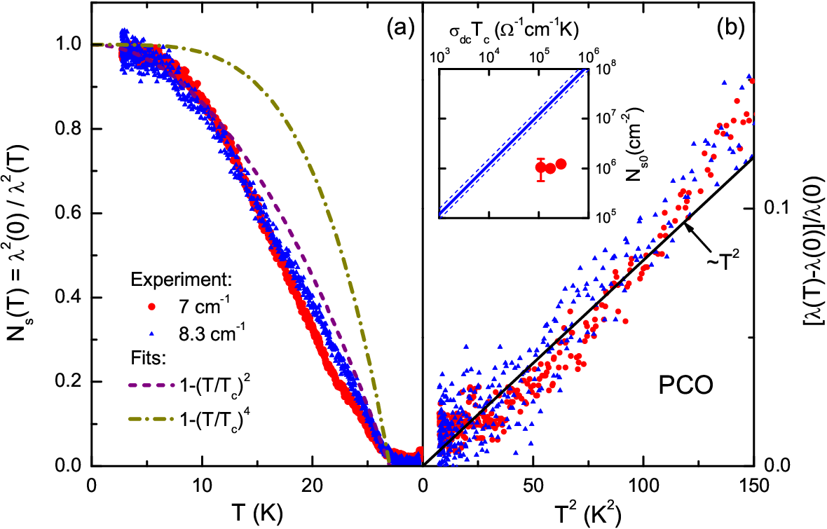
Figure 8(a) presents the normalized superfluid density measured at cm-1 [solid (red) circles] and cm-1 [solid (blue) triangles] vs temperature. We added curves for [thin dashed (purple) curve] and [thin dashed-dotted (olive) curve] for comparison. They are supposed to mimic the temperature dependence of for nodal (-wave) and fully gapped (-wave) superconductivity, respectively. Obviously, the former curve describes the data reasonably well, whereas the fully gapped behavior can certainly be ruled out.
More sensitive is the low-temperature variation of the penetration depth as a function of the square of the temperature. The data are presented in Fig. 8(b) using the same symbols as in Fig. 8(a). For a nodal superconductor a quadratic power law [thin solid (black) line] is to be expected and the data are in agreement with this power law at lowest .
In returning to the absolute value of the zero-temperature penetration depth [] we conclude that the density of the superfluid condensate is very low in PCO as compared to typical values for optimally doped cuprates, where the penetration depth is smaller by a factor of 5 to 10.[49] For example, in optimally doped PCCO nm.[50] This points toward a doping-related nature of superconductivity in our PCO samples, as large values of are typical for either underdoped or overdoped regimes. However, the value of found here is so big, that within this picture our PCO sample must be far off optimal doping. This is rather unlikely, because the critical temperature of our film is definitely too high for a heavily underdoped or overdoped sample. It is also important to note that a possible degradation of while the optical measurements have been performed can be excluded because the dc resistivity measured after the completion of all optical measurements does not differ from the resistivity measured on the fresh film (see bottom panel of Fig. 3).
Furthermore, we would like to note that our second PCO sample had a m and a very similar value of . Another PCO film prepared by a different method (metal organic decomposition vs MBE for the current films) was reported by some of us to have m and K.[51]
It is revealing to note that all these samples do not at all fit a supposedly universal relation reported by Homes et al.[52] which connects the superfluid density [or ] of cuprates to the product of and normal-state conductivity . This relation was obtained from an analysis of experimental data on doped samples, e.g. on doped charge-transfer insulators, and works for all doping levels. According to Zaanen[53] the existence of this universal relation reflects the fact that the normal state of the doped cuprates is extremely viscous (dissipative).[54] All the PCO samples studied here and in Ref. 51 are far off this universal relation (see the inset in Fig. 8). It is tempting to explain this fact as a sign of a possible departure from the charge-transfer-insulator picture in PCO: while Homes’ relation reflects the physics behind the doped-insulator picture, it does not necessarily work any longer whenever this picture loses its validity in cuprates.
Nevertheless, if our samples are indeed doped, it seems to be reasonable to assume that they must be underdoped rather than overdoped. This assumption is based on the method used to prepare the samples (reduction of oxygen content), on the high value of , and on the low superfluid density.
IV.7 Absence of a pseudogap feature
A well-known characteristic feature of the underdoped cuprates is the occurrence of a pseudogap, i.e. a partial normal-state gap in the electronic density of states. Such a pseudogap has been observed in underdoped cuprates by many experimental methods.[55] In optical experiments, the occurrence of a pseudogap below a characteristic temperature can manifest itself in different ways. In hole-doped cuprates, the pseudogap is seen as a suppression of the low-frequency scattering rate. [49] In electron-doped cuprates a suppression of the MIR reflectivity is observed that corresponds to a reduced real-part MIR optical conductivity and to a nonmonotonic behavior of the so-called restricted spectral weight, RSW.[56] Here, RSW is defined as
| (6) |
where , is the restricted frequency range of interest.
It follows from the reflectivity and conductivity data presented in Figs. 2 and 4 that such a normal-state gap is not evident in the current system. The absence of the normal-state pseudogap is further confirmed by the results presented in Fig. 9. In this figure, the restricted spectral weight normalized to the spectral weight at K is plotted as a function of temperature for four frequency ranges as quoted in the legend. It is evident that the normalized restricted spectral weight displays in all four cases a monotonic temperature dependence. This rules out the existence of a normal-state pseudogap.[56] In addition, the optical scattering rate (see Fig. 7) shows (apart from the low-frequency features due to localization, phonon modes, and MIR bands) no temperature-dependent suppression, that might (similarly to the hole-doped cuprates) indicate a pseudo-gap-like feature.[55]

Thus, we conclude that a pseudogap is absent in the PCO films, in contrast to most underdoped high- cuprates. In our view, this difference can be related to the absence of an antiferromagnetic phase in PCO.[10, 12, 57, 21] In electron-doped cuprates, the magnetic order induces the pseudogap. With doping, the Neel temperature decreases monotonically leading to a complete suppression of antiferromagnetic order at higher doping accompanied by the disappearance of the pseudogap. The absence of a pseudogap feature in PCO supports ideas, expressed in Refs. 10, 11, 12, about a strong suppression or even absence of an antiferromagnetic insulating phase in electron-doped cuprates, if the structure (i.e., no apical oxygen) can be managed to survive down to very low or even zero doping levels.
V Conclusions
In our broadband investigation of the optical response of thin PCO films, we unveiled a low-frequency (FIR) collective charge excitation attributed to localization effects. As a function of temperature, the optical spectral weight is redistributed between this mode and the zero-frequency-centered Drude peak: the weight of the FIR mode grows with temperature at the expense of the Drude-peak weight. Such a behavior has been reported in underdoped cuprates and is typical for bad metals.
We found that the optical spectral weight remains temperature-dependent up to 1.9 eV, which indicates strong electron correlations in PCO.
We calculated the electron-boson spectral density and found the mass renormalization factor, at K.
In the millimeter-wave data, we directly observed the formation of the superconducting condensate at . We obtained that the temperature dependence of the London penetration depth at low temperatures follows a quadratic power law. This indicates -wave symmetry which is typical for the cuprates.
Neither the experimental optical data nor their analysis reveal any indication of normal-state gap-like features which could be attributed to the existence of a normal-state pseudogap. This observation is in line with a breakdown of the charge-transfer-insulator picture in PCO.
VI Acknowledgements
We are very grateful to Dr. Hideki Yamamoto for his work on sample preparation and for useful discussions.
Appendix A Thin Films Optical Conductivity
In this work we measured a thin PCO film on top of a DyScO3 substrate. Harbecke[58] studied the optical response of multilayer systems in the most general case, including so-called “coherent” and “incoherent” light propagation.
Coherent propagation is expected when the optical thickness of a medium is comparable or smaller than the wavelength of light. Our measurements span wavelengths from the far-infrared to the ultraviolet. The film thickness is of the order of a few hundred angstroms. We can safely assume coherent propagation throughout the whole measured range. Dealing with the substrate is trickier. Our substrate is 0.5 mm thick. In the far-infrared, light propagates coherently but coherence is gradually lost when moving into the mid-infrared and shorter wavelengths.
To solve this problem, we worked with an unpolished back surface of the substrate. The roughness of our back surface is of the order of 10–50 m, strongly diffusing light of shorter wavelengths. For all that matters, light reflected from the back surface will never reach the detector for this range. A problem might still arise in the far-infrared. However, we have a highly metallic, hence absorbing, film. The contribution from the back surface of the substrate becomes negligible as it implies going twice through the film and being partially diffused by the back surface.
In practice, the effective geometry that best describes our system is a thin film (thickness and complex refraction index ), where light propagates coherently, sitting on top of a half-infinite substrate having a complex refraction index . [59] The near normal incidence reflectivity of such a system is
| (7) |
where , , , and , being the wavelength of light.
In principle, one can perform Kramers-Kronig analysis on the measured reflectivity and numerically invert Eq. 7 to obtain , assuming that we measured the substrate () independently. In practice this procedure is strongly dependent on initial trial values and does not converge with reasonable accuracy. An alternative approach is to model the bulk dielectric function () of the film material. We enter this model into Eq. 7, and utilize a least squares fitting to refine its parameters.
The most straightforward modeling for the dielectric function is the Drude-Lorentz formalism:
| (8) |
In Eq. 8, is the contribution from electronic transitions in the deep-UV. The second term corresponds to a free-carrier Drude response, characterized by a plasma frequency , and a frequency-independent scattering rate . The last term is a sum of Lorentz oscillators; each of them is characterized by a resonance frequency , a line width , and a plasma frequency . All these parameters may freely vary with temperature. This approach has been successfully utilized in several cuprate thin films and a detailed analysis can be found in Santander-Syro et al.[60]
However, the use of Eq. 8 is model dependent. We went a step further in our analysis by adapting the procedure proposed to extract optical functions from single crystal data by Kuzmenko.[61] In his approach the reflectivity is roughly fitted by a Drude-Lorentz dielectric function. A second step is then taken by choosing a variational dielectric function . This function is added to and adjusted in order to describe the total reflectivity within data noise. In Kuzmenko’s paper, is obtained by setting an arbitrary piece-wise imaginary part () of the dielectric function, and calculating the corresponding real part from Kramers-Kronig. This piecewise is obtained by simply setting an arbitrary value at each measured frequency. This value is modified in a least-squares fit so that the reflectivity is properly adjusted. Kuzmenko showed that this method produces optical functions with an accuracy equivalent to Kramers-Kronig.
In principle, Kuzmenko’s method can be straightforwardly adapted to the case of thin films if one replaces the equation for the normal-incidence reflectivity in bulk materials by Eq. 8. However, because of the very large spectral range of our data setting an arbitrary value for at each point measured would be impractical. What we did, instead, was to add a very large number (of the order of 1000) of Lorentz oscillators distributed over the regions where the first fit by the Drude-Lorentz model does not describe properly the data. We fixed the frequency and width of these oscillators and allowed its intensity to vary. In particular, we modified the form shown in Eq. 8 in order to allow for negative values of the numerator. These modified Lorentz oscillators should not be regarded as physical excitations of the systems. They represent a differential correction on the rough Drude-Lorentz dielectric function.
At the end of the procedure, we have a dielectric function
| (9) |
which is a model-independent description of the bulk optical properties of the thin-film material. As a bonus, the rough gives us an overall idea of the physical excitations in the system. However, the obtained dielectric function is model-independent and can be used even when the Drude-Lorentz approach is not expected to work, such as in the superconducting state. Furthermore, usage of the Drude term is not a must even in a metallic state. One could use a large number of Lorentz oscillators instead.
Appendix B Maximum entropy inversion
The optical scattering rate is directly related to the electron-exchange boson interaction spectral density (Eliashberg function) via[62, 45]
| (10) |
The kernel is determined from theory, is an impurity scattering rate and can be calculated by deconvoluting (inverting) Eq. (10). Shulga et al.[63] derived for the normal state the kernel
| (11) | |||||
This kernel is a very good approximation to the exact result of Eliashberg theory. It is valid for any temperature and reduces to the kernel derived by Allen[62] for .
The maximum-entropy method to invert Eq. (10) to gain information on from experimental data was described in detail by Schachinger et al.[64] This process is, of course, an ill-posed problem which does not necessarily allow for an unique solution.
Let us define
| (12) |
where are the experimental data points at discrete energies and is calculated from Eq. (10) and kernel Eq. (11) and is to be regarded as a functional of . Finally, denotes the error bar on the data and is the number of data points. Furthermore, physics requires that the spectral density is positive definite. To achieve this the maximum-entropy method minimizes the functional
| (13) |
with the generalized Shannon-Jones entropy,[65]
| (14) |
which gets maximized in the process. is the constraint function (default model) which reflects a priori knowledge of . In Eq. (13) is a determinative parameter that controls how close the fitting should follow the data while not violating the physical constraints. In our inversion we set for with some small constant indicating that we have no knowledge whatsoever about , thus establishing an unbiased inversion of Eq. (10). Finally we will make use of the historical maximum-entropy method which iterates until the average is achieved with acceptable accuracy.
References
- [1] M. Imada, A. Fujimori, and Y. Tokura, Rev. Mod. Phys. 70, 1039 (1998).
- [2] N. P. Armitage, P. Fournier, and R. L. Greene, Rev. Mod. Phys. 82, 2421 (2010).
- [3] M. Brinkmann, T. Rex, H. Bach, and K. Westerholt, Phys. Rev. Lett. 74, 4927 (1995).
- [4] O. Matsumoto, A. Utsuki, A. Tsukada, H. Yamamoto, T. Manabe, and M. Naito, Phys. Rev. B 79, 100508(R) (2009).
- [5] O. Matsumoto, A. Utsuki, A. Tsukada, H. Yamamoto, T. Manabe, and M. Naito, Physica C 468, 1148 (2008).
- [6] O. Matsumoto, A. Tsukada, H. Yamamoto, T. Manabe, and M. Naito, Physica C 470, 1029 (2010).
- [7] O. Matsumoto, A. Utsuki, A. Tsukada, H. Yamamoto, T. Manabe, and M. Naito, Physica C 469, 924 (2009).
- [8] H. Yamamoto, O. Matsumoto, Y. Krockenberger, K. Yamagami, and M. Naito, Solid State Commun. 151, 771 (2011).
- [9] A. Ikeda, O. Matsumoto, H. Yamamoto, T. Manabe, and M. Naito, Physica C 471, 686 (2011).
- [10] Y. Krockenberger, H. Irie, O. Matsumoto, K. Yamagami, M. Mitsuhashi, A. Tsukada, M. Naito, and H. Yamamoto, Sci. Rep. 3, 2235 (2013).
- [11] T. Sekitani, M. Naito, and N. Miura, Phys. Rev. B 67, 174503 (2003).
- [12] M. Naito, O. Matsumoto, A. Utsuki, A. Tsukada, H. Yamamoto, and T. Manabe, J. Phys.: Conf. Ser. 108, 012037, (2008).
- [13] H. Das and T. Saha-Dasgupta, Phys. Rev. B 79, 134522 (2009).
- [14] C. Weber, K. Haule, and G. Kotliar, Nat. Phys. 6, 574 (2010).
- [15] C. Weber, K. Haule, and G. Kotliar, Phys. Rev. B 82, 125107 (2010).
- [16] Only recently, the first experimental evidence for realization of a Slater transition has been reported: S. Calder, V. O. Garlea, D. F. McMorrow, M. D. Lumsden, M. B. Stone, J. C. Lang, J.-W. Kim, J. A. Schlueter, Y. G. Shi, K. Yamaura, Y. S. Sun, Y. Tsujimoto, and A. D. Christianson, Phys. Rev. Lett. 108, 257209 (2012).
- [17] A. J. Schultz, J. D. Jorgensen, J. L. Peng, and R. L. Greene, Phys. Rev. B 53, 5157 (1996).
- [18] P. G. Radaelli, J. D. Jorgensen, A. J. Schultz, J. L. Peng, and R. L. Greene, Phys. Rev. B 49, 15322 (1994).
- [19] S. Ueda, S. Asai, and M. Naito, Physica C 470, 1173 (2010).
- [20] S. Asai, S. Ueda, M. Naito, Physica C 471, 682 (2011).
- [21] T. Adachi, Y. Mori, A. Takahashi, M. Kato, T. Nishizaki, T. Sasaki, N. Kobayashi, and Y. Koike, J. Phys. Soc. Jpn. 82, 063713 (2013).
- [22] C. C. Homes, M. Reedyk, D. A. Crandles, and T. Timusk, Appl. Opt. 32, 2976 (1993).
- [23] G. V. Kozlov and A. A. Volkov, in Millimeter and Submillimeter Wave Spectroscopy of Solids, edited by G. Grüner (Springer, Berlin, 1998), p. 51.
- [24] M. Dressel, N. Drichko, B. P. Gorshunov, and A. Pimenov, IEEE J. Sel. Top. Quantum Electron. 14, 399 (2008) and references therein.
- [25] T. Fischer, A. V. Pronin, R. Skrotzki, T. Herrmannsdörfer, J. Wosnitza, J. Fiedler, V. Heera, M. Helm, and E. Schachinger, Phys. Rev. B 87, 014502 (2013).
- [26] C. C. Tsuei, A. Gupta, and G. Koren, Physica C 161, 415 (1989).
- [27] Y. Onose, Y. Taguchi, K. Ishizaka, and Y. Tokura, Phys. Rev. B 69, 024504 (2004).
- [28] A. A. Abrikosov, L. P. Gorkov, and I. E. Dzyaloshinski, Methods of Quantum Field Theory in Statistical Physics (Prentice-Hall, Englewood Cliffs, N.J., 1963).
- [29] D. Pines and P. Nozières, The Theory of Quantum Liquids (Addison-Wesley, Reading, 1966), Vol. 1.
- [30] Details of how the superconducting transition and the changes in the temperature-dependent phase-sensitive optical measurements are related, can be found in Ref. 25.
- [31] C. C. Homes, Q. Li, P. Fournier, and R. L. Greene, Phys. Rev. B 66, 144511 (2002).
- [32] D. N. Basov, R. D. Averitt, D. van der Marel, and M. Dressel, Rev. Mod. Phys. 83, 471 (2011).
- [33] V. J. Emery and S. A. Kivelson, Phys. Rev. Lett. 74, 3253 (1995).
- [34] T. Mutou and H. Kontani, Phys. Rev. B 74, 115107 (2006).
- [35] K. Takenaka, R. Shiozaki, S. Okuyama, J. Nohara, A. Osuka, Y. Takayanagi, and S. Sugai, Phys. Rev. B 65, 092405 (2002).
- [36] D. N. Basov, B. Dabrowski, and T. Timusk, Phys. Rev. Lett. 81, 2132 (1998).
- [37] T. Arima, Y. Tokura, and S. Uchida, Phys. Rev. B 48, 6597 (1993).
- [38] A similar effect, although not as a function of temperature, but rather of doping, was reported in: R. P. S. M. Lobo, E. Y. Sherman, D. Racah, Y. Dagan, and N. Bontemps, Phys. Rev. B 65, 104509 (2002).
- [39] M. M. Qazilbash, K. S. Burch, D. Whisler, D. Shrekenhamer, B. G. Chae, H. T. Kim, and D. N. Basov, Phys. Rev. B 74, 205118 (2006).
- [40] S. Uchida, T. Ido, H. Takagi, T. Arima, Y. Tokura, and S. Tajima, Phys. Rev. B 43, 7942 (1991).
- [41] Y. S. Lee, K. Segawa, Z. Q. Li, W. J. Padilla, M. Dumm, S. V. Dordevic, C. C. Homes, Y. Ando, and D. N. Basov, Phys. Rev. B 72, 054529 (2005).
- [42] J. W. Allen and J. C. Mikkelsen, Phys. Rev. B 15, 2952 (1977).
- [43] A. V. Puchkov, D. N. Basov and T. Timusk, J. Phys.: Condens. Matter 8 10049 (1996).
- [44] E. Schachinger and J. P. Carbotte, in: Models and Methods of High- Superconductivity: Some Frontal Aspects, edited by J. K. Srivastava and S. M. Rao, (Nova Science, Hauppauge, NY, 2003), Vol. II, p. 73.
- [45] E. Schachinger, J. J. Tu, and J. P. Carbotte, Phys. Rev. B 67, 214508 (2003).
- [46] E. Schachinger, C. C. Homes, R. P. S. M. Lobo, and J. P. Carbotte, Phys. Rev. B 78, 134522 (2008).
- [47] W. Lee, D. Rainer, and W. Zimmermann, Physica C 159, 535 (1989).
- [48] J. Hwang, E. Schachinger, J. P. Carbotte, F. Gao, D. B. Tanner, and T. Timusk, Phys. Rev. Lett. 100, 137005 (2008).
- [49] D. N. Basov and T. Timusk, Rev. Mod. Phys. 77, 721 (2005).
- [50] A. Zimmers, R. P. S. M. Lobo, N. Bontemps, C. C. Homes, M. C. Barr, Y. Dagan, and R. L. Greene, Phys. Rev. B 70, 132502 (2004).
- [51] A. V. Pronin, T. Fischer, J. Wosnitza, A. Ikeda, and M. Naito, Physica C 473, 11 (2012).
- [52] C. C. Homes, S. V. Dordevic, M. Strongin, D. A. Bonn, R. Liang, W. N. Hardy, S. Komiya, Y. Ando, G. Yu, N. Kaneko, X. Zhao, M. Greven, D. N. Basov, and T. Timusk, Nature 430 539, (2004).
- [53] J. Zaanen, Nature 430, 512 (2004).
- [54] The empirical relation of Ref. 52 also works for conventional superconductors in dirty limit, but because of different reasons, as discussed in Ref. 53.
- [55] T. Timusk and B. Statt, Rep. Prog. Phys. 62, 61 (1999).
- [56] A. Zimmers, J. M. Tomczak, R. P. S. M. Lobo, N. Bontemps, C. P. Hill, M. C. Barr, Y. Dagan, R. L. Greene, A. J. Millis, and C. C. Homes, Europhys. Lett. 70, 225 (2005).
- [57] Y. Krockenberger, H. Yamamoto, A. Tsukada, M. Mitsuhashi, and M. Naito, Phys. Rev. B 85, 184502 (2012).
- [58] B. Harbecke, Appl. Phys. B 39, 165 (1986).
- [59] The validity of considering the substrate as a half-infinite medium was also justified by our measurements of the bare substrate. Multiple reflections within the substrate would reveal themselves either by interference fringes or by a characteristic upturn at frequencies above some 1000 – 2000 cm-1. None of these effects were detected (see the inset of Fig. 2). Instead, the bare-substrate spectra were accurately described by Eq. (7) and a number of Lorentzians.
- [60] A. F. Santander-Syro, R. P. S. M. Lobo, N. Bontemps, W. Lopera, D. Giratá, Z. Konstantinovic, Z. Z. Li, and H. Raffy, Phys. Rev. B 70, 134504 (2004).
- [61] A. B. Kuzmenko, Rev. Sci. Instrum. 76, 083108 (2005).
- [62] P. B. Allen, Phys. Rev. B 3, 305 (1971).
- [63] S. V. Shulga, O. V. Dolgov, and E. G. Maksimov, Physica C 178, 266 (1991).
- [64] E. Schachinger, D. Neuber, and J. P. Carbotte, Phys. Rev. B 73, 184507 (2006).
- [65] See, for example, D. S. Sivia, Data Analysis (Clarendon Press, Oxford, 1996).