h–principle for 4–dimensional Contact Foliations

The central objects in this article are contact foliations. This notion generalizes the concept of a contact fibration and intertwines the contact topology of the leaves with the their global behaviour governed by the foliation.

The manifold $V$ must be even dimensional for a contact foliation $({\mathcal{F}},\xi)$ to exist. Given a codimension–2 distribution $\xi\subset T{\mathcal{F}}$, an extension of $\xi$ is a codimension–1 distribution $\Theta\subset TV$ such that $\xi=\Theta\cap T{\mathcal{F}}$. The reader should compare this with a contact fibration [CP, Le]. A pair $({\mathcal{F}},\Theta)$ such that $\Theta\cap{\mathcal{F}}$ is a contact structure on the leaves will be referred to as an extended contact foliation. A pair $(\beta,\alpha)$ of $1$–forms is associated to $({\mathcal{F}},\Theta)$ if $\ker\beta=T{\mathcal{F}}$ and $\ker\alpha=\Theta$.

The contact connection is a line field contained in $\Theta$ and satisfying $\xi\oplus{\mathcal{H}}_{\Theta}=\Theta$. In particular, $T{\mathcal{F}}\oplus{\mathcal{H}}_{\Theta}=TV$. Observe that $d\alpha$ does not necessarily vanish on ${\mathcal{H}}_{\Theta}$: rather, contraction with a vector field in ${\mathcal{H}}_{\Theta}$ yields a form that vanishes on $\xi$ and ${\mathcal{H}}_{\Theta}$, so it must be a multiple of $\alpha$. Note that the contact connection does not depend on the choice of $\alpha$, it only depends on the extended distribution $\Theta$. Contact connections have been used before in the case of contact fibrations, see for instance [CP].

Given an extension $({\mathcal{F}},\Theta)$ defined by $(\beta,\alpha)$, we associate two vector fields $T$ and $R$ uniquely determined by the following equations:

These vector fields $T$ and $R$ will be referred to as the transverse field and the Reeb field of $(\beta,\alpha)$. Note that ${\mathcal{H}}_{\Theta}=\langle T\rangle$.

The parallel transport between the leaves in Example 7 is by contactomorphisms. This is a particular instance of the following

Consider the space ${\mathcal{E}}({\mathcal{F}},\xi)=\{({\mathcal{F}},\Theta):({\mathcal{F}},\Theta)\mbox{ is an extension of }({\mathcal{F}},\xi)\}$. The space of connection $1$–forms in a smooth vector bundle has a natural affine structure. This is also the case for ${\mathcal{E}}({\mathcal{F}},\xi)$. Indeed, one can prove the following

In particular, the space ${\mathcal{E}}({\mathcal{F}},\xi)$ is contractible and the choice of extension for a foliated contact structure is unique up to homotopy.

The previous definitions and facts suffice for the reader to follow the proof of Theorem 1. However, we consider appropriate to include a short discussion on the transformations appearing in foliated contact topology. A diffeomorphism of $V$ that preserves both ${\mathcal{F}}$ and $\xi$ will be called a foliated contactomorphism. The infinitesimal symmetries are described as follows.

If an extension $({\mathcal{F}},\Theta)$ is fixed and an associated pair $(\beta,\alpha)$ is given, the space of contact vector fields is equivalently defined as:

A flow by foliated contactomorphisms is induced by a 1–parametric family of contact vector fields.

This incursion into foliated contact vector fields and the use of extensions of a contact foliation lead to a proof of the foliated version of Gray’s stability in contact topology (i.e. the moduli space of contact structures is discrete). The precise statement reads as follows.

There are foliated analogues of several concepts and results in contact topology. We have introduced the essential notions, and the reader should be able to define any further objects and prove foliated versions of basic results. See for instance Lemmas 18 and 20.

In the next subsection we shall discuss in brief foliated symplectic topology. There is a subtlety added in comparison to the contact case, yet experts familiar with symplectic and Hamiltonian fibrations will (hopefully) find the definitions quite reasonable.

In this subsection we treat the case of (strong) symplectic foliations. It is not required in order to prove Theorem 1, however it serves as a foundational subsection and contributes to a better understanding of foliated contact topology.

We begin with the simpler notion of a symplectic foliation.

These objects are a generalisation of symplectic fibrations, see [MS], and they are also referred to as regular Poisson foliations, confer [He]. The subtlety in the symplectic case, in contrast to the contact case, is the closedness of the possible extensions of the 2–form $\omega$. Given a symplectic foliation, we can consider the space of closed $2$–forms $\Omega$ such that $\Omega|_{T{\mathcal{F}}}=\omega$. Then, a pair $({\mathcal{F}},\Omega)$ with such an $\Omega$ will be called an extension of $({\mathcal{F}},\omega)$. Symplectic foliations with a fixed extension are also referred to as $2$–calibrated structures [IM2].

The closedness of the extension 2–form is relevant in regard to the concept of a symplectic connection.

If a defining form $\beta$ for the foliation is chosen, a symplectic connection determines a distinguished transverse vector field $T$ defined by

a notion that was already defined, for a particular subclass of symplectic foliations, in [GMP]. The analogue of Lemma 8 for symplectic foliations reads as follows.

Note that closedness of $\Omega$ is exactly the condition one needs to ensure that the parallel transport induced by the symplectic connection is by symplectomorphisms in the particular case of a fibration, see [MS, Lemma 6.18].

Consider the space $\mathfrak{E}({\mathcal{F}},\omega)$ of all extensions of $\omega$. Notice that closedness is a non–trivial condition, and $\mathfrak{E}({\mathcal{F}},\omega)$ might be empty. This differs from the flexibility found in contact foliations (this difference already appears between contact and symplectic fibrations). The symplectic version of Lemma 9 also holds.

In order to distinguish the cases in which an extension exists (and thus there is a parallel transport by symplectomorphisms) we introduce the following notation.

A strong symplectic foliation will be abbreviated to an $s$–symplectic foliation. Observe that the assumption of a foliation being $s$–symplectic is meaningful. Indeed, many results from symplectic topology are likely to extend to this special class of foliations. For instance, approximately holomorphic techniques, see [Ma1].

Let us establish Moser’s Lemma and Darboux’s Theorem for the case of foliated symplectic topology. Their proofs are left to the reader.

Darboux’s Theorem shall provide a local normal form for a symplectic foliation. We describe this local model in the following example.

We can state Darboux’s Theorem in foliated symplectic topology.

The strict version of Darboux’s Theorem also holds.

These Darboux’s Theorems also hold for contact foliations (their proofs rely on the foliated Gray’s stability theorem). The corresponding statements and details are left to the interested reader.

This Section 1 has introduced the basic definitions and properties of contact and symplectic foliations. Section 2 provides some constructions and examples which illustrate the richness of these geometries.

This is a property associated to a codimension one foliation ${\mathcal{F}}$ on a smooth ($n+1$)–fold $V$. A foliation ${\mathcal{F}}$ on a smooth manifold $V$ is said to be (topologically) taut if for every leaf there exists a transverse circle intersecting that leaf.

There is also the notion of a geometrically taut foliation: ${\mathcal{F}}$ is geometrically taut if there exists a closed form $\tau\in\Omega^{n}(V)$ such that $i_{\mathcal{L}}^{*}\tau$ is a volume form for every leaf ${\mathcal{L}}$. This is equivalent to the existence of a complete non–vanishing vector field $X\in\mathfrak{X}(V)$ transverse to ${\mathcal{F}}$ and preserving some volume form $\nu\in\Omega^{n+1}(V)$ (i.e. ${\mathcal{L}}_{X}\nu=0$).

A taut foliation ${\mathcal{F}}$ is geometrically taut, and the converse holds if the ambient manifold $V$ is closed, see [Su, Theorem II.20]. Observe that an $s$–symplectic foliation $(M,{\mathcal{F}},\omega)$ is geometrically taut, since for any choice of extension $\Omega$, we have that the closed $(2n)$–form $\Omega^{n}$ is a leafwise volume form. Thus, the $s$–symplectic foliation ${\mathcal{F}}$ is taut if $M$ is closed. There are however non–taut foliations which support contact structures on closed manifolds. We will construct a family of examples in Subsection 2.3 (and this is also consequence of the Theorem 1).

Theorem 1 is first proven for the case of a taut foliation ${\mathcal{F}}$ in Section 4.

Let us construct a foliated contact structure on a codimension one foliation on the 4–torus ${\mathbb{T}}^{4}$. There are four natural type of foliations on the 4–torus obtained by quotienting the horizontal foliation of a 4–polydisk by 3–polydisks. In coordinates ${\mathbb{T}}^{4}(t,x,y,z)$ their defining equations have the form

The horizontal foliation of ${\mathbb{T}}^{4}$ by 3–tori is given by a tuple $(p,q,r,s)$ of rationally dependent numbers. In case there are two sets of rationally dependent numbers, the leaves are diffeomorphic to ${\mathbb{T}}^{2}\times\mathbb{R}$. If there are three sets of rationally dependent values, the leaves are diffeomorphic to $\mathbb{S}^{1}\times\mathbb{R}^{2}$. Finally, if the numbers are rationally independent the leaves are dense $\mathbb{R}^{3}$ in ${\mathbb{T}}^{4}$.

Let us endow such foliations with a foliated contact structure. Suppose that $s=1$ and consider the form

This is a well–defined 1–form on ${\mathbb{T}}^{4}$. The condition for a foliated contact structure reads

Hence $\alpha$ defines a foliated contact structure for any 1–form $\beta$ as above. In particular, we obtain a contact foliation with (dense) tight contact $\mathbb{R}^{3}$ leaves on ${\mathbb{T}}^{4}$.

This example is of a particular interest regarding a Weinstein–type conjecture in foliated contact topology. In this last irrational case, the foliated Reeb vector field has no periodic orbits (even though the ambient manifold ${\mathbb{T}}^{4}$ is compact). This example must be placed in contrast to the case with overtwisted leaves, see [PP].

Consider a pair $(W,{\mathcal{F}})$ given by a codimension one cooriented foliation ${\mathcal{F}}$ on $W$ and the manifold $V=\mathbb{P}(T^{*}{\mathcal{F}})$, the projectivised cotangent bundle of ${\mathcal{F}}$. There exists a natural projection $\pi:V\longrightarrow W$ and hence the foliation ${\mathcal{F}}$ can be pull–backed to $V$ to a foliation ${\mathcal{F}}_{V}=\pi^{*}{\mathcal{F}}$. The projectivization of the cotangent bundle of a manifold has a canonical contact structure. Similarly, the foliated manifold $V$ has a natural foliated contact structure defined by

where the point $p$ is identified with a $1$–form in $T_{\pi(p)}{\mathcal{F}}$ (which is well–defined up to scaling).

In particular, the foliated contact structure restricted to a leaf coincides with the space of contact elements of the leaf. In the same vein, the sphere bundle $S=\mathbb{S}(T^{*}{\mathcal{F}})$ associated to the cotangent space of the foliation is a foliated contact manifold $(S,{\mathcal{F}}_{S},\xi_{S})$ that restricts to the space of cooriented contact elements over each leaf. The foliated contact structure (${\mathcal{F}}_{S},\xi_{S})$ can also be obtained via the pullback of $({\mathcal{F}}_{V},\xi_{V})$ through the double–cover $S\longrightarrow V$.

Let us provide an example of two non–isotopic foliated contact structure which are homotopic as foliated almost contact structures.

A particular example we consider clarifying is constructed in the following proposition.

Note that the same proof works for any foliation $(M^{3},{\mathcal{F}})$ with a Reeb component: the space of foliated contact elements associated to $(M^{3},{\mathcal{F}})$ possesses a foliated contact structure with tight and overtwisted leaves.

Let $(M,\lambda)$ be an exact symplectic manifold, the contactization $\mathcal{C}(M,\lambda)$ of $(M,\lambda)$ is the manifold $M\times\mathbb{R}(t)$ endowed with the contact structure $\xi=\ker(\lambda-dt)$.

In case the symplectic manifold $(M,\omega)$ is not exact there also exists a contactization (known as prequantization). Let $({\mathcal{F}},\omega)$ be an $s$–symplectic foliation on $M$, with an extension $\Omega$ such that $[\Omega/(2\pi)]$ is integral and consider the principal circle bundle $L_{\Omega}\longrightarrow M$ associated to $\Omega$. Construct a connection 1–form $\alpha\in\Omega^{1}(L_{\Omega})$ with curvature $\Omega$.

Note that the Boothby–Wang contact foliation over a closed base is taut because the $s$–symplectic foliation is taut.

Let $(V,\xi=\ker\alpha)$ a contact manifold. The symplectic manifold $(V\times\mathbb{\mathbb{R}}(t),d(e^{t}\alpha))$ is known as the symplectization of $(V,\xi)$.

Notice that $\Omega=d(e^{t}\alpha)$ is an extension of $\omega$ (and thus $\Omega$ is exact). The $s$–symplectic foliation obtained in the construction does not depend on the particular choice of $\alpha$ and $\Theta$ (up to foliated symplectomorphism).

Observe that the symplectization is geometrically taut, since it is a $s$–symplectic foliation. However it is not necessarily taut, if this were the case the starting contact foliation would be taut.

Consider a contact foliation $(V,{\mathcal{F}},\xi)$ on a ($2n+2$)–fold $V$ and let $(S,{\mathcal{F}}|_{S},\xi|_{S})$ be a foliated contact divisor, i.e. $S$ is a $2n$–dimensional submanifold transverse to ${\mathcal{F}}$ and $\xi$ such that $\xi|_{W}$ is a leafwise contact distribution.

Generalizing [Ge, Theorem 2.5.15], Lemma 12 implies that the tubular neighbourhood of $W$ is uniquely determined by the conformal symplectic structure of its normal bundle. Since its normal bundle is a 2–dimensional disc bundle, the foliated contact structure of its tubular neighbourhood depends only on its oriented topological type.

Let $(\alpha_{S},\beta_{S})$ be an associated pair for $(S,{\mathcal{F}}_{S},\xi_{S})$ and consider its pull–back (still denoted by $(\alpha_{S},\beta_{S})$) to the manifold $S\times D^{2}_{2\varepsilon}(r,\theta)$. Suppose that the normal bundle of $S$ is trivial and thus there exists a neighborhood $\operatorname{Op}(S)$ and an embedding $\phi:S\times D^{2}_{2\varepsilon}\to\operatorname{Op}(S)$ such that the pull–back of the contact foliation is

This is the local model along the foliated contact divisor. We describe the framework in which we can perform a foliated contact connected sum along such a foliated contact divisor.

Let $(V_{0},{\mathcal{F}}_{0},\xi_{0})$ and $(V_{1},{\mathcal{F}}_{1},\xi_{1})$ be two contact foliations and $f_{0}:S\longrightarrow V_{0}$, $f_{1}:S\longrightarrow V_{1}$ two embeddings of $S$ as a foliated contact divisor with trivial normal bundle. There exists two neighbourhoods $\operatorname{Op}(S,V_{0})$ and $\operatorname{Op}(S,V_{1})$ and two embeddings

conforming the local model described above (and extending $f_{0}$ and $f_{1}$).

The gluing region is the open manifold $\mathcal{S}=S\times(-\varepsilon^{2},\varepsilon^{2})\times\mathbb{S}^{1}$ contact foliated as

Note the linearity in the $t$–coordinate. Define the maps

Then the topological connected sum

with the foliated contact models introduced above inherits a foliated contact structure. The related construction for symplectic foliations is discussed in [IM2], though it does not preserve strongness.

Sections 1 and 2 have presented the definitions, results and constructions in foliated contact and symplectic topology. The remaining Sections 3, 4 and 5 shall focus on the proof of Theorem 1.

The h–principles proven by M. Gromov [Gr2] include a parametric (and relative) h–principle for the existence of contact structures on open manifolds. This h–principle can also be proven using the holonomic approximation developed in [EM].

Let us state the exact h–principle we use in the proof of Theorem 1.

Observe that the dependence on the parameter can be supposed to be smooth since the condition for a contact structure is open (and thus preserved by small smoothing perturbations). Theorem 26 allows us to construct a foliated contact structure in a neighborhood of the 3–skeleton, this is explained in Subsection 3.4.

There also exists a subclass of contact closed manifolds satisfying an existence h–principle. This is the main result in [El]. Let us define this class. The disk

with the germ of the contact structure is the standard overtwisted disk. An almost contact 3–fold $(V^{3},\xi)$ is said to be overtwisted if there exists an embedded disk $D$ such that $(\operatorname{Op}(D),\xi)$ is contactomorphic to the standard overtwisted disk. The class of overtwisted (almost) contact manifolds is flexible, i.e. it is classified by its homotopy data. The corresponding h–principle can be stated as follows.

Theorem 27 is used in Sections 4 and 5 in order to extend the foliated contact structure on a neighborhood of the 3–skeleton to the interior of the 4–cells.

Consider a pair $(V^{4},{\mathcal{F}})$. A cell $\sigma:\Delta\longrightarrow V$ is said to be linear with respect to ${\mathcal{F}}$ if its image is contained in the image of a trivializing foliation chart for ${\mathcal{F}}$ and the foliation $\sigma^{*}{\mathcal{F}}$ is transverse to all the facets of $\Delta$.

In a linear cell the height function in the foliation chart yields a function in $\Delta$ with one maximum and one minimum in two vertices and no critical points elsewhere. See Figure 2.

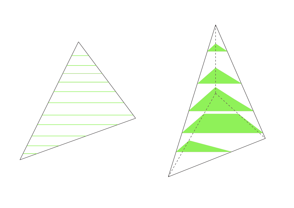
A triangulation ${\mathcal{T}}$ of $V$ is adapted to the foliation ${\mathcal{F}}$ if all its simplices are linear with respect to ${\mathcal{F}}$. This corresponds to a distribution being in general position with respect to a triangulation. There always exists a triangulation on $V$ adapted to ${\mathcal{F}}$, see [Th]. The $i$–skeleton of $V$ with respect to this triangulation ${\mathcal{T}}$ is denoted by $V^{(i)}$.

In order to use Theorems 26 and 27 we require precise local models. The following lemma provides explicit models: these allow us to control the deformations that we obtain by applying the above h–principles (with the suitable parameter spaces $L\subset K$ in each occasion).

Consider the standard 3–ball $D^{3}_{r}\subset\mathbb{R}^{3}$ of radius $r$ and let us fix a sequence of equators $\mathbb{S}^{0}_{r}\subset\mathbb{S}^{1}_{r}\subset\mathbb{S}^{2}_{r}$ respectively bounding flat disks $D^{1}_{r}\subset D^{2}_{r}\subset D^{3}_{r}$. Given the interval $I=[0,1]$, the product foliation $\{\{t\}\times D^{3}_{r}\}_{t\in[0,1]}$ is denoted by ${\mathcal{F}}_{I\times D^{3}_{r}}$. We can state the main lemma of this Subsection:

See Figure 3 for a schematic representation of the statement.

References

- [BEM] M.S. Borman, Y. Eliashberg, E. Murphy, Existence and classification of overtwisted contact structures in all dimensions, arXiv:1404.6157.
- [CP] R. Casals, F. Presas, A remark on the Reeb flow for spheres, to appear in J. Symp. Geom.
- [El] Y. Eliashberg, Classification of overtwisted contact structures on 3–manifolds, Invent. Math. 98 (1989), 623–637.
- [EKP] Y. Eliashberg, S.S. Kim, and L. Polterovich, Geometry of contact transformations and domains: orderability versus squeezing, Geom. Topol. 10 (2006), 1635–1747.
- [EM] Y. Eliashberg, N. Mishachev, Introduction to the h–Principle, Graduate studies in Mathematics, Vol. 48, AMS publications (2002). Geom. Funct. Anal. 10 (2000), 1448–1476.
- [FO] K. Fukaya, K. Ono, Arnold conjecture and Gromov-Witten invariant. Topology 38 (1999), no. 5, 933–1048.
- [Ge] H. Geiges, An Introduction to Contact Topology, Cambr. Studies in Adv. Math. 109, Cambr. Univ. Press 2008.
- [GMP] V. Guillemin, E. Miranda, A.R. Pires, Codimension one symplectic foliations and regular Poisson structures, Bull. Braz. Math. Soc. (N.S.) 42 (2011), no. 4, 607-623.
- [Gr1] M. Gromov, Pseudo holomorphic curves in symplectic manifolds, Invent. Math. 82 (1985) 307–347.
- [Gr2] M. Gromov, Partial Differential Relations, Ergeb. Math. Grenzgeb. 9 (1986), Springer–Verlag.
- [He] G. Hector, Une nouvelle obstruction à l’intégrabilité des variétés de Poisson régulières. Hokkaido Math. J. 21 (1992) No. 1 159–185.
- [HMS] G. Hector, E. Macías, M. Saralegi, Lemme de Moser feuilleté et classification des variétés de Poisson régulières. Publ. Mat. 33 (1989), no. 3, 423–430.
- [IM] A. Ibort, D. Martínez-Torres, A new construction of Poisson manifolds, Journal of Symplectic Geometry 2 (2003), No.1, 83–107.
- [IM2] A. Ibort, D. Martínez-Torres, Approximately holomorphic geometry and estimated transversality on 2-calibrated manifolds. C. R. Math. Acad. Sci. Paris 338 (2004), no. 9, 709–712.
- [Le] E. Lerman, Contact fiber bundles. J. Geom. Phys. 49 (2004), no. 1, 5266.
- [LT] G. Liu, G. Tian, Floer homology and Arnold conjecture, J. Diff. Geom. 49 (1998) 1–74.
- [Lu] R. Lutz, Sur l’existence de certaines formes différentielles remarquables sur la sphère , C.R. Acad. Sci. Paris 270 (1970) 1597–1599.
- [Ma] J. Martinet, Formes de contact sur les variétés de dimension 3. Proc. Liverpool Sing. Symp. II, Lect. Notes in Math. 209 (1971), 142–163.
- [Ma1] D. Martínez Torres, Codimension–one foliations calibrated by nondegenerate closed 2–forms. Pacific J. Math. 261 (2013), no. 1, 165–217.
- [MS] McDuff, Dusa; Salamon, Dietmar, Introduction to symplectic topology. Second edition. Oxford Mathematical Monographs. The Clarendon Press, Oxford University Press, New York, 1998.
- [PP] A. del Pino, F. Presas, Foliated Weinstein conjecture, preprint.
- [Po] L. Polterovich, The geometry of the group of symplectic diffeomorphisms, Lectures in Mathematics ETH Zürich, Birkhäuser (2001).
- [Su] D. Sullivan, Cycles for the dynamical study of foliated manifold and complex manifolds, Invent. Math. 36, 225–255 (1976).
- [Ta] C. H. Taubes, The Seiberg–Witten equations and the Weinstein conjecture. Geom. Topol. 11 (2007) 2117–2202.
- [Th] W.P. Thurston, Existence of codimension–one foliations, Ann. of Math. 104 (1976) 249–268.
- [We] A. Weinstein, Periodic orbits for convex Hamiltonian systems, Ann. of Math. 108 (1978) 507–518.