A Fuzzy Clustering Algorithm for the Mode-Seeking Framework
Abstract
In this paper, we propose a new fuzzy clustering algorithm based on the mode-seeking framework. Given a dataset in , we define regions of high density that we call cluster cores. We then consider a random walk on a neighborhood graph built on top of our data points which is designed to be attracted by high density regions. The strength of this attraction is controlled by a temperature parameter . The membership of a point to a given cluster is then the probability for the random walk to hit the corresponding cluster core before any other. While many properties of random walks (such as hitting times, commute distances, etc…) have been shown to enventually encode purely local information when the number of data points grows, we show that the regularization introduced by the use of cluster cores solves this issue. Empirically, we show how the choice of influences the behavior of our algorithm: for small values of the result is close to hard mode-seeking whereas when is close to the result is similar to the output of a (fuzzy) spectral clustering. Finally, we demonstrate the scalability of our approach by providing the fuzzy clustering of a protein configuration dataset containing a million data points in dimensions.
1 Introduction
The analysis of large and possibly high-dimensional datasets is becoming ubiquitous in the sciences. The long-term objective is to gain insight into the structure of measurement or simulation data, for a better understanding of the underlying physical phenomena at work. Clustering is one of the simplest ways of gaining such insight, by finding a suitable decomposition of the data into clusters such that data points within a same cluster share common (and, if possible, exclusive) properties.
In this work, we are interested in the mode seeking approach to clustering. This approach assumes the data points to be drawn from some unknown probability distribution and defines the clusters as the basins of attraction of the maxima of the density, requiring a preliminary density estimation phase [7, 5, 10, 11, 13, 15]. The theoretical analysis of this clustering framework has drawn increasing attention recently, see [6, 3, 9, 8, 2]. However, this (hard) clustering method provides a fairly limited knowledge on the structure of the data: while the partition into clusters is well understood, the interplay between clusters (respective locations, proximity relations, interactions) remains unknown. Identifying interfaces between clusters is the first step towards a higher-level understanding of the data, and it already plays a prominent role in some applications such as the study of the conformations space of a protein, where a fundamental question beyond the detection of metastable states is to understand when and how the protein can switch from one metastable state to another [12]. Hard clustering can be used in this context, for instance by defining the border between two clusters as the set of data points whose neighborhood (in the ambient space or in some neighborhood graph) intersects the two clusters, however this kind of information is by nature unstable with respect to perturbations of the data.
fuzzy clustering appears as the appropriate tool to deal with interfaces between clusters. Instead of assigning each data point to a single cluster, it computes a degree of membership to each cluster for each data point. The promise is that points close to the interface between two clusters will have similar degrees of membership to these clusters. Thus, fuzzy clustering uses a fuzzier notion of cluster membership in order to gain stability on the locations of the clusters boundaries.
Consider a smooth density in . Under the mode seeking paradigm, clusters correspond to the modes of . More precisely, considering the gradient flow induced by f:
two points and are in the same cluster if the gradient flow started at and the gradient flow started at have the same limit which is a local maximum of . A natural way to turn this approach into a fuzzy clustering algorithm is to follow a perturbed gradient flow instead, such as the diffusion process solution of
| (1) |
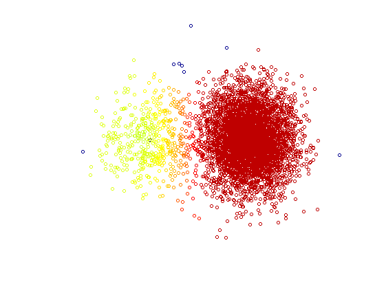
where is a -dimensional Brownian motion and is a temperature parameter controlling the amount of noise introduced in the gradient flow. We use the gradient of the logarithm of here as this quantity arises naturally in practice. Indeed, since we only have access to a discretization of the space through the sampled data points, we mimic this perturbed gradient flow by a random walk on the data points. Ting et al. [18] proved an isotropic random walk on a neighborhood graph approximates the previous diffusion process for while other values of are obtained by putting weights on the edges of the graph. At this point, one could perform fuzzy clustering by considering the first local maximum of the density encountered by the random walk, an approach wich has been proposed by Chen et al. [7]. However, as emphasized by Luxburg et al. [17], the hitting time to a single point for a random walk on the graph converges to irrelevant quantities when the number of data points goes to infinity. We can thus expect the clustering to fail in that case. Indeed, if we apply this method to the fuzzy clustering of two different Gaussian measures (see Figure 1). The obtained fuzzy memberships are unsatisfying. In order to circumvent this issue, we assign a zone of high density to each cluster, called cluster core and computed using the mode-seeking (hard) clustering algorithm ToMATo [5]. The fuzzy membership of a point to a given cluster is then given by the probability for the random walk started at this point to hit the corresponding cluster core first.
2 The Algorithm
Our algorithm is a fuzzy generalization of the ToMATo algorithm which relies on the concept of . Let be a graph and be a real valued function on the vertices of this graph. For any , let be the -superlevel-set of . A new connected component is born in when reaches a local maximum of on and we denote by the corresponding value of . This component then dies at when it gets connected, in , to another connected component such that . The prominence of (and by extension, of the corresponding local maximum of ) is then simply .
The algorithm takes as input a finite set of points together with pairwise distances . In practice only the distances are used, so there is no need for point coordinates. Additionally, the algorithm takes in the following set of parameters:
- •
a density estimator ,
- •
a kernel , for example the Gaussian kernel,
- •
a window size ,
- •
a prominence threshold ,
- •
a temperature .
The first four parameters are in fact required by ToMATo for hard mode-seeking, upon which our algorithm relies. The last parameter is the one added in for fuzzy mode-seeking, as per Equation (1).
Given this input, our algorithm proceeds as follows:
- 1.
It builds a weighted neighborhood graph on top of the point cloud , adding an edge with weight
(2) between each pair of points . Remark that it is possible to replace our kernel-based graph by a nearest neighbour graph.
- 2.
It computes the cluster cores by running ToMATo with input , , , and the unweighted neighborhood graph obtained from by removing the edges with weights lower than . The output of ToMATo is a set of clusters . Each cluster corresponds to the basin of attraction of some peak of of prominence at least within . Up to a reordering of the data points, we can assume this peak to be . The -th cluster core is then taken to be the highest and most stable part of , defined formally as the connected component containing within the subgraph of spanned by those vertices such that .
- 3.
It computes the fuzzy-membership values by solving the linear system , where the matrix is defined by:
where is the transition kernel of the random walk on the graph, i.e.
(3)
The output of the algorithm is the set of fuzzy-membership values computed at step 3.
3 Parameters selection
3.1 Density estimator, window size, kernel and prominence threshold
These parameters are tied to the classical hard mode-seeking framework. The density estimator can be linked to the window size in practice, as is done e.g. in Mean-Shift [10] and its successors. For instance, one can consider the kernel density estimator associated to the kernel . This not only reduces the number of parameters to tune in practice, but it also gives a way to select using standard parameter selection techniques for density estimation, which is done for example in [7]. Finally, the prominence threshold is used to distinguish between relevant and irrelevant peaks in the discrete setting. It can be selected by running ToMATo twice: once to get the distribution of prominences of the peaks of within the neighborhood graph , from which can be inferred by looking for a gap in the distribution; then a second time, using the chosen value of , to get the final hard clustering. This procedure is detailed in Chazal et al. [5].
3.2 Temperature parameter
This parameter is standard in fuzzy clustering. Outputs corresponding to large values of will tend to have smooth interfaces between clusters, while small values of will encourage quick transitions from one cluster to another. can also be interpreted as a trade-off between the respective influence of the metric and of the density in the diffusion process: when is small, the output of our algorithm is mostly guided by the density and therefore close to the output of mode seeking algorithms; by contrast, when is large, the algorithm becomes oblivious to the density. In practice, one may get insights into the choice of by looking at the evolution of a certain measure of fuzziness of the output clustering across a range of values of . We elaborate on this in Section 5.
4 Convergence guarantees
In this section we provide guarantees to our fuzzy clustering scheme by exploiting the convergence of the random walk over the neighborhood graph to a continuous diffusion process.
As is usual in mode-seeking, we assume our input data points to be i.i.d random variables drawn from some unknown probability density over . We also assume that the metric that equips the data points is the Euclidean norm, and that satisfies the following technical conditions:
- •
is Lipschitz continuous over and -continuous over the domain ,
- •
,
- •
The SDE 1 is well-posed.
Standard sufficient conditions ensuring the well-posedness (particularly the non-explosion) of the SDE 1 can be found in Albeverio et al. [1] or in Krylov and Röckner [16], for example one can assume to be Lipschitz continuous.
Our analysis connects random walks on graphs built on top of the input point cloud using a density estimator to the solution of Equation 1, for a fixed temperature parameter . Specifically, let denote the Markov Chain whose initial state is the closest neighbour of in the point cloud (break ties arbitrarily), and whose transition kernel is given by Equation 3. Following the approach of Ting et al. [18], we show that, under suitable conditions on the estimator , this graph-based random walk approximates the diffusion process in the continuous domain in the following sense: there exists depending on such that, as tends to infinity, with high probability, converges weakly to the solution of Equation (1). From there, under standard conditions for mode estimation on the window size and on the density estimator (see [8, 2]), we obtain the convergence of the fuzzy-membership values computed by the algorithm to the membership defined from the underlying continuous diffusion process . Formally, letting be the local maxima of of prominence higher than , and , their associated cluster cores in the continuous domain (i.e. is the connected component containing in ), we define as the probability for the diffusion process solution of (1) to hit before any other .
Theorem 1.
Let and assume is bounded from below on the boundary of the underlying cluster cores . Let be a decreasing window size such that while . Suppose the density estimator satisfies, for any compact set and any ,
Then, for any compact set , any and any ,
5 Experiments
We first illustrate the effect of the temperature parameter on the clustering output using synthetic data. We then apply our method on a couple UCI repository datasets and on simulated protein conformations data. In all our experiments we use a -nearest neighbor graph along with a distance to measure density estimator [4] computed using the nearest-neighbors.
5.1 Synthetic data
The first dataset is presented in Figure 2(a) and is composed of two high-density clusters connected by two links. The bottom link is sampled from a uniform density while the top link is sampled from a density that has a gap inbetween the two clusters. Standard mode seeking algorithms will have a hard time clustering the bottom link as a density estimation can create many “noisy” local maxima: for instance, ToMATo missclusters most of the bottom link (see Figure 2(b)). We display the results of our algorithm for three values of in Figure 2(c), in Figure 2(d) and in Figure 2(e). As we can see from the output of the algorithm, for small values of , the amount of noise injected in our trajectory is not large enough to compensate for the influence of the noise in the density estimation, so the result obtained is really close to hard clustering. Large values of do not give enough weight to the density function which leads to a smooth transition between the two clusters on the top link. Intermediate values of seem to give more satisfying results. In order to gain intuition regarding which value of one should use, it is possible to look at the evolution of a fuzziness value for the clustering. For example, one can consider a notion of clustering entropy:
| (4) |
which gets lower when the fuzziness of the clustering increases. As we can see in Figure 2(f), the evolution of with respect to presents three distincts plateaus corresponding to the three behaviour highlighted earlier.


The second dataset we consider is composed of two interleaved spirals—see Figure 3. An interesting property of this dataset is that the head of each spiral is close (in Euclidean distance) to the tail of the other spiral. Thus, the two clusters are well-separated by a density gap but not by the Euclidean metric. We use our algorithm with two different values of : and . We also run the spectral fuzzy-C means on a subsampling of this dataset. The first thing we want to emphasize is that the result of spectral clustering and our algorithm using are similar, this is to be expected as both algorithms rely on properties of the same diffusion operator, this also means that other fuzzy clustering techniques based on spectral clustering will fail on this dataset. Moreover, we can see that for , the density gap between the two spirals is not strong enough to compensate for the proximity of the two clusters in the Euclidean metric. On the other hand, for we recover the two clusters as we give more weight to the density structure.


5.2 UCI datasets
In order to obtain quantitative results regarding our fuzzy clustering scheme, we evaluate it in a classification scenario on a few datasets from the UCI repository: the Pendigits dataset ( points and clusters), the Waveset dataset ( points and clusters) and the Statlog dataset ( points for clusters). We preprocess each dataset by renormalizing the various coordinates so they have unit variance. Then, for each dataset, we run our algorithm with various values of the parameter between and , but a single value of and (given by a prominence gap), along with the fuzzy C-means algorithm for fuzziness parameters between and . We also consider the fuzzy clustering algorithm proposed by Chen et al. [7], for which the cluster cores are reduced to a single point. Let denote our sample points and their respective labels taking values in . In these datasets, there are only two plateaus, thus we choose . Thus, we propose an automatic selection of by computing the values of the clustering entropy for multiple values of and by selecting
in other words we take inbetween the two plateaus by choosing the value of maximizing the slope of . In order to evaluate hard clustering algorithms, it is common to use the purity measure defined by
where is a map from the set of clusters to the set of labels . As this measure is not adapted to fuzzy clustering, we define the -entropic purity as
for some . The parameter is used to prevent the quantity from exploding due to possible outliers. This extension of the traditional purity can be useful to evaluate fuzzy clustering as it can be seen as an approximation of which enjoys the following property.
Proposition 2.
Suppose that and let , then
Thus, for small values of , a fuzzy clustering minimizing the -entropic purity recovers the conditional probabilities of the labels with respect to the coordinates.
We provide the best -entropic purity obtained by each algorithm on all datasets in Table 1. As we can see, our algorithm outperforms the other fuzzy clustering algorithms on these datasets. In particular we can see that the simple fuzzy mode-seeking algorithm of Chen et al. [7] fails on the Waveform dataset.
| Algorithm / Data | Waveform | Pendigits | Statlog |
|---|---|---|---|
| Ours, optimal | -1.1 | -0.61 | -0.51 |
| Ours, automatic | -1.1 | -0.64 | -0.55 |
| Fuzzy C-means | -1.1 | -1.35 | -0.57 |
| Chen et al. [7] | -3.2 | -0.76 | -0.58 |
Alanine dipeptide conformations.
We now turn to the problem of clustering protein conformations. We consider the case of the alanine-dipeptide molecule. Our dataset is composed of protein conformations, each one represented as a -dimensional vector. The metric used on this type of data is the root-mean-squared deviation (RMSD). The goal of fuzzy clustering in this case is twofold: first, to find the right number of clusters corresponding to metastable states of the molecule; second, to find the conformations lying at the border between different clusters, as these represent the transition phases between metasable states. It is well-known that the conformations of alanine-dipeptide only have two relevant degrees of freedom, so it is possible to project the data down to two dimensions (called a Ramachadran plot) to have a comfortable view of the clustering output. See Figure 4 for an illustration, and note that the clustering is performed in the original space. In order to highlight interfaces between clusters, we only display the second highest membership function. As we can see there are clusters and to interfaces.


6 Proofs
6.1 Background on diffusion processes
Convergence of Markov chains to diffusion processes occurs in the Skorokhod space , composed of the trajectories that are right-continuous and have left limits, for some fixed . It is equipped with the following metric:
where denotes the space of strictly increasing automorphisms on the unit segment , and where is the quantity:
In diffusion approximation, standard results prove the weak convergence of a Markov chain to a difussion process in . A stochastic process converges weakly to a diffusion process in as tends to if and only if
| (5) |
for any Borel set such that .
Let us state the convergence result when is the Solution of the Stochastic Differential Equation 1. For this case, and . Consider a family of Markov chains defined on discrete state spaces , transition kernels and initial states . For and , let
- •
- •
- •
where is the complementary of the ball of radius centered at .
Proposition 3 (Adapted from Theorem 7.1 in [14]).
Let be a compact subset of . Let also be a Borel set in for some such that for all . For any , there exist parameters and such that
whenever the following conditions are met:
- (i)
- (ii)
- (iii)
- (iv)
6.2 Weak-Convergence
In this section, we prove the following result.
Proposition 4.
Let be the diffusion process solution of the SDE 1. Let be a decreasing function such that and . Suppose our estimator satisfies, for any compact set and any ,
Then, for any , for any compact set , and for any Borel set of such that for all , there exists a constant depending on such that for , we have
The proof relies on Theorem 3 of Ting et al. (2010) along with a proper control of boundary effects. Let and be strictly positive real numbers, throughout the course of the proof, the notation stands for the continuous time process . We denote by the i.i.d sampling which is also the state space of . For , let be the superlevel-set of and be trajectories staying in up to time . Since does not explode in finite time, there exists such that, for any , . To obtain a good approximation of the trajectories of staying in using , we only need to check assumptions (i)-(iv) of Proposition 3 on . is closed as is continuous and it is also bounded as , it is therefore compact. Applying Theorem 3 from Ting et al. (2010) on the points of the compact set , we have, with probability ,
- (i)
- (ii)
- (iii)
- (iv)
Thus, the assumptions (i)-(iv) of Proposition 3 are verified on .
Since is continuous, is an open set. Therefore, there exists such that for any ,
Therefore, for any Borel set ,
Thus, we only need to approximate trajectories that do not leave to obtain a good approximation of . So we can apply Corollary 3 on these trajectories with an accuracy of to obtain,
Every step of the proof hold almost surely as tends to infinity, thus the proof of Proposition 4 is complete.
6.3 Proof of Theorem 1
Let and be strictly positive real numbers and let be a compact set. Let be the cluster cores used by the algorithm and computed with the density estimator . These cluster cores are approximations of the sets obtained using the same computation with the true density . Since, by assumptions, is -continuous on and is non-zero on the boundary of the , we have
-
The are compact sets of that are well-separated (i.e. for all ).
-
For each , the boundary of is smooth.
By our assumptions on the convergence of along with Theorem 10.1 of [5],
| (6) |
where and .
Without loss of generality, we can assume that has a single connected component. Let be a strictly positive real and consider , we let
- •
be the probability that hits before any other ,
- •
be the probability that hits before any other .
Let us show that, for any , a trajectory entering has a high probability to enter if is small enough. Since the are closed and disjoint there exists such that the are disjoints. Moreover, since the have smooth boundaries, there exists such that if then, the probability for to hit before exiting is at least .
Similarly, if a trajectory enters , then it enters with high probability. More precisely there exists such that if a trajectory hits , then it hits with probability at least .
Let , by combining our results and using the strong Markov property of we obtain that:
- •
,
- •
.
The next step is to show that the approximation of provided by the Markov chain is correct. For , let
We define the stopping time
Since and has a single connected component, we have that , in particular that means that there exists such that for any , . Using Proposition 4, we have that, almost surely
Hence, we have
Since , we can apply Proposition 4 on the set , and obtain
Combined with our previous result, we obtain:
Using our assumption on , we have . Therefore, using our previous bound between and :
Similarly,
concluding the proof.
7 Conclusion
We have provided a fuzzy clustering algorithm based on the mode-seeking framework relying on the approximation of a diffusion process through the use of a random walk. Despite the convergence issues of random-walk-based quantities for large data highlighted by Luxburg et al. [17], we have shown that our algorithm does converge to meaningful values. Our thereotical result is backed up by encouraging experiments. The main question still open regarding our algorithm is the choice of the temperature parameter , while we have shown that the evolution of a quantification of the fuzziness of the clustering through the clustering entropy can give some hint about a correct choice for this parameter, it is not clear whether this can be done in all cases and for more complicated datasets.
Acknowledgements.
The authors wish to thank Cecilia Clementi and her student Wenwei Zheng for providing the alanine-dipeptide conformation data used in Figure 4. This work was supported by the French Délégation Générale de l’Armement (DGA), by ANR project TopData ANR-13-BS01-0008 and by ERC grant Gudhi (ERC-2013-ADG-339025).
References
- [1] Sergio Albeverio, Yuri Kondratiev, and Michael Röckner. Strong feller properties for distorted brownian motion and applications to finite particle systems with singular interactions. In Finite and infinite dimensional analysis in honor of Leonard Gross (New Orleans, LA, 2001), volume 317 of Contemp. Math., pages 15–35. Amer. Math. Soc., Providence, RI, 2003.
- [2] E. Arias-Castro, D. Mason, and B. Pelletier. On the estimation of the gradient lines of a density and the consistency of the mean-shift algorithm. Unpublished, 2013.
- [3] M. Azizyan, Y.-C. Chen, A. Singh, and L. Wasserman. Risk Bounds For Mode Clustering. ArXiv e-prints, May 2015.
- [4] G. Biau, F. Chazal, D. Cohen-Steiner, L. Devroye, and C. Rodriguez. A weighted k-nearest neighbor density estimate for geometric inference. Electronic Journal of Statistics, 5:204–237, 2011. URL https://hal.archives-ouvertes.fr/hal-00606482. http://imstat.org/ejs/.
- [5] Frédéric Chazal, Leonidas J. Guibas, Steve Y. Oudot, and Primoz Skraba. Persistence-based clustering in riemannian manifolds. J. ACM, 60(6):41, 2013. URL http://dblp.uni-trier.de/db/journals/jacm/jacm60.html#ChazalGOS13.
- [6] Y.-C. Chen, C. R. Genovese, R. J. Tibshirani, and L. Wasserman. Nonparametric Modal Regression. ArXiv e-prints, to appears in Annals of Statistics, December 2014a.
- [7] Y.-C. Chen, C. R. Genovese, and L. Wasserman. A Comprehensive Approach to Mode Clustering. ArXiv e-prints, to appears in Electronic Journal of Statistics, June 2014b.
- [8] Y.-C. Chen, C. R. Genovese, and L. Wasserman. Statistical Inference using the Morse-Smale Complex. ArXiv e-prints, June 2015a.
- [9] Y.-C. Chen, C. R. Genovese, and L. Wasserman. Density Level Sets: Asymptotics, Inference, and Visualization. ArXiv e-prints, April 2015b.
- [10] Yizong Cheng. Mean shift, mode seeking, and clustering. IEEE Trans. Pattern Anal. Mach. Intell., 17(8):790–799, August 1995. ISSN 0162-8828. doi: 10.1109/34.400568. URL http://dx.doi.org/10.1109/34.400568.
- [11] Minsu Cho and Kyoung Mu Lee. Authority-shift clustering: Hierarchical clustering by authority seeking on graphs. In CVPR, pages 3193–3200. IEEE, 2010. URL http://dblp.uni-trier.de/db/conf/cvpr/cvpr2010.html#ChoL10.
- [12] John D. Chodera, William C. Swope, Jed W. Pitera, and Ken A. Dill. Long-time protein folding dynamics from short-time molecular dynamics simulations. Multiscale Modeling & Simulation, 5(4):1214–1226, 2006. doi: 10.1137/06065146X. URL http://link.aip.org/link/?MMS/5/1214/1.
- [13] Dorin Comaniciu and Peter Meer. Mean shift: A robust approach toward feature space analysis. Pattern Analysis and Machine Intelligence, IEEE Transactions on, 24(5):603–619, 2002.
- [14] Richard Durrett. Stochastic calculus : a practical introduction. Probability and stochastics series. CRC Press, 1996.
- [15] W.L.G. Koontz, P.M. Narendra, and K. Fukunaga. A graph-theoretic approach to nonparametric cluster analysis. IEEE Transactions on Computers, 25(9):936–944, 1976. ISSN 0018-9340. doi: http://doi.ieeecomputersociety.org/10.1109/TC.1976.1674719.
- [16] N.V. Krylov and M. Röckner. Strong solutions of stochastic equations with singular time dependent drift. Probab. Theory Relat. Fields, 131(2):154–196, 2005.
- [17] Ulrike V. Luxburg, Agnes Radl, and Matthias Hein. Getting lost in space: Large sample analysis of the resistance distance. In Advances in Neural Information Processing Systems 23, pages 2622–2630. 2010.
- [18] Daniel Ting, Ling Huang, and Michael I. Jordan. An analysis of the convergence of graph laplacians. In ICML, 2010.