跳到论文正文
W Papers独立论文阅读器 arXiv:1406.6889 论文正文 计算阅读时间 · 0%
引用这篇论文根据当前论文元数据生成,正式投稿前建议核对。


License: arXiv.org perpetual non-exclusive license
arXiv:1406.6889v2 [cs.CG] 10 Jul 2014

Non-cooperative algorithms in self-assembly

Pierre-Etienne Meunier ††thanks: Aix Marseille Université, CNRS, LIF UMR 7279, 13288, Marseille, France, pierre-etienne.meunier@lif.univ-mrs.fr. Supported in part by National Science Foundation Grant CCF-1219274.
Abstract

We show the first non-trivial positive algorithmic results (i.e. programs whose output is larger than their size), in a model of self-assembly that has so far resisted many attempts of formal analysis or programming: the planar non-cooperative variant of Winfree’s abstract Tile Assembly Model.

This model has been the center of several open problems and conjectures in the last fifteen years, and the first fully general results on its computational power were only proven recently (SODA 2014). These results, as well as ours, exemplify the intricate connections between computation and geometry that can occur in self-assembly.

In this model, tiles can stick to an existing assembly as soon as one of their sides matches the existing assembly. This feature contrasts with the general cooperative model, where it can be required that tiles match on several of their sides in order to bind.

In order to describe our algorithms, we also introduce a generalization of regular expressions called baggins expression . Finally, we compare this model to other automata-theoretic models.

1 Introduction

Self-assembly is the process by which unorganized atomic components coalesce into complex shapes and structures in an unsupervised way. This kind of processes is ubiquitous in nature, and in particular in the complex molecular components of life. In recent years, its study has yielded a growing number of impressive experimental realizations, ranging from regular arrays [30] to fractal structures [23, 11], smiling faces [21, 28], DNA tweezers [31], logic circuits [24, 19], neural networks [20], and molecular robots[15].

Potential future applications range from more efficient, cheaper computational units to interactions with natural biological processes, both for medical diagnosis and treatment, and a better understanding of evolution and development.

Realizing that programming these processes is the keystone of atomically precise molecular engineering, Winfree introduced in 1998 the abstract Tile Assembly Model [29] to program assemblies using the components built by Seeman [25] using DNA. This model is similar to Wang tilings [27], essentially augmented with a mechanism for sequential growth, and thus allowing mismatches between adjacent tiles. More precisely, in the abstract Tile Assembly Model, we consider square tiles from a finite set of types, with colors and integer glue strengths on each side. The assembly starts from a single “seed” tile, and proceeds by adding one tile at a time, asynchronously and nondeterministically. At each step, a tile can stick to the current assembly if the glue strengths, on its sides whose colors match the current assembly, sum up to at least a parameter of the model called the temperature τ=1,2,3​…\tau=1,2,3\ldots

In the present work, we are mostly interested in the case of temperature 1 self-assembly, also called non-cooperative self-assembly. In the abstract Tile Assembly Model, when the temperature increases, fewer assemblies are possible, allowing more control over producible assemblies: for instance, cooperative self-assembly (i.e. at temperature at least 2) is able to simulate arbitrary Turing machines [29, 22, 14], and produce arbitrary connected shapes with a number of tile types within a log factor of their Kolmogorov complexity [26]. More surprisingly, this model has even been shown intrinsically universal [8], meaning that there is a single tileset capable of simulating arbitrary tile assembly systems, modulo rescaling, even with a single tile type [6].

Despite its apparent simplicity, the non-cooperative model is far from being well understood, and not known to be capable of general Turing computation. However, this is a fundamental and ubiquitous form of growth in nature, as many systems, from plants to mycelium to percolation processes, exhibit this kind of behavior by growing and branching tips.

In one of the first studies on self-assembly [22], Rothemund and Winfree conjectured it to be less powerful than cooperative self-assembly. The first fully general separation result, without unproven hypotheses, was only proven recently [18], in the context of intrinsic universality [9, 8, 7]. Before that, several results had shown separations between particular cases of the model [10, 3, 17], and general self-assembly.

One of the most puzzling results on this model is its capability to simulate Turing machines in the three dimensional generalization of the model [5], whereas in one dimension, it is equivalent to finite automata.

1.1 Main results

Here, we present the first efficient constructions in the fully general planar noncooperative model. The generally accepted definition of an “efficient program”, in this context, is a program whose output is larger than its size. Of course, a simple first result on this model shows that arbitrary shapes can be built with a number of tile types equal to the number of tiles in the shape, or (for simpler shapes) equal to the Manhattan diameter of the shape [22].

Surprisingly, our results show that there are tile assembly systems whose terminal assemblies are all larger (in Manhattan diameter) than their number of tile types. Although a number of terms have not been defined yet, we briefly introduce our two main constructions. The first construction can be proven easily by hand; we will demonstrate it first in Section 3.2, and then generalize it in Section 3.3, to get the following theorem:

Theorem 3.4.

For all integer nn, there is a tile assembly system 𝒯n=(Tn,σn,1)\mathcal{T}_{n}=(T_{n},\sigma_{n},1) such that |Tn|=n|T_{n}|=n, and for all terminal assembly a∈𝒜□​[𝒯n]a\in\mathcal{A}_{\Box}[{\mathcal{T}_{n}}], aa is finite and of height 2​n+o⁡(n)2n+o(n).

Intuitively, this construction works by preventing subpaths starting and ending with the same tile type to repeat completely. However, it does not address the possibility that some paths be efficient by repeating a subpath several times, before being blocked. Since these partial pumping have been a major puzzle of the field, we provide a second efficient construction allowing it.

However, its proof is significantly more complicated, and a generalized form of our construction does not seem easy. In Section 3.4, we present the computer-aided proof of its efficiency, that we have needed due to the size at which the first “savings” of tile types are seen. Computer-aided proofs are of growing importance in computer science and mathematics, as exemplified by its latest developments in complexity theory, also in the context of tile assembly [13].

However, our case here is significantly simpler, since this construction could be verified by hand, probably within a few hours:

Theorem 3.5.

There is a tile assembly system 𝒯=(T,σ,1)\mathcal{T}=(T,\sigma,1) such that |dom⁡(σ)|=1|{\rm dom}(\sigma)|=1, and all terminal assemblies of 𝒯\mathcal{T} contain a path PP of Manhattan diameter strictly larger than |T|+1|T|+1, that is partially pumped, i.e. parts of PP are consecutive repetitions of one of its subpath.

Finally, we compare this model, and several generalizations of it, to various models of automata: finite automata, tree automata, and pushdown automata. These models are explained in Section 4, and the comparison is summarized on Figure 5.

1.2 Key technical ideas and methods

A major challenge, when studying non-cooperative self-assembly, is to overcome the intuition given by the one-dimensional case (which is equivalent to finite automata), that any repetition of a tile type may allow to “pump” an assembly. Indeed, an easy observation shows that assemblies formed at temperature 1 are nothing more than a collection of paths growing from the seed: if a tile type is ever repeated along a path, it is tempting to try to repeat the subpath between these repetitions.

However, geometry makes things more complex. First, there are simple counter-examples to this pumping idea. Moreover, paths could first lay “blocking parts” out, and then come back and branch to check which type of blocker has been formed; this is for instance the primary mechanism used by the simulation of Turing machines in 3d shown in [5]. However, their construction “fakes cooperation” by laying a blocker out for all alternatives but one.

On the other hand, recent (unpublished) progresses tend to show that this kind of “bit reading” gadgets is not possible in two dimensions. This model thus asks a different question: can you write efficient programs without the ability to read your workspace?

Our results show that this is possible, at least to some extent. They do so by carefully considering the fact that paths that are monotonic in one dimension are pumpable; therefore, we must build “caves”, i.e. subpaths that are non-monotonic in both dimensions. However, since these are more expensive to build than straight paths, we also need to reuse these extra tile types several times, either by making these subpaths self-blocking (in Section 3.3), and branching before the blocking, or by allowing some pumping (in Section 3.4) before blocking it.

These results are quite puzzling and counter-intuitive; however, they do not seem to make Turing computation possible. Therefore, a natural question is the exact power of this model, that depends strongly on geometry, and that no other “classical” model seems to capture, as shown in Section 4.

2 Definitions and preliminaries

We begin by defining the abstract tile assembly model, in a slightly more general framework than usually. Let GG be a group with nn generators i0→,i1→,…,in−1→\overrightarrow{i_{0}},\overrightarrow{i_{1}},\ldots,\overrightarrow{i_{n-1}}, and arbitrary relators. We will use GG to define the geometric space: for instance, ℤ2\mathbb{Z}^{2} has two generators i0→=(1,0)\overrightarrow{i_{0}}=(1,0) and i1→=(0,1)\overrightarrow{i_{1}}=(0,1), and one relation i0→​i1→=i1→​i0→\overrightarrow{i_{0}}\overrightarrow{i_{1}}=\overrightarrow{i_{1}}\overrightarrow{i_{0}}.

A tile type is a unit square with 2​n2n sides, each consisting of a glue label and a nonnegative integer strength. In the most common case where n=2n=2, we call a tile’s sides north, east, south, and west, respectively, according to the following picture:

i0→\overrightarrow{i_{0}} (East)i1→\overrightarrow{i_{1}} (North)−i0→-\overrightarrow{i_{0}} (West)−i1→-\overrightarrow{i_{1}} (South)

Also, we write these directions N\mathrm{N}, E\mathrm{E}, S\mathrm{S} and W\mathrm{W}, respectively. When there is no ambiguity, we also write N⁡(t)\mathrm{N}(t), E⁡(t)\mathrm{E}(t), S⁡(t)\mathrm{S}(t) and W⁡(t)\mathrm{W}(t), to mean the north, east, south and west glue of tile type tt, respectively. Moreover, for each direction dd, we write −d-d its opposite direction. We assume a finite set TT of tile types, but an infinite supply of copies of each type. An assembly is a positioning of the tiles on the Cayley graph of GG, that is, a partial function α:G⇢T\alpha:G\dashrightarrow T. To simplify the notations, we will assume G=ℤ2G=\mathbb{Z}^{2} throughout the paper, unless explicitly mentioned.

In this context, we say that two elements g0,g1∈Gg_{0},g_{1}\in G are adjacent if g1=g0+ik→g_{1}=g_{0}+\overrightarrow{i_{k}} (respectively g1=g0−ik→g_{1}=g_{0}-\overrightarrow{i_{k}}) for some generator ik→\overrightarrow{i_{k}}. In this case, their abutting side is the ik→\overrightarrow{i_{k}} side (respectively the −ik→-\overrightarrow{i_{k}} side) of g0g_{0}, and the −ik→-\overrightarrow{i_{k}} side (respectively the ik→\overrightarrow{i_{k}} side) of g1g_{1}.

We say that two tiles in an assembly interact, or are stably attached, if the glue labels on their abutting side are equal, and have positive strength. An assembly α\alpha induces a weighted binding graph Gα=(Vα,Eα)G_{\alpha}=(V_{\alpha},E_{\alpha}), where Vα=dom⁡(α)V_{\alpha}={\rm dom}(\alpha) (the domain of α\alpha), and there is an edge (a,b)∈Eα(a,b)\in E_{\alpha} if and only if aa and bb interact, and this edge is weighted by the glue strength of that interaction. The assembly is said to be τ\tau-stable if any cut of GαG_{\alpha} has weight at least τ\tau.

A tile assembly system is a triple 𝒯=(T,σ,τ)\mathcal{T}=(T,\sigma,\tau), where TT is a finite tile set, σ\sigma is called the seed, and τ\tau is the temperature. Throughout this paper, we will always have τ=1\tau=1, and σ\sigma will always be an assembly with exactly one tile. Therefore, we can make the simplifying assumption that all glues have strength one without changing the behavior of the model.

Given two τ\tau-stable assemblies α\alpha and β\beta, we say that α\alpha is a subassembly of β\beta, and write α⊑β\alpha\sqsubseteq\beta, if dom⁡(α)⊆dom⁡(β){\rm dom}(\alpha)\subseteq{\rm dom}(\beta) and for all p∈dom⁡(α)p\in{\rm dom}(\alpha), α⁡(p)=β⁡(p)\alpha(p)=\beta(p). We also write α→1𝒯β\alpha\rightarrow_{1}^{\mathcal{T}}\beta if we can get β\beta from α\alpha by the binding of a single tile, that is, if α⊑β\alpha\sqsubseteq\beta and |dom⁡(β)∖dom⁡(α)|=1|{\rm dom}(\beta)\setminus{\rm dom}(\alpha)|=1. We say that γ\gamma is producible from α\alpha, and write α→𝒯γ\alpha\rightarrow^{\mathcal{T}}\gamma if there is a (possibly empty) sequence α=α1,…,αn=γ\alpha=\alpha_{1},\ldots,\alpha_{n}=\gamma such that α1→1𝒯…→1𝒯αn\alpha_{1}\rightarrow_{1}^{\mathcal{T}}\ldots\rightarrow_{1}^{\mathcal{T}}\alpha_{n}.

A sequence of k∈ℤ+∪{∞}k\in\mathbb{Z}^{+}\cup\{\infty\} assemblies α0,α1,…\alpha_{0},\alpha_{1},\ldots over 𝒜T\mathcal{A}^{T} is a 𝒯\mathcal{T}-assembly sequence if, for all 1≤i<k1\leq i<k, αi−1→1𝒯αi\alpha_{i-1}\to_{1}^{\mathcal{T}}\alpha_{i}.

The set of productions of a tile assembly system 𝒯=(T,σ,τ)\mathcal{T}=(T,\sigma,\tau), written 𝒜⁡[𝒯]\mathcal{A}[{\mathcal{T}}], is the set of all assemblies producible from σ\sigma. An assembly α\alpha is called terminal if there is no β\beta such that α→1𝒯β\alpha\rightarrow_{1}^{\mathcal{T}}\beta. The set of terminal assemblies is written 𝒜□​[𝒯]\mathcal{A}_{\Box}[{\mathcal{T}}].

The Manhattan distance ‖A​B→‖1\|\overrightarrow{AB}\|_{1} between two points A=(xA,yA)A=(x_{A},y_{A}) and B=(xB,yB)B=(x_{B},y_{B}) is ‖A​B→‖1=|xA−xB|+|yA−yB|\|\overrightarrow{AB}\|_{1}=|x_{A}-x_{B}|+|y_{A}-y_{B}|. The Manhattan diameter of a connected assembly is the maximal Manhattan distance between two points in the assembly. We write (un)n∈ℕ(u_{n})_{n\in\mathbb{N}} to mean “the infinite sequence u0u_{0}, u1u_{1}, u2u_{2}, …\ldots”.

A regular tree grammar G=(S,N,ℱ,R)G=(S,N,\mathcal{F},R), according to [4], is given by an axiom SS, a set NN of nonterminal symbols, a set ℱ\mathcal{F} of terminal symbols, and a set RR of production rules of the form A→βA\rightarrow\beta where AA is a nonterminal and β\beta is a tree whose nodes are labeled by elements of ℱ∪N\mathcal{F}\cup N. Moreover, it is required that ℱ∩N=∅\mathcal{F}\cap N=\emptyset. In this work, we write trees as “nested function applications”: for instance, f⁡(x,g⁡(y,z))f(x,g(y,z)) is the following tree:

xxyyzzggff

The classical example of a regular tree grammar is the grammar of lists of integers, with one axiom L​i​s​tList, non-terminals L​i​s​tList and N​a​tNat, terminals 00, n​i​lnil, s⁡()s() and cons(,)cons(,), and the following rules:

L​i​s​t\displaystyle List →\displaystyle\rightarrow n​i​l\displaystyle nil
L​i​s​t\displaystyle List →\displaystyle\rightarrow c​o​n​s​(N​a​t,L​i​s​t)\displaystyle cons(Nat,List)
N​a​t\displaystyle Nat →\displaystyle\rightarrow 0\displaystyle 0
N​a​t\displaystyle Nat →\displaystyle\rightarrow s⁡(N​a​t)\displaystyle s(Nat)

3 Efficient algorithms

In this section, we show the main ideas of our efficient tileset. In order to describe them unambiguously, we use two different tools: figures showing the complete tileset and seed on the one hand, and programs written in a generalization of regular expressions called baggins expressions. An implementation of these expressions using a “sublanguage” of Haskell (i.e. a monad) is available at http://hackage.haskell.org/package/Baggins.

Moreover, all the constructions of this paper were generated in this language, and their source code is available on the self-assembly wiki11 1 http://self-assembly.net/wiki/index.php?title=Baggins-expressions .

3.1 Baggins expressions

A program in this language is an expr\mathrm{expr}, where expr\mathrm{expr} is defined by the following grammar (where an 𝑖𝑑𝑒𝑛𝑡𝑖𝑓𝑖𝑒𝑟\mathit{identifier} is a name):

expr\displaystyle\mathrm{expr} :⁣=\displaystyle:= atom|let|bind|from|expr;expr\displaystyle\mathrm{atom}\ |\ \mathrm{let}\ |\ \mathrm{bind}\ |\ \mathrm{from}\ |\ \mathrm{expr}\ \mathtt{;}\ \mathrm{expr}
atom\displaystyle\mathrm{atom} :⁣=\displaystyle:= 𝚖𝚘𝚟𝚎𝙽|𝚖𝚘𝚟𝚎𝙴​|𝚖𝚘𝚟𝚎𝚂|​𝚖𝚘𝚟𝚎𝚆\displaystyle\mathtt{moveN}\ |\ \mathtt{moveE}\ |\ \mathtt{moveS}\ |\ \mathtt{moveW}
let\displaystyle\mathrm{let} :⁣=\displaystyle:= 𝚕𝚎𝚝​𝑖𝑑𝑒𝑛𝑡𝑖𝑓𝑖𝑒𝑟\displaystyle\mathtt{let}\ \mathit{identifier}
bind\displaystyle\mathrm{bind} :⁣=\displaystyle:= 𝚋𝚒𝚗𝚍⁡[𝙽|𝙴​|𝚂|​𝚆]​𝑖𝑑𝑒𝑛𝑡𝑖𝑓𝑖𝑒𝑟\displaystyle\mathtt{bind}\ [\ \mathtt{N}\ |\ \mathtt{E}\ |\ \mathtt{S}\ |\ \mathtt{W}\ ]\ \mathit{identifier}
from\displaystyle\mathrm{from} :⁣=\displaystyle:= 𝚏𝚛𝚘𝚖​𝑖𝑑𝑒𝑛𝑡𝑖𝑓𝑖𝑒𝑟\displaystyle\mathtt{from}\ \mathit{identifier}
Definition 3.1.

Let ee be a baggins expression. Let β\beta the set of its identifiers. We define the unique tileset described by ee by induction on ee:

Let T0T_{0} be a tileset consisting of a unique tile type σ0\sigma_{0}, C0=σ0C_{0}=\sigma_{0} and α0\alpha_{0} is the function defined nowhere. Then, for all i∈{0,1,…,|e|−1}i\in\{0,1,\ldots,|e|-1\}:

  • •

    If ei=𝚖𝚘𝚟𝚎𝙽e_{i}=\mathtt{moveN}, Ci+1=(gN,gE,N⁡(Ci),gW)C_{i+1}=(g_{\mathrm{N}},g_{\mathrm{E}},\mathrm{N}(C_{i}),g_{\mathrm{W}}), and Ti+1=Ti∪{Ci+1}T_{i+1}=T_{i}\cup\{C_{i+1}\}, where gNg_{\mathrm{N}}, gEg_{\mathrm{E}}, gWg_{\mathrm{W}} are all new glues, not appearing on any tile of TiT_{i}. Moreover, let αi+1=α\alpha_{i+1}=\alpha.

  • •

    If ei=𝚖𝚘𝚟𝚎𝚂e_{i}=\mathtt{moveS}, Ci+1=(S⁡(Ci),gE,gS,gW)C_{i+1}=(\mathrm{S}(C_{i}),g_{\mathrm{E}},g_{\mathrm{S}},g_{\mathrm{W}}), and Ti+1=Ti∪{Ci+1}T_{i+1}=T_{i}\cup\{C_{i+1}\}, where gSg_{\mathrm{S}}, gEg_{\mathrm{E}}, gWg_{\mathrm{W}} are all new glues, not appearing on any tile of TiT_{i}. Moreover, let αi+1=α\alpha_{i+1}=\alpha.

  • •

    If ei=𝚖𝚘𝚟𝚎𝙴e_{i}=\mathtt{moveE}, Ci+1=(gN,W⁡(Ci),gS,gW)C_{i+1}=(g_{\mathrm{N}},\mathrm{W}(C_{i}),g_{\mathrm{S}},g_{\mathrm{W}}), and Ti+1=Ti∪{Ci+1}T_{i+1}=T_{i}\cup\{C_{i+1}\}, where gNg_{\mathrm{N}}, gSg_{\mathrm{S}}, gWg_{\mathrm{W}} are all new glues, not appearing on any tile of TiT_{i}. Moreover, let αi+1=α\alpha_{i+1}=\alpha.

  • •

    If ei=𝚖𝚘𝚟𝚎𝚆e_{i}=\mathtt{moveW}, Ci+1=(gN,gE,gS,E⁡(Ci))C_{i+1}=(g_{\mathrm{N}},g_{\mathrm{E}},g_{\mathrm{S}},\mathrm{E}(C_{i})), and Ti+1=Ti∪{Ci+1}T_{i+1}=T_{i}\cup\{C_{i+1}\}, where gNg_{\mathrm{N}}, gEg_{\mathrm{E}}, gSg_{\mathrm{S}} are all new glues, not appearing on any tile of TiT_{i}. Moreover, let αi+1=α\alpha_{i+1}=\alpha.

  • •

    If ei=𝚕𝚎𝚝​xe_{i}=\mathtt{let}\ x, then let αi+1\alpha_{i+1} be the function of domain dom⁡(αi)∪{x}{\rm dom}(\alpha_{i})\cup\{x\}, such that for all y∈dom⁡(αi)∖{x}y\in{\rm dom}(\alpha_{i})\setminus\{x\}, αi+1​(y)=αi​(y)\alpha_{i+1}(y)=\alpha_{i}(y), and αi+1​(x)=Ci\alpha_{i+1}(x)=C_{i}.

  • •

    If ei=𝚋𝚒𝚗𝚍​d​xe_{i}=\mathtt{bind}\ d\ x, where d∈{N,S,E,W}d\in\{\mathrm{N},\mathrm{S},\mathrm{E},\mathrm{W}\} and x∈αix\in\alpha_{i}, then:

    • –

      Ci+1=CiC_{i+1}=C_{i},

    • –

      αi+1=αi\alpha_{i+1}=\alpha_{i}, and

    • –

      let gg be the glue on side dd of CiC_{i}, and −g-g be the glue on side −d-d of αi​(x)\alpha_{i}(x). Then Ti+1T_{i+1} is TiT_{i} where all glues on sides dd and −d-d, that are equal to g′g^{\prime}, are replaced with gg.

  • •

    If ei=𝚏𝚛𝚘𝚖​xe_{i}=\mathtt{from}\ x, where x∈αix\in\alpha_{i}, let Ti+1=TiT_{i+1}=T_{i}, αi+1=αi\alpha_{i+1}=\alpha_{i}, and Ci=αi​(x)C_{i}=\alpha_{i}(x).

Theorem 3.2.

Definition 3.1 is “sound and complete”, i.e. any baggins expression describes exactly one tile assembly system, and any single-seeded tile assembly system can be described by a baggins expression.

Proof.

We prove the two properties independently:

  • •

    First remark that the construction of Definition 3.1 defines a tileset and a seed non-ambiguously.

  • •

    Now, let 𝒯=(T,σ,1)\mathcal{T}=(T,\sigma,1) be a temperature 1 tile assembly system with |dom⁡(σ)|=1|{\rm dom}(\sigma)|=1. Start with D={σ}D=\{\sigma\}. Then, for each tile t∈T∖Dt\in T\setminus D that can bind to a tile t0∈Dt_{0}\in D on side d∈{N,S,E,W}d\in\{\mathrm{N},\mathrm{S},\mathrm{E},\mathrm{W}\} of t0t_{0}, add 𝚏𝚛𝚘𝚖​t0​𝚖𝚘𝚟𝚎​d\mathtt{from}\ t_{0}\ \mathtt{move}d to DD. Also, from any previously created tile t1t_{1} that can bind to t0t_{0}, add 𝚏𝚛𝚘𝚖​t0​𝚋𝚒𝚗𝚍​d​t1\mathtt{from}\ t_{0}\ \mathtt{bind}\ d\ t_{1} to DD, if this binding has not been defined before, either directly or by operation 𝚏𝚛𝚘𝚖​t1​𝚋𝚒𝚗𝚍​(−d)​t1\mathtt{from}\ t_{1}\ \mathtt{bind}\ (-d)\ t_{1} (and do nothing else).

    Clearly, this baggins expression describes 𝒯\mathcal{T}, by Definition 3.1.

∎

In order to make the examples in the appendix shorter and more intuitive, the actual language used in our examples differs slightly from this grammar. However, all its instructions can clearly be written using baggins expression constructs.

3.2 A first efficient algorithm

In this section, we call a tile assembly system 𝒯=(T,σ,1)\mathcal{T}=(T,\sigma,1) efficient if there is an integer rr, such that the Manhattan diameter of all the terminal assemblies of 𝒯\mathcal{T} is strictly larger than |T|+|dom⁡(σ)||T|+|{\rm dom}(\sigma)|, and at most rr.

A simple observation on paths, is that any path that is monotonic in one dimension (i.e. the sequence (yPi)i(y_{P_{i}})_{i} of its y-coordinates, or the sequence (xPi)i(x_{P_{i}})_{i} of its x-coordinates is monotonic), and repeats a tile type, is pumpable.

Therefore, the main ingredient of efficient paths is non-monotonicity: we call a vertical cave (respectively horizontal cave) a part of a path PP between two indices ii and jj, such that (1) yPi=yPjy_{P_{i}}=y_{P_{j}}, (2) for all k<ik<i, yPk≤yPiy_{P_{k}}\leq y_{P_{i}}, and (3) for all k∈{i+1,i+2,…,j−1}k\in\{i+1,i+2,\ldots,j-1\}, yPk<yPiy_{P_{k}}<y_{P_{i}}.

Our first tile assembly system 𝒯0\mathcal{T}_{0} is presented completely in Appendix A, in the form of a baggins expression. We prove it now:

Theorem 3.3.

For all integer nn, there is a tile assembly system 𝒯n=(Tn,σn,1)\mathcal{T}_{n}=(T_{n},\sigma_{n},1) such that |Tn|=n|T_{n}|=n, and for all terminal assembly a∈𝒜□​[𝒯n]a\in\mathcal{A}_{\Box}[{\mathcal{T}_{n}}], aa is finite and of height 5​(n+2)4−23\frac{5(n+2)}{4}-23.

Proof.

Let T0T_{0} be the set of tiles appearing on the lower right assembly of Figure 1, and σ0\sigma_{0} be the upper left assembly of that figure.

This tileset has 38 tile types, and its terminal assemblies are of height 27; it is not efficient yet. But we will now add a number of new tile types to make it efficient. First replace the following glues (zoom in on Figure 1 to see these glue numbers, or see the large version in Appendix D):

  • •

    glue 6 by (6,0)(6,0) on the north, and (6,n)(6,n) on the south,

  • •

    glue 14 by (14,0)(14,0) on the north, and (14,n)(14,n) on the south,

  • •

    glue 24 by (24,0)(24,0) on the north, and (24,n)(24,n) on the south,

  • •

    glue 26 by (26,0)(26,0) on the north, and (26,n)(26,n) on the south,

And then for all i∈{6,14,24,26}i\in\{6,14,24,26\} and j∈{0,1,…,n−1}j\in\{0,1,\ldots,n-1\}, add a tile type to TT, with south glue (i,j)(i,j) and north glue (i,j+1)(i,j+1). In total, we have added 4​n4n tile types, but the terminal assemblies of TT grow 5​n5n higher. See Figure 2 for a larger example (saving tile type).

1
2019212022212322191818171716161598109111012111312141315361487121324354657326
201921202221232224232524191829302835292728262725261817303117163134354657326213422212322242325241615323334332835292728262725262237232224232524981091110121113121413153614351213121413153614373627282627252687121324354657326
2019212022212322242325241918293028352927282627252622372322242325241817303135121312141315361437362728262725261716313435465732621342221232224232524161522372322242325243233343328352927282627252622372322242325249810911101211131214131536143736272826272526351213121413153614373627282627252687121324354657326213422212322242325243233343328352927282627252622372322242325243512131214131536143736272826272526
Figure 1: Four successive stages of the construction: first the seed, then the main path grows, and finally, additional branches can also grow completely, along the main path.
3433353436353736383739384039414042414342444345444645333257585663575556545553545253515250514950484947484647366537363837393840394140424143424443454446453231585963192019212022212322242325242625272628272964286564555654555354525351525051495048494748464731305934354657687981091110121113121460133562363537363837393840394140424143424443454446453029366537363837393840394140424143424443454446456061626156635755565455535452535152505149504849474846473665373638373938403941404241434244434544464516151716181719182019212022212322242325242625272628272964286564555654555354525351525051495048494748464763192019212022212322242325242625272628272964286564555654555354525351525051495048494748464715141213243546576879810911101211131214601335623635373638373938403941404241434244434544464560616261566357555654555354525351525051495048494748464736653736383739384039414042414342444345444645631920192120222123222423252426252726282729642865645556545553545253515250514950484947484647
Figure 2: An efficient tile assembly system, producing an assembly of width 112 with 106 tile types. This terminal assembly grew from a seed containing only its leftmost tile.

∎

3.3 A more general scheme

In the construction of Theorem 3.3, repetitions of a tile type are done at the expense of width of the assembly: indeed, in order to avoid collisions between repeated paths, each repetition needs to be more and more narrow. Generalizing this remark yields the following Theorem:

Theorem 3.4.

For all integer nn, there is a tile assembly system 𝒯n=(Tn,σn,1)\mathcal{T}_{n}=(T_{n},\sigma_{n},1) such that |Tn|=n|T_{n}|=n, and for all terminal assembly a∈𝒜□​[𝒯n]a\in\mathcal{A}_{\Box}[{\mathcal{T}_{n}}], aa is finite and of height 2​n+o⁡(n)2n+o(n).

Proof.

The idea is to repeat the construction of Theorem 3.3 more than a constant number of times. A single cave, of height hh (see Figure 3), will be reused NN times, and at each iteration i∈{0,1,…,N}i\in\{0,1,\ldots,N\}, grow to height 2​h−i2h-i.

To do this, we use a sequence of assemblies as shown on Figure 3, with different widths (wn)n(w_{n})_{n}. The precise definition of this construction is given by the Haskell program in Appendix B, but the general idea is: grow some construction starting with tile type tt, then use some modification of the initial cave as a blocker, and then reuse tt.

hh
ttttwn=3n+3​nw_{n}=3^{n}+3n
Figure 3: The repeated part is shown on the left-hand side. The drawing on the right-hand side is a scheme of one step of the construction.

Then, we stack these parts on top of each other: on the Figure 4, the next assembly, drawn in dashed line, is of width wn−1=3n−1+3​(n−1)w_{n-1}=3^{n-1}+3(n-1). In order to avoid making a pumpable path, we do not grow the full initial cave each time, but a smaller and smaller suffix of it at each iteration.

Figure 4: Two successive iterations.

Because of this choice of widths, successive assemblies cannot collide with each other, and different repetitions of the same assembly cannot collide with each other either.

Let hh be the height of the initial cave. For all integer nn, the nt​hn^{th} repetition requires wn+2​wn−1≤2​wnw_{n}+2w_{n-1}\leq 2w_{n} new tiles horizontally, h−nh-n tiles vertically, and grows to a height of 2​(h−n)2(h-n). If we decide to repeat the construction N=log⁡hN=\log h times, we need |T|=2​∑i=1Nwn+N​h+O⁡(N2)|T|=2\sum_{i=1}^{N}w_{n}+Nh+O(N^{2}) tile types, i.e. h​log⁡h+O⁡(h)h\log h+O(h) tile types.

Moreover, in this case, all terminal assemblies will have height 2​h​log⁡h+O⁡(N2)2h\log h+O(N^{2}), which is 2​|T|+o⁡(|T|)2|T|+o(|T|).

The baggins expression for the exact construction is in Appendix B.

∎

3.4 Partially pumpable paths

The constructions of Sections 3.2 and 3.3 are efficient by repeating smaller and smaller parts of an assembly, while ensuring that the assembly does not become pumpable. The other way of building efficient paths is by letting them become pumpable for some time, after building structures that block these repetitions. However, blocking these parts is provably expensive, and the same kind of repeated blocking structure, similar to those of Sections 3.2 and 3.3, must be used to “save” tile types. However, this construction is intended as a proof that allowing some pumping still does not forbid the existence of efficient tilesets.

Theorem 3.5.

There is a tile assembly system 𝒯=(T,σ,1)\mathcal{T}=(T,\sigma,1) such that |dom⁡(σ)|=1|{\rm dom}(\sigma)|=1, and all terminal assemblies of 𝒯\mathcal{T} contain a path PP of Manhattan diameter strictly larger than |T|+1|T|+1, that is partially pumped, i.e. parts of PP are consecutive repetitions of one of its subpath.

Proof.

The smallest efficient tile assembly system that we found with a seed of size 1, has 4825 tile types, and all its terminal assemblies are of Manhattan radius 4845.

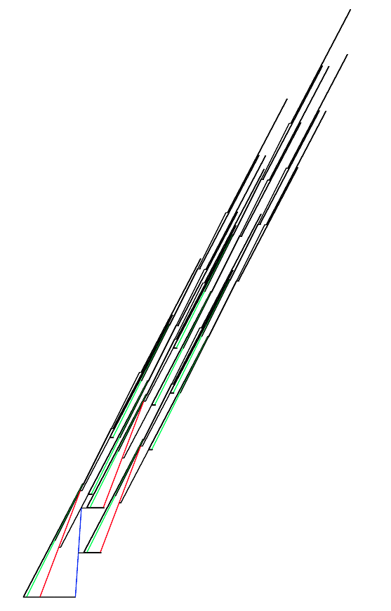
To show this, we use a computer-aided proof: more specifically, we simulate the assembly of the tile assembly system described by the baggins expression in Appendix C, yielding the assembly of Figure 6 (also in Appendix C).

Again, the full Haskell program, generating a (quite large) pdf file with the construction, can be found on the self-assembly wiki22 2 http://self-assembly.net/wiki/index.php?title=Baggins-expressions . ∎

4 Comparisons with other models

The constructions of Section 3 show the intricate connections between geometry and the computational power of temperature 1 self-assembly, raising the question of the exact characterization of the model, from the point of view of classical computational models. In this section, we show that we are far from understanding these relations, and begin a broader exploration of the influence of geometry. In Wang tilings, geometries that have been considered previously include the hyperbolic plane [12, 16] and Cayley graphs of Baumslag-Solitar groups [1, 2].

From the self-assembly side, the models and underlying graphs that we considered are the following:

  • •

    Temperature 1 tile assembly, on ℤ2\mathbb{Z}^{2}.

  • •

    Temperature 1 tile assembly, on the Cayley graph of Baumslag-Solitar groups.

  • •

    Temperature 1 tile assembly, on the hyperbolic plane.

From the “classical” side, the computational models that we considered are the following:

  • •

    Finite automata

  • •

    Regular tree automata

  • •

    Pushdown automata

  • •

    Turing machines

The results shown on Figure 5 are proven in Appendix E.

Figure 5: Summary of the comparisons of Section E. On this graph, an arrow from AA to BB, labeled with relation ℛ\mathcal{R} means A​ℛ​BA\mathcal{R}B.

5 Open problems and discussion

Despite our efficient constructions, planar temperature 1 tile assembly model does not seem capable of Turing computation. Finding the limits of these constructions would give us a greater understanding of these processes, ubiquitous in natural systems:

Open Problem 1.

What is the largest integer ss, such that all the terminal assemblies of a tile assembly system with nn tiles and a single-tile seed, are of size ss?

Another question, left open by Section 4, is the exact characterization of this model, in terms of classical models.

Appendix A A first efficient algorithm

programme::Int→\rightarrowProgram ()

programme n=do

xxseed 7 0

xxmovey 3

xxa←\leftarrowcurrentTile

xxmovey n

xxa1←\leftarrowcurrentTile

xxmovex (-2)

xxmovey 3

xxb←\leftarrowcurrentTile

xxmovey 1

xxc←\leftarrowcurrentTile

xxmovey (n-1)

xxb1←\leftarrowcurrentTile

xxmovex (-5)

xxgr←\leftarrowcurrentTile

xxmovey 2

xxgr1←\leftarrowcurrentTile

xxmovey 1

xxgr2←\leftarrowcurrentTile

xxmovey (n-1)

xxmovex 1

xxmovey (-n-1)

xxbot←\leftarrowcurrentTile

xxmovex 2

xxbind N a

xxrewindTo a1

xxmovex 1

xxmovey 1

xxmovex (-1)

xxbind N gr1

xxrewindTo bot

xxrewindBy 1

xxmovex 1

xxbind N c

xxrewindTo b1

xxmovey 1

xxmovex (-1)

xxbind N gr2

Appendix B A more general scheme

programme::Int→\rightarrowInt→\rightarrowProgram ()

programme n h=do

xxseed (3ˆn+n) 0

xx-- A first occurrence of the construction creates the cave.

xxmovey 2

xxa←\leftarrowcurrentTile

xxmovey (h-2)

xxc←\leftarrowcurrentTile

xxmovex (-3ˆ(n-1)-n)

xx-- Start of the cave

xxb←\leftarrowcurrentTile

xxmovey h

xxmovex 1 -- Top of the cave

xxmovey (-h+1)

xxd←\leftarrowcurrentTile -- Bottom of the cave

xx-- Now, move to the right, and repeat tile a

xxmovex (2*3ˆ(n-2))

xxbind N a

xx-- Now, iterate n times. To avoid making the path pumpable, we need to reduce

xx-- the height (paremeter hh) each time.

xxlet prog n hh b0 d0=

xxxxxxxxif n≤\leq0 then

xxxxxxxxxxreturn ()

xxxxxxxxelse do

xxxxxxxxxxmovey 1

xxxxxxxxxxan←\leftarrowcurrentTile

xxxxxxxxxxmovey (hh)

xxxxxxxxxxcn←\leftarrowcurrentTile

xxxxxxxxxxmovex (-3ˆ(n)+n)

xxxxxxxxxxbind N b0

xxxxxxxxxxrewindTo d0

xxxxxxxxxxmovex (2*3ˆ(n-1)-n)

xxxxxxxxxxbind N an

xxxxxxxxxxb1←\leftarrownextTile b0

xxxxxxxxxxd1←\leftarrowprevTile d0

xxxxxxxxxxrewindTo cn

xxxxxxxxxxprog (n-1) (hh-1) b1 d1

xx-- Go back to tile c, and start iterating.

xxrewindTo c

xxb0←\leftarrownextTile b

xxb1←\leftarrownextTile b0

xxd0←\leftarrowprevTile d

xxprog (n-2) (h-3) b1 d0

Appendix C A partially pumpable path

This program is slightly more complex than those of Sections A and B. We tried to stick to basic parts of Haskell syntax; the main things that need to be explained are the following:

  • •

    the “let” syntax we use here is the Haskell way of defining variables, and is not related to the let\mathrm{let} construct of baggins expressions.

  • •

    for reasons of efficiency, we need a new instruction called discreteVect. It is built using movex and movey instructions, combined in an efficient way.

  • •

    quot means “quotient”.

programme::Program ()

programme=do

xxseed 0 0

xxmovey 1

xxa0←\leftarrowcurrentTile

xx-- First step: grow the part that will be repeated.

xx--

xx-- Since we want to grow upwards, and then follow it downwards closely,

xx-- we need precise control over its shape.

xxrepete 15

xxxx(do

xxxxxxxxrepete 20 (do { movey 2;movex 1 })

xxxxxxxxmovex 1)

xxa←\leftarrownextTile a0

xx-- Now, lay a "blocker" out, for the partially pumped paths to stop.

xxmovex 1

xxmovey (-1)

xxmovex (-2)

xx-- Then go down.

xxrepete 15

xxxx(do

xxxxxxxxrepete 20 (do { movey (-2);movex (-1) })

xxxxxxxxmovex (-1))

xx-- Now, build the bottom of the construction.

xxrewindBy 6

xxc←\leftarrowcurrentTile

xxeraseAfter c

xxmovey (-1)

xxlet x2=40

xxxxxxtot=21*15-1-x2

xxxxxxx0=15

xxxxxxx1=(tot-x0)`quot`3-15

xx-- Record the three different starting tiles of exit paths.

xxmovex x0

xxstart0←\leftarrowcurrentTile

xxmovex x1

xxstart1←\leftarrowcurrentTile

xxmovex (tot-x1-x0)

xxstart2←\leftarrowcurrentTile

xx-- Now, from each starting tile, grow a partially pumpable path, that will be

xx-- blocked on its way up.

xx-- First exit path.

xxrewindTo start2

xxpump (do

xxxxxxxxxxxsetColor blue

xxxxxxxxxxxdiscreteVect 16 (16*15-3))

xx-- Here, the transition to the next repetition is simple: we just move to the

xx-- right by 120 columns, lay a blocker out, so that the repeated part (from

xx-- tile a) cannot be repeated completely.

xxrewindBy 3

xxmovex 120

xxmovey 2

xxmovex (-1)

xxmovey (-1)

xxmovex (-x1-x0-5)

xxbind N a -- Finally, start the repeated part again.

xx-- The second exit path is more complicated, since we do not want it to

xx-- collide with the first pumped path. Moreover, the discreteVect function is

xx-- used to build the most efficient vector (in terms of number of tile types)

xx-- with the given coordinates.

xxrewindTo start1

xxpump

xxxx(do

xxxxxxxxsetColor red

xxxxxxxxlet distx=tot-x0-x1+x2+1

xxxxxxxxxxxxdisty=15*40

xxxxxxxxdiscreteVect (distx`quot`2) (disty`quot`2))

xxrewindBy 51

xxmovex 10

xxrepete 7

xxxx(do

xxxxxxxxrepete 20 (do { movey 2;movex 1 })

xxxxxxxxmovex 1)

xxmovex (x0+4)

xxmovey 2

xxmovex (-1)

xxmovey (-1)

xxmovex (-x0-4)

xxbind N a

xx-- The "final" exit path is similar, but simpler: we closely follow the

xx-- repeated part.

xxrewindTo start0

xxmovey 1

xxmovex 1

xxpump

xxxx(do

xxxxxxxxsetColor green

xxxxxxxxrepete 149 (do { movey 2; movex 1 }))

xxmovex 2

xxrepete 2

xxxx(do

xxxxxxxxrepete 148 (do { movey 2; movex 1 })

xxxxxxxxmovex 2)

xxmovex 10

xxmovey 2

xxmovex (-1)

xxmovey (-1)

xxmovex (-2)

xxbind N a

Refer to caption
Figure 6: A partially pumpable efficient path. The three successive partially pumped parts are colored in blue, red and green, successively. This image is rasterized for size reasons, please run the program above for a vector version.

Appendix D A printable version of Figure 1

2019212022212322242325241918293028352927282627252622372322242325241817303135121312141315361437362728262725261716313435465732621342221232224232524161522372322242325243233343328352927282627252622372322242325249810911101211131214131536143736272826272526351213121413153614373627282627252687121324354657326213422212322242325243233343328352927282627252622372322242325243512131214131536143736272826272526

Appendix E Comparison with other models

In order to compare various settings of non-cooperative self-assembly with classical machines from automata theory, we first introduce a notion of language for a tile assembly system:

Definition E.1.

Let 𝒯=(T,σ,1)\mathcal{T}=(T,\sigma,1) be a temperature 1 tile assembly system where σ\sigma is single-tile seed assembly. We call ℒ⁡(𝒯)\mathcal{L}(\mathcal{T}), the language of 𝒯\mathcal{T}, the tree language recognized by the following tree grammar:

  • •

    For each tile t∈Tt\in T, with glues tNt_{\mathrm{N}} on the north, tEt_{\mathrm{E}} on the east, tSt_{\mathrm{S}} on the south, and tWt_{\mathrm{W}} on the west, 𝒜\mathcal{A} has the four following nonterminals:

    NtN\displaystyle N_{t_{\mathrm{N}}} →\displaystyle\rightarrow N⁡(EtE,StS,WtW)\displaystyle\mathrm{N}(E_{t_{\mathrm{E}}},S_{t_{\mathrm{S}}},W_{t_{\mathrm{W}}})
    EtE\displaystyle E_{t_{\mathrm{E}}} →\displaystyle\rightarrow E⁡(StS,WtW,NtN)\displaystyle\mathrm{E}(S_{t_{\mathrm{S}}},W_{t_{\mathrm{W}}},N_{t_{\mathrm{N}}})
    StS\displaystyle S_{t_{\mathrm{S}}} →\displaystyle\rightarrow S⁡(WtW,NtN,EtE)\displaystyle\mathrm{S}(W_{t_{\mathrm{W}}},N_{t_{\mathrm{N}}},E_{t_{\mathrm{E}}})
    WtW\displaystyle W_{t_{\mathrm{W}}} →\displaystyle\rightarrow W⁡(NtN,EtE,StS)\displaystyle\mathrm{W}(N_{t_{\mathrm{N}}},E_{t_{\mathrm{E}}},S_{t_{\mathrm{S}}})
  • •

    Moreover, for each glue gg appearing on the north (respectively south, west and east side) of some tile of TT, add a terminal symbol ngn_{g} (respectively sgs_{g}, wgw_{g}, ege_{g}) to the grammar, and the following rules:

    Ng\displaystyle N_{g} →\displaystyle\rightarrow ng\displaystyle n_{g}
    Eg\displaystyle E_{g} →\displaystyle\rightarrow eg\displaystyle e_{g}
    Sg\displaystyle S_{g} →\displaystyle\rightarrow sg\displaystyle s_{g}
    Wg\displaystyle W_{g} →\displaystyle\rightarrow wg\displaystyle w_{g}
  • •

    Finally, add a nonterminal symbol SS, and the following rule:

    S\displaystyle S →\displaystyle\rightarrow Σ⁡(NσN,EσE,SσS,WσW)\displaystyle\Sigma(N_{\sigma_{\mathrm{N}}},E_{\sigma_{\mathrm{E}}},S_{\sigma_{\mathrm{S}}},W_{\sigma_{\mathrm{W}}})

    Where σN\sigma_{\mathrm{N}}, σE\sigma_{\mathrm{E}}, σS\sigma_{\mathrm{S}} and σW\sigma_{\mathrm{W}} are the north, east, south and west glues of the unique tile of σ\sigma, respectively.

Definition E.2.

Let 𝒯=(T,σ,1)\mathcal{T}=(T,\sigma,1) be a temperature 1 tile assembly system. A term tt of ℒ⁡(𝒯)\mathcal{L}(\mathcal{T}) describes the following assembly sequence:

  • •

    From Σ⁡(NσN,EσE,SσS,WσW)\Sigma(N_{\sigma_{\mathrm{N}}},E_{\sigma_{\mathrm{E}}},S_{\sigma_{\mathrm{S}}},W_{\sigma_{\mathrm{W}}}), concatenate the four assembly sequences obtained from NσNN_{\sigma_{\mathrm{N}}}, EσEE_{\sigma_{\mathrm{E}}}, SσSS_{\sigma_{\mathrm{S}}}, WσWW_{\sigma_{\mathrm{W}}}, successively.

  • •

    Let α⁡(x,y,n,N⁡(EtE,StS,WtW))\alpha(x,y,n,\mathrm{N}(E_{t_{\mathrm{E}}},S_{t_{\mathrm{S}}},W_{t_{\mathrm{W}}})) be concatenation of the following sequences:

    • –

      the assembly of the unique tile type t∈Tt\in T with north glue nn, east glue tEt_{\mathrm{E}}, south glue tSt_{\mathrm{S}} and west glue tWt_{\mathrm{W}}, at position (x,y)(x,y).

    • –

      assembly sequence α⁡(x+1,y,tE,EtE)\alpha(x+1,y,t_{\mathrm{E}},E_{t_{\mathrm{E}}}).

    • –

      assembly sequence α⁡(x−1,y,tW,WtW)\alpha(x-1,y,t_{\mathrm{W}},W_{t_{\mathrm{W}}}).

    • –

      assembly sequence α⁡(x,y−1,tS,StS)\alpha(x,y-1,t_{\mathrm{S}},S_{t_{\mathrm{S}}}).

  • •

    Similarly for α⁡(x,y,e,E⁡(StS,WtW,NtN))\alpha(x,y,e,\mathrm{E}(S_{t_{\mathrm{S}}},W_{t_{\mathrm{W}}},N_{t_{\mathrm{N}}})), α⁡(x,y,s,S⁡(WtW,NtN,EtE))\alpha(x,y,s,\mathrm{S}(W_{t_{\mathrm{W}}},N_{t_{\mathrm{N}}},E_{t_{\mathrm{E}}})), and α⁡(x,y,w,W⁡(NtN,EtE,StS))\alpha(x,y,w,\mathrm{W}(N_{t_{\mathrm{N}}},E_{t_{\mathrm{E}}},S_{t_{\mathrm{S}}})).

  • •

    For terminals tt of the form ng,sg,egn_{g},s_{g},e_{g} or wgw_{g}, let α⁡(x,y,g,t)\alpha(x,y,g,t) be the empty assembly sequence.

By extension, if this assembly sequence results in a producible assembly a∈𝒜⁡[𝒯]a\in\mathcal{A}[{\mathcal{T}}], we say that tt describes aa. Moreover, if all the terms of some tree language LL describe a producible assembly of 𝒯\mathcal{T}, and all producible assemblies of 𝒯\mathcal{T} are described by some term t∈Lt\in L, we say that LL describes 𝒜⁡[𝒯]\mathcal{A}[{\mathcal{T}}].

When all the nodes of terms of ℒ⁡(𝒯)\mathcal{L}(\mathcal{T}) have at most one nonterminal child, this tree language is also a word language, over alphabet TT.

Proposition 1.

Let AA be a non-deterministic finite automaton on alphabet SS. There is a (one-dimensional) tile assembly system 𝒯A=(TA,σA,1)\mathcal{T}_{A}=(T_{A},\sigma_{A},1) such that ℒ⁡(A)\mathcal{L}(A) describes 𝒜□​[𝒯A]\mathcal{A}_{\Box}[{\mathcal{T}_{A}}].

Proof.

Let A=(Q,Σ,Δ,q0,F)A=(Q,\Sigma,\Delta,q_{0},F) be any non-deterministic finite automaton, with QQ its set of states, Σ\Sigma its alphabet, Δ∈Q×Σ×Q\Delta\in Q\times\Sigma\times Q its transition relation, q0q_{0} its start state and FF its set of final states.

We build an “equivalent” temperature 1 tile assembly system 𝒯A=(TA,σA,1)\mathcal{T}_{A}=(T_{A},\sigma_{A},1), where TAT_{A} is a tileset with glue colors from QQ, by letting:

  • •

    tσt_{\sigma} be a tile with exactly one non-zero strength glue, on its east side, with color q0q_{0}.

  • •

    for each (q,s,q′)∈Δ(q,s,q^{\prime})\in\Delta, δ(q,s,q′)\delta_{(}q,s,q^{\prime}) be a tile with color qq on its west side, q′q^{\prime} on its east side, and ss on its north side.

  • •

    for each q∈Fq\in F, fqf_{q} be a tile with color qq on its east side, and no other non-zero strength glue.

Then, let Ta={tσ}∪{δ(q,s,q′)|(q,s,q′)∈Δ}∪{fq|q∈F}T_{a}=\{t_{\sigma}\}\cup\{\delta_{(q,s,q^{\prime})}|(q,s,q^{\prime})\in\Delta\}\cup\{f_{q}|q\in F\}, and σA\sigma_{A} be an assembly with exactly one tile of type tσt_{\sigma}, at position (0,0)(0,0).

Clearly, the language ℒ⁡(A)\mathcal{L}(A) recognized by AA describes the terminal assemblies of 𝒯A=(TA,σA,1)\mathcal{T}_{A}=(T_{A},\sigma_{A},1). ∎

Proposition 2.

For any temperature 1 tile assembly system 𝒯=(T,σ,1)\mathcal{T}=(T,\sigma,1) without mismatches, and such that σ\sigma is a connected assembly, there is a nondeterministic top-down tree automaton whose language describes 𝒜⁡[𝒯]\mathcal{A}[{\mathcal{T}}].

Proof.

Clearly, since there are no mismatches in the productions of 𝒯\mathcal{T}, every assembly described by ℒ⁡(𝒯)\mathcal{L}(\mathcal{T}) is producible by 𝒯\mathcal{T}. The other direction (producible assemblies of 𝒯\mathcal{T} are described by ℒ⁡(𝒯)\mathcal{L}(\mathcal{T}) is immediate.

∎

Proposition 3.

There is a temperature 1 tile assembly system 𝒯\mathcal{T} such that ℒ⁡(𝒯)\mathcal{L}(\mathcal{T}) describes assembly sequences not producible by 𝒯\mathcal{T}.

Proof.

Let TT be the following tileset:

T={t0=      a    ,t1=      a    a    ,t2=      a    a    ,t3=      a    a    ,t4=      b    a    ,t5=      b    b    ,t6=      b    c    ,t7=      c    c    }T=\left\{t_{0}=\scalebox{0.7}{ \hbox to28.85pt{\vbox to28.85pt{\pgfpicture\makeatletter\hbox{\hskip 0.2pt\lower-0.2pt\hbox to0.0pt{\lxSVG@begingroup@{_scopebegin=1} \lxSVG@begingroup@{stroke=#000000} \lxSVG@begingroup@{fill=#000000} \lxSVG@setlinewidth{\the\pgflinewidth}\lxSVG@begingroup@{stroke-width=0.4pt} \lx@inpgf@ignorespaces\nullfont\hbox to0.0pt{\lxSVG@begingroup@{_scopebegin=1} {}{{}}{} {}{{}}{}{}{}{}{{}}{}{}\lxSVG@stroke\lxSVG@drawpath@unclipped{M 0 0 M 0 0 L 0 39.37 L 39.37 39.37 L 39.37 0 Z M 39.37 39.37}{fill:none} \lx@inpgf@ignorespaces {}{{}}{} {}{}{{}}{}\lxSVG@stroke\lxSVG@drawpath@unclipped{M 19.69 39.37 L 19.69 35.43}{fill:none} \lx@inpgf@ignorespaces\hbox{\hbox{{\lxSVG@begingroup@{_scopebegin=1} {{}{}{{ {}{}}}{ {}{}} {{}{{\lx@inpgf@ignorespaces}}}{{}{\lx@inpgf@ignorespaces}}{}{{}{\lx@inpgf@ignorespaces}} {\lx@inpgf@ignorespaces }{{{{\lx@inpgf@ignorespaces}}\lxSVG@begingroup@{_scopebegin=1} \lxSVG@transformcm{1.0}{0.0}{0.0}{1.0}{11.58344pt}{20.10176pt}\lxSVG@begingroup@{transform=matrix(1.0 0.0 0.0 1.0 16.03 27.81)} \pgfsys@hbox{58}\lxSVG@closescope }}} \lxSVG@closescope }}} \lxSVG@closescope {}{\lx@inpgf@ignorespaces}{\lx@inpgf@ignorespaces}\hss}\lxSVG@discardpath\lxSVG@closescope \hss}}\lxSVG@closescope\endpgfpicture}} },t_{1}=\scalebox{0.7}{ \hbox to28.85pt{\vbox to28.85pt{\pgfpicture\makeatletter\hbox{\hskip 0.2pt\lower-0.2pt\hbox to0.0pt{\lxSVG@begingroup@{_scopebegin=1} \lxSVG@begingroup@{stroke=#000000} \lxSVG@begingroup@{fill=#000000} \lxSVG@setlinewidth{\the\pgflinewidth}\lxSVG@begingroup@{stroke-width=0.4pt} \lx@inpgf@ignorespaces\nullfont\hbox to0.0pt{\lxSVG@begingroup@{_scopebegin=1} {}{{}}{} {}{{}}{}{}{}{}{{}}{}{}\lxSVG@stroke\lxSVG@drawpath@unclipped{M 0 0 M 0 0 L 0 39.37 L 39.37 39.37 L 39.37 0 Z M 39.37 39.37}{fill:none} \lx@inpgf@ignorespaces {}{{}}{} {}{}{{}}{}\lxSVG@stroke\lxSVG@drawpath@unclipped{M 19.69 39.37 L 19.69 35.43}{fill:none} \lx@inpgf@ignorespaces\hbox{\hbox{{\lxSVG@begingroup@{_scopebegin=1} {{}{}{{ {}{}}}{ {}{}} {{}{{\lx@inpgf@ignorespaces}}}{{}{\lx@inpgf@ignorespaces}}{}{{}{\lx@inpgf@ignorespaces}} {\lx@inpgf@ignorespaces }{{{{\lx@inpgf@ignorespaces}}\lxSVG@begingroup@{_scopebegin=1} \lxSVG@transformcm{1.0}{0.0}{0.0}{1.0}{11.58344pt}{20.10176pt}\lxSVG@begingroup@{transform=matrix(1.0 0.0 0.0 1.0 16.03 27.81)} \pgfsys@hbox{58}\lxSVG@closescope }}} \lxSVG@closescope }}} {}{{}}{} {}{}{{}}{}\lxSVG@stroke\lxSVG@drawpath@unclipped{M 19.69 0 L 19.69 3.94}{fill:none} \lx@inpgf@ignorespaces\hbox{\hbox{{\lxSVG@begingroup@{_scopebegin=1} {{}{}{{ {}{}}}{ {}{}} {{}{{\lx@inpgf@ignorespaces}}}{{}{\lx@inpgf@ignorespaces}}{}{{}{\lx@inpgf@ignorespaces}} {\lx@inpgf@ignorespaces }{{{{\lx@inpgf@ignorespaces}}\lxSVG@begingroup@{_scopebegin=1} \lxSVG@transformcm{1.0}{0.0}{0.0}{1.0}{11.58344pt}{4.04544pt}\lxSVG@begingroup@{transform=matrix(1.0 0.0 0.0 1.0 16.03 5.6)} \pgfsys@hbox{58}\lxSVG@closescope }}} \lxSVG@closescope }}} \lxSVG@closescope {}{\lx@inpgf@ignorespaces}{\lx@inpgf@ignorespaces}\hss}\lxSVG@discardpath\lxSVG@closescope \hss}}\lxSVG@closescope\endpgfpicture}} },t_{2}=\scalebox{0.7}{ \hbox to28.85pt{\vbox to28.85pt{\pgfpicture\makeatletter\hbox{\hskip 0.2pt\lower-0.2pt\hbox to0.0pt{\lxSVG@begingroup@{_scopebegin=1} \lxSVG@begingroup@{stroke=#000000} \lxSVG@begingroup@{fill=#000000} \lxSVG@setlinewidth{\the\pgflinewidth}\lxSVG@begingroup@{stroke-width=0.4pt} \lx@inpgf@ignorespaces\nullfont\hbox to0.0pt{\lxSVG@begingroup@{_scopebegin=1} {}{{}}{} {}{{}}{}{}{}{}{{}}{}{}\lxSVG@stroke\lxSVG@drawpath@unclipped{M 0 0 M 0 0 L 0 39.37 L 39.37 39.37 L 39.37 0 Z M 39.37 39.37}{fill:none} \lx@inpgf@ignorespaces {}{{}}{} {}{}{{}}{}\lxSVG@stroke\lxSVG@drawpath@unclipped{M 19.69 0 L 19.69 3.94}{fill:none} \lx@inpgf@ignorespaces\hbox{\hbox{{\lxSVG@begingroup@{_scopebegin=1} {{}{}{{ {}{}}}{ {}{}} {{}{{\lx@inpgf@ignorespaces}}}{{}{\lx@inpgf@ignorespaces}}{}{{}{\lx@inpgf@ignorespaces}} {\lx@inpgf@ignorespaces }{{{{\lx@inpgf@ignorespaces}}\lxSVG@begingroup@{_scopebegin=1} \lxSVG@transformcm{1.0}{0.0}{0.0}{1.0}{11.58344pt}{4.04544pt}\lxSVG@begingroup@{transform=matrix(1.0 0.0 0.0 1.0 16.03 5.6)} \pgfsys@hbox{58}\lxSVG@closescope }}} \lxSVG@closescope }}} {}{{}}{} {}{}{{}}{}\lxSVG@stroke\lxSVG@drawpath@unclipped{M 39.37 19.69 L 35.43 19.69}{fill:none} \lx@inpgf@ignorespaces\hbox{\hbox{{\lxSVG@begingroup@{_scopebegin=1} {{}{}{{{}{}}}{{}{}} {{}{{\lx@inpgf@ignorespaces}}}{{}{\lx@inpgf@ignorespaces}}{}{{}{\lx@inpgf@ignorespaces}} {\lx@inpgf@ignorespaces }{{{{\lx@inpgf@ignorespaces}}\lxSVG@begingroup@{_scopebegin=1} \lxSVG@transformcm{1.0}{0.0}{0.0}{1.0}{19.12141pt}{12.07361pt}\lxSVG@begingroup@{transform=matrix(1.0 0.0 0.0 1.0 26.46 16.71)} \pgfsys@hbox{58}\lxSVG@closescope }}} \lxSVG@closescope }}} \lxSVG@closescope {}{\lx@inpgf@ignorespaces}{\lx@inpgf@ignorespaces}\hss}\lxSVG@discardpath\lxSVG@closescope \hss}}\lxSVG@closescope\endpgfpicture}} },t_{3}=\scalebox{0.7}{ \hbox to28.85pt{\vbox to28.85pt{\pgfpicture\makeatletter\hbox{\hskip 0.2pt\lower-0.2pt\hbox to0.0pt{\lxSVG@begingroup@{_scopebegin=1} \lxSVG@begingroup@{stroke=#000000} \lxSVG@begingroup@{fill=#000000} \lxSVG@setlinewidth{\the\pgflinewidth}\lxSVG@begingroup@{stroke-width=0.4pt} \lx@inpgf@ignorespaces\nullfont\hbox to0.0pt{\lxSVG@begingroup@{_scopebegin=1} {}{{}}{} {}{{}}{}{}{}{}{{}}{}{}\lxSVG@stroke\lxSVG@drawpath@unclipped{M 0 0 M 0 0 L 0 39.37 L 39.37 39.37 L 39.37 0 Z M 39.37 39.37}{fill:none} \lx@inpgf@ignorespaces {}{{}}{} {}{}{{}}{}\lxSVG@stroke\lxSVG@drawpath@unclipped{M 39.37 19.69 L 35.43 19.69}{fill:none} \lx@inpgf@ignorespaces\hbox{\hbox{{\lxSVG@begingroup@{_scopebegin=1} {{}{}{{{}{}}}{{}{}} {{}{{\lx@inpgf@ignorespaces}}}{{}{\lx@inpgf@ignorespaces}}{}{{}{\lx@inpgf@ignorespaces}} {\lx@inpgf@ignorespaces }{{{{\lx@inpgf@ignorespaces}}\lxSVG@begingroup@{_scopebegin=1} \lxSVG@transformcm{1.0}{0.0}{0.0}{1.0}{19.12141pt}{12.07361pt}\lxSVG@begingroup@{transform=matrix(1.0 0.0 0.0 1.0 26.46 16.71)} \pgfsys@hbox{58}\lxSVG@closescope }}} \lxSVG@closescope }}} {}{{}}{} {}{}{{}}{}\lxSVG@stroke\lxSVG@drawpath@unclipped{M 0 19.69 L 3.94 19.69}{fill:none} \lx@inpgf@ignorespaces\hbox{\hbox{{\lxSVG@begingroup@{_scopebegin=1} {{}{}{{ {}{}}}{ {}{}} {{}{{\lx@inpgf@ignorespaces}}}{{}{\lx@inpgf@ignorespaces}}{}{{}{\lx@inpgf@ignorespaces}} {\lx@inpgf@ignorespaces }{{{{\lx@inpgf@ignorespaces}}\lxSVG@begingroup@{_scopebegin=1} \lxSVG@transformcm{1.0}{0.0}{0.0}{1.0}{4.04544pt}{12.07361pt}\lxSVG@begingroup@{transform=matrix(1.0 0.0 0.0 1.0 5.6 16.71)} \pgfsys@hbox{58}\lxSVG@closescope }}} \lxSVG@closescope }}} \lxSVG@closescope {}{\lx@inpgf@ignorespaces}{\lx@inpgf@ignorespaces}\hss}\lxSVG@discardpath\lxSVG@closescope \hss}}\lxSVG@closescope\endpgfpicture}} },t_{4}=\scalebox{0.7}{ \hbox to28.85pt{\vbox to28.85pt{\pgfpicture\makeatletter\hbox{\hskip 0.2pt\lower-0.2pt\hbox to0.0pt{\lxSVG@begingroup@{_scopebegin=1} \lxSVG@begingroup@{stroke=#000000} \lxSVG@begingroup@{fill=#000000} \lxSVG@setlinewidth{\the\pgflinewidth}\lxSVG@begingroup@{stroke-width=0.4pt} \lx@inpgf@ignorespaces\nullfont\hbox to0.0pt{\lxSVG@begingroup@{_scopebegin=1} {}{{}}{} {}{{}}{}{}{}{}{{}}{}{}\lxSVG@stroke\lxSVG@drawpath@unclipped{M 0 0 M 0 0 L 0 39.37 L 39.37 39.37 L 39.37 0 Z M 39.37 39.37}{fill:none} \lx@inpgf@ignorespaces {}{{}}{} {}{}{{}}{}\lxSVG@stroke\lxSVG@drawpath@unclipped{M 19.69 0 L 19.69 3.94}{fill:none} \lx@inpgf@ignorespaces\hbox{\hbox{{\lxSVG@begingroup@{_scopebegin=1} {{}{}{{ {}{}}}{ {}{}} {{}{{\lx@inpgf@ignorespaces}}}{{}{\lx@inpgf@ignorespaces}}{}{{}{\lx@inpgf@ignorespaces}} {\lx@inpgf@ignorespaces }{{{{\lx@inpgf@ignorespaces}}\lxSVG@begingroup@{_scopebegin=1} \lxSVG@transformcm{1.0}{0.0}{0.0}{1.0}{12.08055pt}{4.04544pt}\lxSVG@begingroup@{transform=matrix(1.0 0.0 0.0 1.0 16.72 5.6)} \pgfsys@hbox{58}\lxSVG@closescope }}} \lxSVG@closescope }}} {}{{}}{} {}{}{{}}{}\lxSVG@stroke\lxSVG@drawpath@unclipped{M 0 19.69 L 3.94 19.69}{fill:none} \lx@inpgf@ignorespaces\hbox{\hbox{{\lxSVG@begingroup@{_scopebegin=1} {{}{}{{ {}{}}}{ {}{}} {{}{{\lx@inpgf@ignorespaces}}}{{}{\lx@inpgf@ignorespaces}}{}{{}{\lx@inpgf@ignorespaces}} {\lx@inpgf@ignorespaces }{{{{\lx@inpgf@ignorespaces}}\lxSVG@begingroup@{_scopebegin=1} \lxSVG@transformcm{1.0}{0.0}{0.0}{1.0}{4.04544pt}{12.07361pt}\lxSVG@begingroup@{transform=matrix(1.0 0.0 0.0 1.0 5.6 16.71)} \pgfsys@hbox{58}\lxSVG@closescope }}} \lxSVG@closescope }}} \lxSVG@closescope {}{\lx@inpgf@ignorespaces}{\lx@inpgf@ignorespaces}\hss}\lxSVG@discardpath\lxSVG@closescope \hss}}\lxSVG@closescope\endpgfpicture}} },t_{5}=\scalebox{0.7}{ \hbox to28.85pt{\vbox to28.85pt{\pgfpicture\makeatletter\hbox{\hskip 0.2pt\lower-0.2pt\hbox to0.0pt{\lxSVG@begingroup@{_scopebegin=1} \lxSVG@begingroup@{stroke=#000000} \lxSVG@begingroup@{fill=#000000} \lxSVG@setlinewidth{\the\pgflinewidth}\lxSVG@begingroup@{stroke-width=0.4pt} \lx@inpgf@ignorespaces\nullfont\hbox to0.0pt{\lxSVG@begingroup@{_scopebegin=1} {}{{}}{} {}{{}}{}{}{}{}{{}}{}{}\lxSVG@stroke\lxSVG@drawpath@unclipped{M 0 0 M 0 0 L 0 39.37 L 39.37 39.37 L 39.37 0 Z M 39.37 39.37}{fill:none} \lx@inpgf@ignorespaces {}{{}}{} {}{}{{}}{}\lxSVG@stroke\lxSVG@drawpath@unclipped{M 19.69 39.37 L 19.69 35.43}{fill:none} \lx@inpgf@ignorespaces\hbox{\hbox{{\lxSVG@begingroup@{_scopebegin=1} {{}{}{{ {}{}}}{ {}{}} {{}{{\lx@inpgf@ignorespaces}}}{{}{\lx@inpgf@ignorespaces}}{}{{}{\lx@inpgf@ignorespaces}} {\lx@inpgf@ignorespaces }{{{{\lx@inpgf@ignorespaces}}\lxSVG@begingroup@{_scopebegin=1} \lxSVG@transformcm{1.0}{0.0}{0.0}{1.0}{12.08055pt}{17.46288pt}\lxSVG@begingroup@{transform=matrix(1.0 0.0 0.0 1.0 16.72 24.16)} \pgfsys@hbox{58}\lxSVG@closescope }}} \lxSVG@closescope }}} {}{{}}{} {}{}{{}}{}\lxSVG@stroke\lxSVG@drawpath@unclipped{M 19.69 0 L 19.69 3.94}{fill:none} \lx@inpgf@ignorespaces\hbox{\hbox{{\lxSVG@begingroup@{_scopebegin=1} {{}{}{{ {}{}}}{ {}{}} {{}{{\lx@inpgf@ignorespaces}}}{{}{\lx@inpgf@ignorespaces}}{}{{}{\lx@inpgf@ignorespaces}} {\lx@inpgf@ignorespaces }{{{{\lx@inpgf@ignorespaces}}\lxSVG@begingroup@{_scopebegin=1} \lxSVG@transformcm{1.0}{0.0}{0.0}{1.0}{12.08055pt}{4.04544pt}\lxSVG@begingroup@{transform=matrix(1.0 0.0 0.0 1.0 16.72 5.6)} \pgfsys@hbox{58}\lxSVG@closescope }}} \lxSVG@closescope }}} \lxSVG@closescope {}{\lx@inpgf@ignorespaces}{\lx@inpgf@ignorespaces}\hss}\lxSVG@discardpath\lxSVG@closescope \hss}}\lxSVG@closescope\endpgfpicture}} },t_{6}=\scalebox{0.7}{ \hbox to28.85pt{\vbox to28.85pt{\pgfpicture\makeatletter\hbox{\hskip 0.2pt\lower-0.2pt\hbox to0.0pt{\lxSVG@begingroup@{_scopebegin=1} \lxSVG@begingroup@{stroke=#000000} \lxSVG@begingroup@{fill=#000000} \lxSVG@setlinewidth{\the\pgflinewidth}\lxSVG@begingroup@{stroke-width=0.4pt} \lx@inpgf@ignorespaces\nullfont\hbox to0.0pt{\lxSVG@begingroup@{_scopebegin=1} {}{{}}{} {}{{}}{}{}{}{}{{}}{}{}\lxSVG@stroke\lxSVG@drawpath@unclipped{M 0 0 M 0 0 L 0 39.37 L 39.37 39.37 L 39.37 0 Z M 39.37 39.37}{fill:none} \lx@inpgf@ignorespaces {}{{}}{} {}{}{{}}{}\lxSVG@stroke\lxSVG@drawpath@unclipped{M 19.69 39.37 L 19.69 35.43}{fill:none} \lx@inpgf@ignorespaces\hbox{\hbox{{\lxSVG@begingroup@{_scopebegin=1} {{}{}{{ {}{}}}{ {}{}} {{}{{\lx@inpgf@ignorespaces}}}{{}{\lx@inpgf@ignorespaces}}{}{{}{\lx@inpgf@ignorespaces}} {\lx@inpgf@ignorespaces }{{{{\lx@inpgf@ignorespaces}}\lxSVG@begingroup@{_scopebegin=1} \lxSVG@transformcm{1.0}{0.0}{0.0}{1.0}{12.08055pt}{17.46288pt}\lxSVG@begingroup@{transform=matrix(1.0 0.0 0.0 1.0 16.72 24.16)} \pgfsys@hbox{58}\lxSVG@closescope }}} \lxSVG@closescope }}} {}{{}}{} {}{}{{}}{}\lxSVG@stroke\lxSVG@drawpath@unclipped{M 0 19.69 L 3.94 19.69}{fill:none} \lx@inpgf@ignorespaces\hbox{\hbox{{\lxSVG@begingroup@{_scopebegin=1} {{}{}{{ {}{}}}{ {}{}} {{}{{\lx@inpgf@ignorespaces}}}{{}{\lx@inpgf@ignorespaces}}{}{{}{\lx@inpgf@ignorespaces}} {\lx@inpgf@ignorespaces }{{{{\lx@inpgf@ignorespaces}}\lxSVG@begingroup@{_scopebegin=1} \lxSVG@transformcm{1.0}{0.0}{0.0}{1.0}{4.04544pt}{12.07361pt}\lxSVG@begingroup@{transform=matrix(1.0 0.0 0.0 1.0 5.6 16.71)} \pgfsys@hbox{58}\lxSVG@closescope }}} \lxSVG@closescope }}} \lxSVG@closescope {}{\lx@inpgf@ignorespaces}{\lx@inpgf@ignorespaces}\hss}\lxSVG@discardpath\lxSVG@closescope \hss}}\lxSVG@closescope\endpgfpicture}} },t_{7}=\scalebox{0.7}{ \hbox to28.85pt{\vbox to28.85pt{\pgfpicture\makeatletter\hbox{\hskip 0.2pt\lower-0.2pt\hbox to0.0pt{\lxSVG@begingroup@{_scopebegin=1} \lxSVG@begingroup@{stroke=#000000} \lxSVG@begingroup@{fill=#000000} \lxSVG@setlinewidth{\the\pgflinewidth}\lxSVG@begingroup@{stroke-width=0.4pt} \lx@inpgf@ignorespaces\nullfont\hbox to0.0pt{\lxSVG@begingroup@{_scopebegin=1} {}{{}}{} {}{{}}{}{}{}{}{{}}{}{}\lxSVG@stroke\lxSVG@drawpath@unclipped{M 0 0 M 0 0 L 0 39.37 L 39.37 39.37 L 39.37 0 Z M 39.37 39.37}{fill:none} \lx@inpgf@ignorespaces {}{{}}{} {}{}{{}}{}\lxSVG@stroke\lxSVG@drawpath@unclipped{M 39.37 19.69 L 35.43 19.69}{fill:none} \lx@inpgf@ignorespaces\hbox{\hbox{{\lxSVG@begingroup@{_scopebegin=1} {{}{}{{{}{}}}{{}{}} {{}{{\lx@inpgf@ignorespaces}}}{{}{\lx@inpgf@ignorespaces}}{}{{}{\lx@inpgf@ignorespaces}} {\lx@inpgf@ignorespaces }{{{{\lx@inpgf@ignorespaces}}\lxSVG@begingroup@{_scopebegin=1} \lxSVG@transformcm{1.0}{0.0}{0.0}{1.0}{20.07976pt}{12.07361pt}\lxSVG@begingroup@{transform=matrix(1.0 0.0 0.0 1.0 27.78 16.71)} \pgfsys@hbox{58}\lxSVG@closescope }}} \lxSVG@closescope }}} {}{{}}{} {}{}{{}}{}\lxSVG@stroke\lxSVG@drawpath@unclipped{M 0 19.69 L 3.94 19.69}{fill:none} \lx@inpgf@ignorespaces\hbox{\hbox{{\lxSVG@begingroup@{_scopebegin=1} {{}{}{{ {}{}}}{ {}{}} {{}{{\lx@inpgf@ignorespaces}}}{{}{\lx@inpgf@ignorespaces}}{}{{}{\lx@inpgf@ignorespaces}} {\lx@inpgf@ignorespaces }{{{{\lx@inpgf@ignorespaces}}\lxSVG@begingroup@{_scopebegin=1} \lxSVG@transformcm{1.0}{0.0}{0.0}{1.0}{4.04544pt}{12.07361pt}\lxSVG@begingroup@{transform=matrix(1.0 0.0 0.0 1.0 5.6 16.71)} \pgfsys@hbox{58}\lxSVG@closescope }}} \lxSVG@closescope }}} \lxSVG@closescope {}{\lx@inpgf@ignorespaces}{\lx@inpgf@ignorespaces}\hss}\lxSVG@discardpath\lxSVG@closescope \hss}}\lxSVG@closescope\endpgfpicture}} }\right\}

Let σ\sigma be the assembly with a single tile of type t0t_{0}.

We claim that for 𝒯=(T,σ,1)\mathcal{T}=(T,\sigma,1), ℒ⁡(𝒯)\mathcal{L}(\mathcal{T}) describes assembly sequences not representing any assembly. First, since all the tiles of TT can attach to at most two tiles, we can completely describe assembly sequences as words on TT. Let LL be the language of all assembly sequences (LL is therefore a word language on alphabet TT).

Since ℒ⁡(𝒯)\mathcal{L}(\mathcal{T}) is a regular tree language, LL is a regular language, and is therefore recognized by a deterministic finite automaton AA. Let nn be the number of states of AA, and let u=t0​t1n​t2​t4​t5n+1​t6​t710u=t_{0}t_{1}^{n}t_{2}t_{4}t_{5}^{n+1}t_{6}t_{7}^{10}. Moreover, for i∈{0,1,…,|u|−1}i\in\{0,1,\ldots,|u|-1\}, let aia_{i} be the state in which AA is just before letter uiu_{i}. Since there are n+1n+1 occurrences of t5t_{5} in uu, at least two distinct indices ii and jj, in subword t5n+1t_{5}^{n+1} of uu, are such that ai=aja_{i}=a_{j}.

This means that the following word, which does not described any production of 𝒯\mathcal{T}, is recognized: t0​t1n​t2​t4​t5n+1−b+a​t6​t710t_{0}t_{1}^{n}t_{2}t_{4}t_{5}^{n+1-b+a}t_{6}t_{7}^{10}.

∎

Proposition 4.

There is a temperature 1 tile assembly system 𝒯=(T,σ,1)\mathcal{T}=(T,\sigma,1) such that ℒ⁡(𝒯)\mathcal{L}(\mathcal{T}) is a non-context-free word language on alphabet TT.

Proof.

Let TT be the following tileset:

T={t0=      a0    ,t1=      a1    a0    ,t2=      a1    b    ,t3=      b    b    ,t4=      c2    b    ,t5=      c2    c1    ,t6=      c1    d    ,t7=      d    d    ,t8=      e    d    ,t9=      e    f    ,t10=      f    f    }\begin{array}[]{cc}T=&\left\{t_{0}=\scalebox{0.7}{ \hbox to28.85pt{\vbox to28.85pt{\pgfpicture\makeatletter\hbox{\hskip 0.2pt\lower-0.2pt\hbox to0.0pt{\lxSVG@begingroup@{_scopebegin=1} \lxSVG@begingroup@{stroke=#000000} \lxSVG@begingroup@{fill=#000000} \lxSVG@setlinewidth{\the\pgflinewidth}\lxSVG@begingroup@{stroke-width=0.4pt} \lx@inpgf@ignorespaces\nullfont\hbox to0.0pt{\lxSVG@begingroup@{_scopebegin=1} {}{{}}{} {}{{}}{}{}{}{}{{}}{}{}\lxSVG@stroke\lxSVG@drawpath@unclipped{M 0 0 M 0 0 L 0 39.37 L 39.37 39.37 L 39.37 0 Z M 39.37 39.37}{fill:none} \lx@inpgf@ignorespaces {}{{}}{} {}{}{{}}{}\lxSVG@stroke\lxSVG@drawpath@unclipped{M 19.69 39.37 L 19.69 35.43}{fill:none} \lx@inpgf@ignorespaces\hbox{\hbox{{\lxSVG@begingroup@{_scopebegin=1} {{}{}{{ {}{}}}{ {}{}} {{}{{\lx@inpgf@ignorespaces}}}{{}{\lx@inpgf@ignorespaces}}{}{{}{\lx@inpgf@ignorespaces}} {\lx@inpgf@ignorespaces }{{{{\lx@inpgf@ignorespaces}}\lxSVG@begingroup@{_scopebegin=1} \lxSVG@transformcm{1.0}{0.0}{0.0}{1.0}{9.34038pt}{20.10176pt}\lxSVG@begingroup@{transform=matrix(1.0 0.0 0.0 1.0 12.92 27.81)} \pgfsys@hbox{58}\lxSVG@closescope }}} \lxSVG@closescope }}} \lxSVG@closescope {}{\lx@inpgf@ignorespaces}{\lx@inpgf@ignorespaces}\hss}\lxSVG@discardpath\lxSVG@closescope \hss}}\lxSVG@closescope\endpgfpicture}} },t_{1}=\scalebox{0.7}{ \hbox to28.85pt{\vbox to28.85pt{\pgfpicture\makeatletter\hbox{\hskip 0.2pt\lower-0.2pt\hbox to0.0pt{\lxSVG@begingroup@{_scopebegin=1} \lxSVG@begingroup@{stroke=#000000} \lxSVG@begingroup@{fill=#000000} \lxSVG@setlinewidth{\the\pgflinewidth}\lxSVG@begingroup@{stroke-width=0.4pt} \lx@inpgf@ignorespaces\nullfont\hbox to0.0pt{\lxSVG@begingroup@{_scopebegin=1} {}{{}}{} {}{{}}{}{}{}{}{{}}{}{}\lxSVG@stroke\lxSVG@drawpath@unclipped{M 0 0 M 0 0 L 0 39.37 L 39.37 39.37 L 39.37 0 Z M 39.37 39.37}{fill:none} \lx@inpgf@ignorespaces {}{{}}{} {}{}{{}}{}\lxSVG@stroke\lxSVG@drawpath@unclipped{M 19.69 39.37 L 19.69 35.43}{fill:none} \lx@inpgf@ignorespaces\hbox{\hbox{{\lxSVG@begingroup@{_scopebegin=1} {{}{}{{ {}{}}}{ {}{}} {{}{{\lx@inpgf@ignorespaces}}}{{}{\lx@inpgf@ignorespaces}}{}{{}{\lx@inpgf@ignorespaces}} {\lx@inpgf@ignorespaces }{{{{\lx@inpgf@ignorespaces}}\lxSVG@begingroup@{_scopebegin=1} \lxSVG@transformcm{1.0}{0.0}{0.0}{1.0}{9.34038pt}{20.10176pt}\lxSVG@begingroup@{transform=matrix(1.0 0.0 0.0 1.0 12.92 27.81)} \pgfsys@hbox{58}\lxSVG@closescope }}} \lxSVG@closescope }}} {}{{}}{} {}{}{{}}{}\lxSVG@stroke\lxSVG@drawpath@unclipped{M 19.69 0 L 19.69 3.94}{fill:none} \lx@inpgf@ignorespaces\hbox{\hbox{{\lxSVG@begingroup@{_scopebegin=1} {{}{}{{ {}{}}}{ {}{}} {{}{{\lx@inpgf@ignorespaces}}}{{}{\lx@inpgf@ignorespaces}}{}{{}{\lx@inpgf@ignorespaces}} {\lx@inpgf@ignorespaces }{{{{\lx@inpgf@ignorespaces}}\lxSVG@begingroup@{_scopebegin=1} \lxSVG@transformcm{1.0}{0.0}{0.0}{1.0}{9.34038pt}{5.54544pt}\lxSVG@begingroup@{transform=matrix(1.0 0.0 0.0 1.0 12.92 7.67)} \pgfsys@hbox{58}\lxSVG@closescope }}} \lxSVG@closescope }}} \lxSVG@closescope {}{\lx@inpgf@ignorespaces}{\lx@inpgf@ignorespaces}\hss}\lxSVG@discardpath\lxSVG@closescope \hss}}\lxSVG@closescope\endpgfpicture}} },t_{2}=\scalebox{0.7}{ \hbox to28.85pt{\vbox to28.85pt{\pgfpicture\makeatletter\hbox{\hskip 0.2pt\lower-0.2pt\hbox to0.0pt{\lxSVG@begingroup@{_scopebegin=1} \lxSVG@begingroup@{stroke=#000000} \lxSVG@begingroup@{fill=#000000} \lxSVG@setlinewidth{\the\pgflinewidth}\lxSVG@begingroup@{stroke-width=0.4pt} \lx@inpgf@ignorespaces\nullfont\hbox to0.0pt{\lxSVG@begingroup@{_scopebegin=1} {}{{}}{} {}{{}}{}{}{}{}{{}}{}{}\lxSVG@stroke\lxSVG@drawpath@unclipped{M 0 0 M 0 0 L 0 39.37 L 39.37 39.37 L 39.37 0 Z M 39.37 39.37}{fill:none} \lx@inpgf@ignorespaces {}{{}}{} {}{}{{}}{}\lxSVG@stroke\lxSVG@drawpath@unclipped{M 19.69 0 L 19.69 3.94}{fill:none} \lx@inpgf@ignorespaces\hbox{\hbox{{\lxSVG@begingroup@{_scopebegin=1} {{}{}{{ {}{}}}{ {}{}} {{}{{\lx@inpgf@ignorespaces}}}{{}{\lx@inpgf@ignorespaces}}{}{{}{\lx@inpgf@ignorespaces}} {\lx@inpgf@ignorespaces }{{{{\lx@inpgf@ignorespaces}}\lxSVG@begingroup@{_scopebegin=1} \lxSVG@transformcm{1.0}{0.0}{0.0}{1.0}{9.34038pt}{5.54544pt}\lxSVG@begingroup@{transform=matrix(1.0 0.0 0.0 1.0 12.92 7.67)} \pgfsys@hbox{58}\lxSVG@closescope }}} \lxSVG@closescope }}} {}{{}}{} {}{}{{}}{}\lxSVG@stroke\lxSVG@drawpath@unclipped{M 39.37 19.69 L 35.43 19.69}{fill:none} \lx@inpgf@ignorespaces\hbox{\hbox{{\lxSVG@begingroup@{_scopebegin=1} {{}{}{{{}{}}}{{}{}} {{}{{\lx@inpgf@ignorespaces}}}{{}{\lx@inpgf@ignorespaces}}{}{{}{\lx@inpgf@ignorespaces}} {\lx@inpgf@ignorespaces }{{{{\lx@inpgf@ignorespaces}}\lxSVG@begingroup@{_scopebegin=1} \lxSVG@transformcm{1.0}{0.0}{0.0}{1.0}{20.11565pt}{10.75417pt}\lxSVG@begingroup@{transform=matrix(1.0 0.0 0.0 1.0 27.83 14.88)} \pgfsys@hbox{58}\lxSVG@closescope }}} \lxSVG@closescope }}} \lxSVG@closescope {}{\lx@inpgf@ignorespaces}{\lx@inpgf@ignorespaces}\hss}\lxSVG@discardpath\lxSVG@closescope \hss}}\lxSVG@closescope\endpgfpicture}} },t_{3}=\scalebox{0.7}{ \hbox to28.85pt{\vbox to28.85pt{\pgfpicture\makeatletter\hbox{\hskip 0.2pt\lower-0.2pt\hbox to0.0pt{\lxSVG@begingroup@{_scopebegin=1} \lxSVG@begingroup@{stroke=#000000} \lxSVG@begingroup@{fill=#000000} \lxSVG@setlinewidth{\the\pgflinewidth}\lxSVG@begingroup@{stroke-width=0.4pt} \lx@inpgf@ignorespaces\nullfont\hbox to0.0pt{\lxSVG@begingroup@{_scopebegin=1} {}{{}}{} {}{{}}{}{}{}{}{{}}{}{}\lxSVG@stroke\lxSVG@drawpath@unclipped{M 0 0 M 0 0 L 0 39.37 L 39.37 39.37 L 39.37 0 Z M 39.37 39.37}{fill:none} \lx@inpgf@ignorespaces {}{{}}{} {}{}{{}}{}\lxSVG@stroke\lxSVG@drawpath@unclipped{M 39.37 19.69 L 35.43 19.69}{fill:none} \lx@inpgf@ignorespaces\hbox{\hbox{{\lxSVG@begingroup@{_scopebegin=1} {{}{}{{{}{}}}{{}{}} {{}{{\lx@inpgf@ignorespaces}}}{{}{\lx@inpgf@ignorespaces}}{}{{}{\lx@inpgf@ignorespaces}} {\lx@inpgf@ignorespaces }{{{{\lx@inpgf@ignorespaces}}\lxSVG@begingroup@{_scopebegin=1} \lxSVG@transformcm{1.0}{0.0}{0.0}{1.0}{20.11565pt}{10.75417pt}\lxSVG@begingroup@{transform=matrix(1.0 0.0 0.0 1.0 27.83 14.88)} \pgfsys@hbox{58}\lxSVG@closescope }}} \lxSVG@closescope }}} {}{{}}{} {}{}{{}}{}\lxSVG@stroke\lxSVG@drawpath@unclipped{M 0 19.69 L 3.94 19.69}{fill:none} \lx@inpgf@ignorespaces\hbox{\hbox{{\lxSVG@begingroup@{_scopebegin=1} {{}{}{{ {}{}}}{ {}{}} {{}{{\lx@inpgf@ignorespaces}}}{{}{\lx@inpgf@ignorespaces}}{}{{}{\lx@inpgf@ignorespaces}} {\lx@inpgf@ignorespaces }{{{{\lx@inpgf@ignorespaces}}\lxSVG@begingroup@{_scopebegin=1} \lxSVG@transformcm{1.0}{0.0}{0.0}{1.0}{4.04544pt}{10.75417pt}\lxSVG@begingroup@{transform=matrix(1.0 0.0 0.0 1.0 5.6 14.88)} \pgfsys@hbox{58}\lxSVG@closescope }}} \lxSVG@closescope }}} \lxSVG@closescope {}{\lx@inpgf@ignorespaces}{\lx@inpgf@ignorespaces}\hss}\lxSVG@discardpath\lxSVG@closescope \hss}}\lxSVG@closescope\endpgfpicture}} },t_{4}=\scalebox{0.7}{ \hbox to28.85pt{\vbox to28.85pt{\pgfpicture\makeatletter\hbox{\hskip 0.2pt\lower-0.2pt\hbox to0.0pt{\lxSVG@begingroup@{_scopebegin=1} \lxSVG@begingroup@{stroke=#000000} \lxSVG@begingroup@{fill=#000000} \lxSVG@setlinewidth{\the\pgflinewidth}\lxSVG@begingroup@{stroke-width=0.4pt} \lx@inpgf@ignorespaces\nullfont\hbox to0.0pt{\lxSVG@begingroup@{_scopebegin=1} {}{{}}{} {}{{}}{}{}{}{}{{}}{}{}\lxSVG@stroke\lxSVG@drawpath@unclipped{M 0 0 M 0 0 L 0 39.37 L 39.37 39.37 L 39.37 0 Z M 39.37 39.37}{fill:none} \lx@inpgf@ignorespaces {}{{}}{} {}{}{{}}{}\lxSVG@stroke\lxSVG@drawpath@unclipped{M 19.69 0 L 19.69 3.94}{fill:none} \lx@inpgf@ignorespaces\hbox{\hbox{{\lxSVG@begingroup@{_scopebegin=1} {{}{}{{ {}{}}}{ {}{}} {{}{{\lx@inpgf@ignorespaces}}}{{}{\lx@inpgf@ignorespaces}}{}{{}{\lx@inpgf@ignorespaces}} {\lx@inpgf@ignorespaces }{{{{\lx@inpgf@ignorespaces}}\lxSVG@begingroup@{_scopebegin=1} \lxSVG@transformcm{1.0}{0.0}{0.0}{1.0}{9.81953pt}{5.54544pt}\lxSVG@begingroup@{transform=matrix(1.0 0.0 0.0 1.0 13.59 7.67)} \pgfsys@hbox{58}\lxSVG@closescope }}} \lxSVG@closescope }}} {}{{}}{} {}{}{{}}{}\lxSVG@stroke\lxSVG@drawpath@unclipped{M 0 19.69 L 3.94 19.69}{fill:none} \lx@inpgf@ignorespaces\hbox{\hbox{{\lxSVG@begingroup@{_scopebegin=1} {{}{}{{ {}{}}}{ {}{}} {{}{{\lx@inpgf@ignorespaces}}}{{}{\lx@inpgf@ignorespaces}}{}{{}{\lx@inpgf@ignorespaces}} {\lx@inpgf@ignorespaces }{{{{\lx@inpgf@ignorespaces}}\lxSVG@begingroup@{_scopebegin=1} \lxSVG@transformcm{1.0}{0.0}{0.0}{1.0}{4.04544pt}{10.75417pt}\lxSVG@begingroup@{transform=matrix(1.0 0.0 0.0 1.0 5.6 14.88)} \pgfsys@hbox{58}\lxSVG@closescope }}} \lxSVG@closescope }}} \lxSVG@closescope {}{\lx@inpgf@ignorespaces}{\lx@inpgf@ignorespaces}\hss}\lxSVG@discardpath\lxSVG@closescope \hss}}\lxSVG@closescope\endpgfpicture}} },t_{5}=\scalebox{0.7}{ \hbox to28.85pt{\vbox to28.85pt{\pgfpicture\makeatletter\hbox{\hskip 0.2pt\lower-0.2pt\hbox to0.0pt{\lxSVG@begingroup@{_scopebegin=1} \lxSVG@begingroup@{stroke=#000000} \lxSVG@begingroup@{fill=#000000} \lxSVG@setlinewidth{\the\pgflinewidth}\lxSVG@begingroup@{stroke-width=0.4pt} \lx@inpgf@ignorespaces\nullfont\hbox to0.0pt{\lxSVG@begingroup@{_scopebegin=1} {}{{}}{} {}{{}}{}{}{}{}{{}}{}{}\lxSVG@stroke\lxSVG@drawpath@unclipped{M 0 0 M 0 0 L 0 39.37 L 39.37 39.37 L 39.37 0 Z M 39.37 39.37}{fill:none} \lx@inpgf@ignorespaces {}{{}}{} {}{}{{}}{}\lxSVG@stroke\lxSVG@drawpath@unclipped{M 19.69 39.37 L 19.69 35.43}{fill:none} \lx@inpgf@ignorespaces\hbox{\hbox{{\lxSVG@begingroup@{_scopebegin=1} {{}{}{{ {}{}}}{ {}{}} {{}{{\lx@inpgf@ignorespaces}}}{{}{\lx@inpgf@ignorespaces}}{}{{}{\lx@inpgf@ignorespaces}} {\lx@inpgf@ignorespaces }{{{{\lx@inpgf@ignorespaces}}\lxSVG@begingroup@{_scopebegin=1} \lxSVG@transformcm{1.0}{0.0}{0.0}{1.0}{9.81953pt}{20.10176pt}\lxSVG@begingroup@{transform=matrix(1.0 0.0 0.0 1.0 13.59 27.81)} \pgfsys@hbox{58}\lxSVG@closescope }}} \lxSVG@closescope }}} {}{{}}{} {}{}{{}}{}\lxSVG@stroke\lxSVG@drawpath@unclipped{M 19.69 0 L 19.69 3.94}{fill:none} \lx@inpgf@ignorespaces\hbox{\hbox{{\lxSVG@begingroup@{_scopebegin=1} {{}{}{{ {}{}}}{ {}{}} {{}{{\lx@inpgf@ignorespaces}}}{{}{\lx@inpgf@ignorespaces}}{}{{}{\lx@inpgf@ignorespaces}} {\lx@inpgf@ignorespaces }{{{{\lx@inpgf@ignorespaces}}\lxSVG@begingroup@{_scopebegin=1} \lxSVG@transformcm{1.0}{0.0}{0.0}{1.0}{9.81953pt}{5.54544pt}\lxSVG@begingroup@{transform=matrix(1.0 0.0 0.0 1.0 13.59 7.67)} \pgfsys@hbox{58}\lxSVG@closescope }}} \lxSVG@closescope }}} \lxSVG@closescope {}{\lx@inpgf@ignorespaces}{\lx@inpgf@ignorespaces}\hss}\lxSVG@discardpath\lxSVG@closescope \hss}}\lxSVG@closescope\endpgfpicture}} },\right.\\ &\left.t_{6}=\scalebox{0.7}{ \hbox to28.85pt{\vbox to28.85pt{\pgfpicture\makeatletter\hbox{\hskip 0.2pt\lower-0.2pt\hbox to0.0pt{\lxSVG@begingroup@{_scopebegin=1} \lxSVG@begingroup@{stroke=#000000} \lxSVG@begingroup@{fill=#000000} \lxSVG@setlinewidth{\the\pgflinewidth}\lxSVG@begingroup@{stroke-width=0.4pt} \lx@inpgf@ignorespaces\nullfont\hbox to0.0pt{\lxSVG@begingroup@{_scopebegin=1} {}{{}}{} {}{{}}{}{}{}{}{{}}{}{}\lxSVG@stroke\lxSVG@drawpath@unclipped{M 0 0 M 0 0 L 0 39.37 L 39.37 39.37 L 39.37 0 Z M 39.37 39.37}{fill:none} \lx@inpgf@ignorespaces {}{{}}{} {}{}{{}}{}\lxSVG@stroke\lxSVG@drawpath@unclipped{M 19.69 39.37 L 19.69 35.43}{fill:none} \lx@inpgf@ignorespaces\hbox{\hbox{{\lxSVG@begingroup@{_scopebegin=1} {{}{}{{ {}{}}}{ {}{}} {{}{{\lx@inpgf@ignorespaces}}}{{}{\lx@inpgf@ignorespaces}}{}{{}{\lx@inpgf@ignorespaces}} {\lx@inpgf@ignorespaces }{{{{\lx@inpgf@ignorespaces}}\lxSVG@begingroup@{_scopebegin=1} \lxSVG@transformcm{1.0}{0.0}{0.0}{1.0}{9.81953pt}{20.10176pt}\lxSVG@begingroup@{transform=matrix(1.0 0.0 0.0 1.0 13.59 27.81)} \pgfsys@hbox{58}\lxSVG@closescope }}} \lxSVG@closescope }}} {}{{}}{} {}{}{{}}{}\lxSVG@stroke\lxSVG@drawpath@unclipped{M 0 19.69 L 3.94 19.69}{fill:none} \lx@inpgf@ignorespaces\hbox{\hbox{{\lxSVG@begingroup@{_scopebegin=1} {{}{}{{ {}{}}}{ {}{}} {{}{{\lx@inpgf@ignorespaces}}}{{}{\lx@inpgf@ignorespaces}}{}{{}{\lx@inpgf@ignorespaces}} {\lx@inpgf@ignorespaces }{{{{\lx@inpgf@ignorespaces}}\lxSVG@begingroup@{_scopebegin=1} \lxSVG@transformcm{1.0}{0.0}{0.0}{1.0}{4.04544pt}{10.75417pt}\lxSVG@begingroup@{transform=matrix(1.0 0.0 0.0 1.0 5.6 14.88)} \pgfsys@hbox{58}\lxSVG@closescope }}} \lxSVG@closescope }}} \lxSVG@closescope {}{\lx@inpgf@ignorespaces}{\lx@inpgf@ignorespaces}\hss}\lxSVG@discardpath\lxSVG@closescope \hss}}\lxSVG@closescope\endpgfpicture}} },t_{7}=\scalebox{0.7}{ \hbox to28.85pt{\vbox to28.85pt{\pgfpicture\makeatletter\hbox{\hskip 0.2pt\lower-0.2pt\hbox to0.0pt{\lxSVG@begingroup@{_scopebegin=1} \lxSVG@begingroup@{stroke=#000000} \lxSVG@begingroup@{fill=#000000} \lxSVG@setlinewidth{\the\pgflinewidth}\lxSVG@begingroup@{stroke-width=0.4pt} \lx@inpgf@ignorespaces\nullfont\hbox to0.0pt{\lxSVG@begingroup@{_scopebegin=1} {}{{}}{} {}{{}}{}{}{}{}{{}}{}{}\lxSVG@stroke\lxSVG@drawpath@unclipped{M 0 0 M 0 0 L 0 39.37 L 39.37 39.37 L 39.37 0 Z M 39.37 39.37}{fill:none} \lx@inpgf@ignorespaces {}{{}}{} {}{}{{}}{}\lxSVG@stroke\lxSVG@drawpath@unclipped{M 39.37 19.69 L 35.43 19.69}{fill:none} \lx@inpgf@ignorespaces\hbox{\hbox{{\lxSVG@begingroup@{_scopebegin=1} {{}{}{{{}{}}}{{}{}} {{}{{\lx@inpgf@ignorespaces}}}{{}{\lx@inpgf@ignorespaces}}{}{{}{\lx@inpgf@ignorespaces}} {\lx@inpgf@ignorespaces }{{{{\lx@inpgf@ignorespaces}}\lxSVG@begingroup@{_scopebegin=1} \lxSVG@transformcm{1.0}{0.0}{0.0}{1.0}{19.20244pt}{10.75417pt}\lxSVG@begingroup@{transform=matrix(1.0 0.0 0.0 1.0 26.57 14.88)} \pgfsys@hbox{58}\lxSVG@closescope }}} \lxSVG@closescope }}} {}{{}}{} {}{}{{}}{}\lxSVG@stroke\lxSVG@drawpath@unclipped{M 0 19.69 L 3.94 19.69}{fill:none} \lx@inpgf@ignorespaces\hbox{\hbox{{\lxSVG@begingroup@{_scopebegin=1} {{}{}{{ {}{}}}{ {}{}} {{}{{\lx@inpgf@ignorespaces}}}{{}{\lx@inpgf@ignorespaces}}{}{{}{\lx@inpgf@ignorespaces}} {\lx@inpgf@ignorespaces }{{{{\lx@inpgf@ignorespaces}}\lxSVG@begingroup@{_scopebegin=1} \lxSVG@transformcm{1.0}{0.0}{0.0}{1.0}{4.04544pt}{10.75417pt}\lxSVG@begingroup@{transform=matrix(1.0 0.0 0.0 1.0 5.6 14.88)} \pgfsys@hbox{58}\lxSVG@closescope }}} \lxSVG@closescope }}} \lxSVG@closescope {}{\lx@inpgf@ignorespaces}{\lx@inpgf@ignorespaces}\hss}\lxSVG@discardpath\lxSVG@closescope \hss}}\lxSVG@closescope\endpgfpicture}} },t_{8}=\scalebox{0.7}{ \hbox to28.85pt{\vbox to28.85pt{\pgfpicture\makeatletter\hbox{\hskip 0.2pt\lower-0.2pt\hbox to0.0pt{\lxSVG@begingroup@{_scopebegin=1} \lxSVG@begingroup@{stroke=#000000} \lxSVG@begingroup@{fill=#000000} \lxSVG@setlinewidth{\the\pgflinewidth}\lxSVG@begingroup@{stroke-width=0.4pt} \lx@inpgf@ignorespaces\nullfont\hbox to0.0pt{\lxSVG@begingroup@{_scopebegin=1} {}{{}}{} {}{{}}{}{}{}{}{{}}{}{}\lxSVG@stroke\lxSVG@drawpath@unclipped{M 0 0 M 0 0 L 0 39.37 L 39.37 39.37 L 39.37 0 Z M 39.37 39.37}{fill:none} \lx@inpgf@ignorespaces {}{{}}{} {}{}{{}}{}\lxSVG@stroke\lxSVG@drawpath@unclipped{M 19.69 39.37 L 19.69 35.43}{fill:none} \lx@inpgf@ignorespaces\hbox{\hbox{{\lxSVG@begingroup@{_scopebegin=1} {{}{}{{ {}{}}}{ {}{}} {{}{{\lx@inpgf@ignorespaces}}}{{}{\lx@inpgf@ignorespaces}}{}{{}{\lx@inpgf@ignorespaces}} {\lx@inpgf@ignorespaces }{{{{\lx@inpgf@ignorespaces}}\lxSVG@begingroup@{_scopebegin=1} \lxSVG@transformcm{1.0}{0.0}{0.0}{1.0}{11.89825pt}{20.10176pt}\lxSVG@begingroup@{transform=matrix(1.0 0.0 0.0 1.0 16.46 27.81)} \pgfsys@hbox{58}\lxSVG@closescope }}} \lxSVG@closescope }}} {}{{}}{} {}{}{{}}{}\lxSVG@stroke\lxSVG@drawpath@unclipped{M 39.37 19.69 L 35.43 19.69}{fill:none} \lx@inpgf@ignorespaces\hbox{\hbox{{\lxSVG@begingroup@{_scopebegin=1} {{}{}{{{}{}}}{{}{}} {{}{{\lx@inpgf@ignorespaces}}}{{}{\lx@inpgf@ignorespaces}}{}{{}{\lx@inpgf@ignorespaces}} {\lx@inpgf@ignorespaces }{{{{\lx@inpgf@ignorespaces}}\lxSVG@begingroup@{_scopebegin=1} \lxSVG@transformcm{1.0}{0.0}{0.0}{1.0}{19.20244pt}{10.75417pt}\lxSVG@begingroup@{transform=matrix(1.0 0.0 0.0 1.0 26.57 14.88)} \pgfsys@hbox{58}\lxSVG@closescope }}} \lxSVG@closescope }}} \lxSVG@closescope {}{\lx@inpgf@ignorespaces}{\lx@inpgf@ignorespaces}\hss}\lxSVG@discardpath\lxSVG@closescope \hss}}\lxSVG@closescope\endpgfpicture}} },t_{9}=\scalebox{0.7}{ \hbox to28.85pt{\vbox to28.85pt{\pgfpicture\makeatletter\hbox{\hskip 0.2pt\lower-0.2pt\hbox to0.0pt{\lxSVG@begingroup@{_scopebegin=1} \lxSVG@begingroup@{stroke=#000000} \lxSVG@begingroup@{fill=#000000} \lxSVG@setlinewidth{\the\pgflinewidth}\lxSVG@begingroup@{stroke-width=0.4pt} \lx@inpgf@ignorespaces\nullfont\hbox to0.0pt{\lxSVG@begingroup@{_scopebegin=1} {}{{}}{} {}{{}}{}{}{}{}{{}}{}{}\lxSVG@stroke\lxSVG@drawpath@unclipped{M 0 0 M 0 0 L 0 39.37 L 39.37 39.37 L 39.37 0 Z M 39.37 39.37}{fill:none} \lx@inpgf@ignorespaces {}{{}}{} {}{}{{}}{}\lxSVG@stroke\lxSVG@drawpath@unclipped{M 19.69 0 L 19.69 3.94}{fill:none} \lx@inpgf@ignorespaces\hbox{\hbox{{\lxSVG@begingroup@{_scopebegin=1} {{}{}{{ {}{}}}{ {}{}} {{}{{\lx@inpgf@ignorespaces}}}{{}{\lx@inpgf@ignorespaces}}{}{{}{\lx@inpgf@ignorespaces}} {\lx@inpgf@ignorespaces }{{{{\lx@inpgf@ignorespaces}}\lxSVG@begingroup@{_scopebegin=1} \lxSVG@transformcm{1.0}{0.0}{0.0}{1.0}{11.89825pt}{4.04544pt}\lxSVG@begingroup@{transform=matrix(1.0 0.0 0.0 1.0 16.46 5.6)} \pgfsys@hbox{58}\lxSVG@closescope }}} \lxSVG@closescope }}} {}{{}}{} {}{}{{}}{}\lxSVG@stroke\lxSVG@drawpath@unclipped{M 39.37 19.69 L 35.43 19.69}{fill:none} \lx@inpgf@ignorespaces\hbox{\hbox{{\lxSVG@begingroup@{_scopebegin=1} {{}{}{{{}{}}}{{}{}} {{}{{\lx@inpgf@ignorespaces}}}{{}{\lx@inpgf@ignorespaces}}{}{{}{\lx@inpgf@ignorespaces}} {\lx@inpgf@ignorespaces }{{{{\lx@inpgf@ignorespaces}}\lxSVG@begingroup@{_scopebegin=1} \lxSVG@transformcm{1.0}{0.0}{0.0}{1.0}{18.43504pt}{11.72638pt}\lxSVG@begingroup@{transform=matrix(1.0 0.0 0.0 1.0 25.51 16.23)} \pgfsys@hbox{58}\lxSVG@closescope }}} \lxSVG@closescope }}} \lxSVG@closescope {}{\lx@inpgf@ignorespaces}{\lx@inpgf@ignorespaces}\hss}\lxSVG@discardpath\lxSVG@closescope \hss}}\lxSVG@closescope\endpgfpicture}} },t_{10}=\scalebox{0.7}{ \hbox to28.85pt{\vbox to28.85pt{\pgfpicture\makeatletter\hbox{\hskip 0.2pt\lower-0.2pt\hbox to0.0pt{\lxSVG@begingroup@{_scopebegin=1} \lxSVG@begingroup@{stroke=#000000} \lxSVG@begingroup@{fill=#000000} \lxSVG@setlinewidth{\the\pgflinewidth}\lxSVG@begingroup@{stroke-width=0.4pt} \lx@inpgf@ignorespaces\nullfont\hbox to0.0pt{\lxSVG@begingroup@{_scopebegin=1} {}{{}}{} {}{{}}{}{}{}{}{{}}{}{}\lxSVG@stroke\lxSVG@drawpath@unclipped{M 0 0 M 0 0 L 0 39.37 L 39.37 39.37 L 39.37 0 Z M 39.37 39.37}{fill:none} \lx@inpgf@ignorespaces {}{{}}{} {}{}{{}}{}\lxSVG@stroke\lxSVG@drawpath@unclipped{M 39.37 19.69 L 35.43 19.69}{fill:none} \lx@inpgf@ignorespaces\hbox{\hbox{{\lxSVG@begingroup@{_scopebegin=1} {{}{}{{{}{}}}{{}{}} {{}{{\lx@inpgf@ignorespaces}}}{{}{\lx@inpgf@ignorespaces}}{}{{}{\lx@inpgf@ignorespaces}} {\lx@inpgf@ignorespaces }{{{{\lx@inpgf@ignorespaces}}\lxSVG@begingroup@{_scopebegin=1} \lxSVG@transformcm{1.0}{0.0}{0.0}{1.0}{18.43504pt}{11.72638pt}\lxSVG@begingroup@{transform=matrix(1.0 0.0 0.0 1.0 25.51 16.23)} \pgfsys@hbox{58}\lxSVG@closescope }}} \lxSVG@closescope }}} {}{{}}{} {}{}{{}}{}\lxSVG@stroke\lxSVG@drawpath@unclipped{M 0 19.69 L 3.94 19.69}{fill:none} \lx@inpgf@ignorespaces\hbox{\hbox{{\lxSVG@begingroup@{_scopebegin=1} {{}{}{{ {}{}}}{ {}{}} {{}{{\lx@inpgf@ignorespaces}}}{{}{\lx@inpgf@ignorespaces}}{}{{}{\lx@inpgf@ignorespaces}} {\lx@inpgf@ignorespaces }{{{{\lx@inpgf@ignorespaces}}\lxSVG@begingroup@{_scopebegin=1} \lxSVG@transformcm{1.0}{0.0}{0.0}{1.0}{4.04544pt}{11.72638pt}\lxSVG@begingroup@{transform=matrix(1.0 0.0 0.0 1.0 5.6 16.23)} \pgfsys@hbox{58}\lxSVG@closescope }}} \lxSVG@closescope }}} \lxSVG@closescope {}{\lx@inpgf@ignorespaces}{\lx@inpgf@ignorespaces}\hss}\lxSVG@discardpath\lxSVG@closescope \hss}}\lxSVG@closescope\endpgfpicture}} }\right\}\end{array}

Since all tiles of TT have exactly two sides of non-zero strength, the tree language ℒ⁡(𝒯)\mathcal{L}(\mathcal{T}) is actually also a word language, on alphabet TT. However, the language LL of the productions of TT is the union of the language MM describing the terminal assemblies of 𝒯\mathcal{T}, with all the prefixes of these assemblies. Formally, MM is the following language:

M={t0​t1​t2​t3a​t4​t5​t6​t7b​t8​t9​t10c|a>b≥c}∪{t0​t1​t2​t3a​t4​t5​t6​t7a|a∈ℕ}M=\{t_{0}t_{1}t_{2}t_{3}^{a}t_{4}t_{5}t_{6}t_{7}^{b}t_{8}t_{9}t_{10}^{c}|a>b\geq c\}\cup\{t_{0}t_{1}t_{2}t_{3}^{a}t_{4}t_{5}t_{6}t_{7}^{a}|a\in\mathbb{N}\}

Moreover, by the pumping Lemma on pushdown automata, this means if LL were context-free, then it would also contain words of the form t0​t1​t2​t3a​t4​t5​t6​t7b​t8​t9​t10ct_{0}t_{1}t_{2}t_{3}^{a}t_{4}t_{5}t_{6}t_{7}^{b}t_{8}t_{9}t_{10}^{c} in which either c>bc>b or b≥ab\geq a, which is not the case. Indeed, for all aa, MM contains the following word:

t0​t1​t2​t3a+1​t4​t5​t6​t7a​t8​t9​t10at_{0}t_{1}t_{2}t_{3}^{a+1}t_{4}t_{5}t_{6}t_{7}^{a}t_{8}t_{9}t_{10}^{a}

Therefore, the pumping lemma states that LL were context-free, it would also contain:

  • •

    Either t0​t1​t2​t3a+1−b​t4​t5​t6​t7a−b​t8​t9​t10at_{0}t_{1}t_{2}t_{3}^{a+1-b}t_{4}t_{5}t_{6}t_{7}^{a-b}t_{8}t_{9}t_{10}^{a} for some b<ab<a. However, this word is not in LL.

  • •

    Or t0​t1​t2​t3a+1​t4​t5​t6​t7a+b​t8​t9​t10a+bt_{0}t_{1}t_{2}t_{3}^{a+1}t_{4}t_{5}t_{6}t_{7}^{a+b}t_{8}t_{9}t_{10}^{a+b} for some b>0b>0, which is also not in LL.

  • •

    Or t0​t1​t2​t3a+1+b​t4​t5​t6​t7a​t8​t9​t10a+bt_{0}t_{1}t_{2}t_{3}^{a+1+b}t_{4}t_{5}t_{6}t_{7}^{a}t_{8}t_{9}t_{10}^{a+b} for some b>0b>0, which is also not in LL.

∎

Definition E.3.

A Baumslag-Solitar group of integer parameters mm and nn is a group given by the following presentation (with two generators aa and bb, and one relation):

B(m,n)=⟨a,b|bam=anb⟩B(m,n)=\langle a,b\ |\ ba^{m}=a^{n}b\rangle
Proposition 5.

For any Turing machine MM and all input x∈ℕx\in\mathbb{N} for MM, there is a tile assembly system 𝒯M,x=(TM,σM,x,1)\mathcal{T}_{M,x}=(T_{M},\sigma_{M,x},1) on Baumslag-Solitar group B⁡(1,2)B(1,2), and a tile t∈TMt\in T_{M}, such that:

  • •

    σM,x\sigma_{M,x} is recursive

  • •

    all terminal assemblies of 𝒯M,x\mathcal{T}_{M,x} contain tt if and only if MM accepts xx.

Proof.

This is a straightforward adaptation of the 3D construction of Cook, Fu and Schweller [5], simulating zig-zag systems (and thus Turing machines).

The geometric intuition is that B⁡(1,2)B(1,2) is a “tree of half-planes” (see Figure 7). In the construction, we will most of the time stay in the “initial” plane, i.e. the leftmost branch of the tree, and avoid planarity by taking another branch temporarily.

Now, contrarily to the grid graph of ℤ3\mathbb{Z}^{3}, there is no edge in the Cayley graph of B​S​(1,2)BS(1,2) between these “half planes”.

Figure 7: Some points and relations of B​S​(1,2)BS(1,2). Different “half-planes” are in different colors.

However, their bit selection gadget can be adapted to B​S​(1,2)BS(1,2), in the way depicted on Figure 8: the red and green paths encode a zero or a one. In order to read it, the orange path forks into two branches, and only one is allowed to pass through the encoding (the other one collides against a part of the encoded bit).

Figure 8: Adapting the bit selection gadget of [5] to B​S​(1,2)BS(1,2). In this figure, the red/green paths grow first, and encode a 0 on the left assembly, and a 1 on the right one. The parts of the initial paths that are on the first “plane” are in red, other parts are in green. The orange (dashed) paths are paths from the next row, that read this encoding.

∎

Proposition 6.

Let LL be a regular tree language of degree at most dd. There is a tile assembly system (T,σ,1)(T,\sigma,1) in the hyperbolic plane, where |dom⁡(σ)|=1|{\rm dom}(\sigma)|=1, and such that 𝒜⁡[𝒯]\mathcal{A}[{\mathcal{T}}] is described by LL.

Proof.

The hyperbolic plane is a tree of degree kk, along with edges between consecutive vertices of the same level, and an edge between the first and last vertices of each level (see [16] for more details).

Therefore, simulating a tree automaton of degree kk is straightforward, and Definition E.1 allows us to conclude. ∎

References

  • [1] Nathalie Aubrun and Jarkko Kari. Tiling problems on baumslag-solitar groups. In Proceedings of the 8th International Conference on Machines, Computations, and Universality, MCU 2013, 2013.
  • [2] A. Ballier and M. Stein. The domino problem on groups of polynomial growth. ArXiv e-prints, November 2013.
  • [3] Harish Chandran, Nikhil Gopalkrishnan, and John Reif. Tile complexity of approximate squares. Algorithmica, 66(1):1–17, 2013.
  • [4] Hubert Comon, Max Dauchet, Rémi Gilleron, Florent Jacquemard, Denis Lugiez, Christof Löding, Sophie Tison, and Marc Tommasi. Tree automata techniques and applications. Available on: http://www.grappa.univ-lille3.fr/tata, 2007. release October, 12th 2007.
  • [5] Matthew Cook, Yunhui Fu, and Robert T. Schweller. Temperature 1 self-assembly: deterministic assembly in 3D and probabilistic assembly in 2D. In Proceedings of the 22nd Annual ACM-SIAM Symposium on Discrete Algorithms, pages 570–589, 2011. Arxiv preprint: arXiv:0912.0027.
  • [6] Erik D. Demaine, Martin L. Demaine, Sándor P. Fekete, Matthew J. Patitz, Robert T. Schweller, Andrew Winslow, and Damien Woods. One tile to rule them all: Simulating any tile assembly system with a single universal tile. In Javier Esparza, Pierre Fraigniaud, Thore Husfeldt, and Elias Koutsoupias, editors, ICALP (1), volume 8572 of Lecture Notes in Computer Science, pages 368–379. Springer, 2014. Arxiv preprint: arXiv:1212.4756.
  • [7] Erik D. Demaine, Matthew J. Patitz, Trent A. Rogers, Robert T. Schweller, Scott M. Summers, and Damien Woods. The two-handed tile assembly model is not intrinsically universal. In ICALP: 40th International Colloquium on Automata, Languages and Programming, volume 7965 of LNCS, pages 400–412, Riga, Latvia, July 2013. Springer. Arxiv preprint: arXiv:1306.6710.
  • [8] David Doty, Jack H. Lutz, Matthew J. Patitz, Robert T. Schweller, Scott M. Summers, and Damien Woods. The tile assembly model is intrinsically universal. In Proceedings of the 53rd Annual IEEE Symposium on Foundations of Computer Science, pages 439–446, October 2012. Arxiv preprint: arXiv:1111.3097.
  • [9] David Doty, Jack H. Lutz, Matthew J. Patitz, Scott M. Summers, and Damien Woods. Intrinsic universality in self-assembly. In Proceedings of the 27th International Symposium on Theoretical Aspects of Computer Science, pages 275–286, 2009. Arxiv preprint: arXiv:1001.0208.
  • [10] David Doty, Matthew J. Patitz, and Scott M. Summers. Limitations of self-assembly at temperature 1. Theoretical Computer Science, 412(1–2):145–158, 2011. Arxiv preprint: arXiv:0906.3251.
  • [11] Kenichi Fujibayashi, Rizal Hariadi, Sung Ha Park, Erik Winfree, and Satoshi Murata. Toward reliable algorithmic self-assembly of DNA tiles: A fixed-width cellular automaton pattern. Nano Letters, 8(7):1791–1797, 2007.
  • [12] Jarkko Kari. The tiling problem revisited (extended abstract). In Proceedings of the 5th International Conference on Machines, Computations, and Universality, MCU 2007, pages 72–79, 2007.
  • [13] Lila Kari, Steffen Kopecki, Pierre-Étienne Meunier, Matthew Patitz, and Shinnosuke Seki. Binary pattern tileset synthesis is np-hard, 2014. Arxiv preprint: arXiv:1404.0967.
  • [14] James I. Lathrop, Jack H. Lutz, Matthew J. Patitz, and Scott M. Summers. Computability and complexity in self-assembly. Theory Comput. Syst., 48(3):617–647, 2011.
  • [15] Kyle Lund, Anthony T. Manzo, Nadine Dabby, Nicole Micholotti, Alexander Johnson-Buck, Jeanetter Nangreave, Steven Taylor, Renjun Pei, Milan N. Stojanovic, Nils G. Walter, Erik Winfree, and Hao Yan. Molecular robots guided by prescriptive landscapes. Nature, 465:206–210, 2010.
  • [16] Maurice Margenstern. About the domino problem in the hyperbolic plane, a new solution. ArXiv preprint: cs/0701096.
  • [17] Ján Maňuch, Ladislav Stacho, and Christine Stoll. Two lower bounds for self-assemblies at temperature 1. Journal of Computational Biology, 17(6):841–852, 2010.
  • [18] Pierre-Étienne Meunier, Matthew J. Patitz, Scott M. Summers, Guillaume Theyssier, Andrew Winslow, and Damien Woods. Intrinsic universality in tile self-assembly requires cooperation. In Proceedings of the 25th Annual ACM-SIAM Symposium on Discrete Algorithms (SODA), pages 752–771, 2014. Arxiv preprint: arXiv:1304.1679.
  • [19] Lulu Qian and Erik Winfree. Scaling up digital circuit computation with DNA strand displacement cascades. Science, 332(6034):1196, 2011.
  • [20] Lulu Qian, Erik Winfree, and Jehoshua Bruck. Neural network computation with DNA strand displacement cascades. Nature, 475(7356):368–372, 2011.
  • [21] Paul W. K. Rothemund. Folding DNA to create nanoscale shapes and patterns. Nature, 440(7082):297–302, March 2006.
  • [22] Paul W. K. Rothemund and Erik Winfree. The program-size complexity of self-assembled squares (extended abstract). In STOC ’00: Proceedings of the thirty-second annual ACM Symposium on Theory of Computing, pages 459–468, Portland, Oregon, United States, 2000. ACM.
  • [23] Paul W.K. Rothemund, Nick Papadakis, and Erik Winfree. Algorithmic self-assembly of DNA Sierpinski triangles. PLoS Biology, 2(12):2041–2053, 2004.
  • [24] Georg Seelig, David Soloveichik, David Yu Zhang, and Erik Winfree. Enzyme-free nucleic acid logic circuits. Science, 314(5805):1585–1588, 2006.
  • [25] Nadrian C. Seeman. Nucleic-acid junctions and lattices. Journal of Theoretical Biology, 99:237–247, 1982.
  • [26] David Soloveichik and Erik Winfree. Complexity of self-assembled shapes. SIAM Journal on Computing, 36(6):1544–1569, 2007. Arxiv preprint: arXiv:cs/0412096.
  • [27] Hao Wang. Proving theorems by pattern recognition – II. The Bell System Technical Journal, XL(1):1–41, 1961.
  • [28] Bryan Wei, Mingjie Dai, and Peng Yin. Complex shapes self-assembled from single-stranded DNA tiles. Nature, 485(7400):623–626, 2012.
  • [29] Erik Winfree. Algorithmic Self-Assembly of DNA. PhD thesis, California Institute of Technology, June 1998.
  • [30] Erik Winfree, Furong Liu, Lisa A. Wenzler, and Nadrian C. Seeman. Design and self-assembly of two-dimensional DNA crystals. Nature, 394(6693):539–44, 1998.
  • [31] Bernard Yurke, Andrew J Turberfield, Allen P Mills, Friedrich C Simmel, and Jennifer L Neumann. A DNA-fuelled molecular machine made of DNA. Nature, 406(6796):605–608, 2000.