Representation of Berry Phase by the Trajectories of Majorana Stars

The Berry phase, which reveals the gauge structure associated with cyclic evolution in Hilbert space[1], has become a central unifying concept of quantum theory[2, 3]. After being introduced into quantum mechanics by Berry[4], this phase has been found to play an important role in the study of many important physics phenomena, such as the quantum Hall effect[5, 6], polarization of crystal insulators[7], topological phase transition[8], and holonomic quantum computation[9]. This phase, also known as the geometric phase, reveals the fact that a quantum eigenstate $|\Psi\rangle$ will acquire an additional geometric phase factor $\oint-\mathrm{Im}\langle\Psi|\mathrm{d}_{\bm{R}}|\Psi\rangle$ in cyclic adiabatic processes, where the integral only depends on the geometric path of $\bm{R}$ in the parameter space.

For the simplest case of an arbitrary two-level state, the geometric path can be perfectly represented by the close trajectory of a point on the Bloch sphere, and the Berry phase is proportional to the solid angle subtended by it. This geometric interpretation seems hard to use for a large spin system because it is difficult to imagine the trace of a state in the higher dimensional space. However, Majorana’s stellar representation (MSR) builds us a bridge between the high dimensional projective Hilbert space and the two-dimensional Bloch sphere [10]. In MSR, one can describe a spin-$J$ state (or, equivalently, an $n$ body two-mode boson state with $n=2J$[11]) intuitively by $2J$ points on the two-dimensional Bloch sphere rather than one point on a high dimensional geometric structure, and these $2J$ points are called Majorana stars (MSs) of the system. This naturally provides an intuitive way to study the Berry phase for a high spin system[12].

The reason for Majorana’s stellar representation drawing much more attention recently is the studying of spin-orbit coupling in cold atom physics[13, 14]. In cold atom physics, the large-spin atoms, such as lanthanide atoms, are introduced as candidates in the process of inducing synthetic gauge field by spin-orbit coupling, since their narrow linewidth transitions will suppress the additional heating[15, 16]. For high-spin condensates, spin-orbit coupling drives the Majorana stars moving periodically on the Bloch sphere, i.e., forming the so-called “Majorana spin helix.” Hence, one will naturally ask, can we have an explicit relation between the Berry phase and the Majorana stars’ helixes or loops? Recently, Bruno established a novel representation of the Berry phase of large-spin systems[17, 18] by introducing coherent state representation (CSR) into MSR, and the geometric phase has been viewed as the Aharonov-Bohm phase acquired by the Majorana stars as they move through the gas of Dirac strings. However, in Bruno’s excellent work, the connection between the Berry phase and geometric trajectories of the MSs on the Bloch sphere is still not clear or intuitive. Besides the above research, the MSR has also found wide applications in various fields. The arrangements and movements of stars have become a powerful tool to study physical problems related to symmetry, such as classifying the entanglement class[19] and computing the spectrum of the Lipkin-Meshkov-Glick (LMG) model[20].

In this Letter, we present a novel formula for the Berry phase of a spin system which gives an intuitive relation between the Berry phase and MSs’ trajectories on the Bloch sphere. We find that the Berry phase can be decomposed into two contributions: one is from the sum of the solid angles subtended by every Majorana star’s close trajectory; the other one is from pair correlations between the stars, which collect the solid angles by the relative motions of each star pairs. Since any state can be parametrized by the same process of MSR, these results can naturally be used for any finite quantum system. Using a two-mode boson system, which can be realized in cold atoms physics([21, 22]), we calculate the Berry phase numerically to verify our results. We also find the pair correlations between stars are naturally related to the quantum entanglement of the particles. In this respect, it provides an intuitive way to study measurement and classification of multiparticle entanglement of $n$ particles.

As we know, a spin-$1/2$ state can be described by a point on the Bloch sphere. For a spin-$J$ system, its angular momentum operators can be described by the creation and annihilation operators of two mode bosons with Schwinger boson representation[11]. Under Schwinger boson representation, the basis of the spin-$J$ system $|Jm\rangle$ is equivalent to a two mode boson state $|J+m,J-m\rangle$. Therefore a spin-$J$ state $\sum_{-J}^{J}C_{m}|Jm\rangle$ equals to a generic state of an $n$-dimensional two mode boson system $|\Psi\rangle^{(n)}=\sum_{-n/2}^{n/2}\frac{C_{m}\hat{a}^{{\dagger}(\frac{n}{2}+m)}\hat{b}^{{\dagger}(\frac{n}{2}-m)}}{\sqrt{(\frac{n}{2}+m)!(\frac{n}{2}-m)!}}|\varnothing\rangle$ with $n=2J$, which can be factorized as

where $N_{n}(\bm{U})=[\frac{(n+1)!}{2^{n}}\sum^{[n/2]}_{k=0}\frac{D^{n}_{k}}{(2k+1)!!}]^{\frac{1}{2}}$ is the normalization coefficient with $\bm{U}\equiv\{\bm{u}_{1},\ldots,\bm{u}_{2J}\}$ (see Supplemental Material[23]). The expression of symmetric function $D^{n}_{k}$[24] is $D^{n}_{k}\equiv\sum\limits^{n}_{i_{1}=1}\sum\limits^{n}_{j_{1}>i_{1}}\cdots\sum\limits^{n*}_{i_{k}>i_{k-1}}\sum\limits^{n*}_{j_{k}>i_{k}}(\bm{u}_{i_{1}}\cdot\bm{u}_{j_{1}})\cdots(\bm{u}_{i_{k}}\cdot\bm{u}_{j_{k}}),$ where the $*$ indicates a restriction on the summations so that all nonrepeated indices in each term take different values. The sum $\sum_{P}$ being over all permutations $P$, takes $1,2,\ldots,n$ to $P(1),P(2),\ldots,P(n)$. The creation operators $\hat{a}_{\bm{u}_{k}}^{{\dagger}}\equiv(\cos\frac{\theta_{k}}{2}\hat{a}^{{\dagger}}+\sin\frac{\theta_{k}}{2}e^{i\phi_{k}}\hat{b}^{{\dagger}})$ and the annihilation operators $\hat{a}_{\bm{u}_{k}}$ satisfy $[\hat{a}_{\bm{u}_{i}}^{{\dagger}},\hat{a}_{\bm{u}_{j}}^{{\dagger}}]=[\hat{a}_{\bm{u}_{i}},\hat{a}_{\bm{u}_{j}}]=0$ and $[\hat{a}_{\bm{u}_{i}}^{{\dagger}},\hat{a}_{\bm{u}_{j}}]=\langle\bm{u}_{i}|\bm{u}_{j}\rangle$. And $|\bm{u}_{k}\rangle=\cos\frac{\theta_{k}}{2}\hat{a}^{{\dagger}}|\varnothing\rangle+\sin\frac{\theta_{k}}{2}e^{i\phi_{k}}\hat{b}^{{\dagger}}|\varnothing\rangle.$ If one denotes $\hat{a}^{{\dagger}}|\varnothing\rangle=|\uparrow\rangle$ and $\hat{b}^{{\dagger}}|\varnothing\rangle=|\downarrow\rangle$ as the orthogonal basis of a spin-$1/2$ state respectively, then (2) can be also understood as a full symmetrized state of $n$ spin-$1/2$ particles[10]. Consequently, the above factorization will give out $n$ pairs of parameters $\theta_{k},\phi_{k}$ ($k=1,\dots,n$) which correspond to $n$ points $\bm{u}_{k}(\theta_{k},\phi_{k})$ on the Bloch sphere. Therefore, the quantum state in Eq. (2) and its evolution can be depicted by these points so-called Majorana stars. Specifically, for the state $|\Psi\rangle^{(n)}$, assuming $x_{1},x_{2},\dots,x_{n}$ are the roots of the equation

then the spherical coordinates $\theta_{k}$ and $\phi_{k}$ of $\bm{u}_{k}$ can be given by $x_{k}=\tan\frac{\theta_{k}}{2}e^{i\phi_{k}}$[10].

In particular, for an adiabatic cyclic evolution of the state $|\Psi\rangle^{(n)}$, each star $\bm{u}_{k}$ traces out an independent loop on the sphere[12]. As we mentioned, this process will naturally accumulate a Berry phase for $|\Psi\rangle^{(n)}$[4]. Hence, the interesting task in our scheme, then, is to calculate the Berry phase in terms of these parametrized loops. According to Berry’s definition, the Berry phase for $|\Psi\rangle^{(n)}$ reads $\gamma^{(n)}=\oint-\mathrm{Im}^{(n)}\langle\Psi|\mathrm{d}_{\bm{u}_{i}}|\Psi\rangle^{(n)}$ . Substitute Eq. (2) in it, after a long but straightforward calculation, we find that the contribution of respective evolution of each star can be separated from those of correlations between the stars, and the Berry phase becomes (see the supplemental material[23] for details of derivation)

where $\gamma$ can be decomposed into two parts. One part, $\gamma_{0}^{(n)}=-\sum_{i=1}^{n}\Omega_{\bm{u}_{i}}/2$ is the sum of the solid angles $\Omega_{\bm{u}_{i}}=\oint(1-\cos\theta_{i})\mathrm{d}\phi_{i}$ subtended by the closed evolution paths of the MSs on the Bloch sphere (as Fig. 1-(a) shows).

The another part of Berry phase is

which characterized by the correlations between the stars (hereafter we call it correlation phase). Here, $\Omega(\mathrm{d}\bm{u}_{ij})\equiv\bm{u}_{i}\times\bm{u}_{j}\cdot\mathrm{d}(\bm{u}_{j}-\bm{u}_{i})/d_{ij}$ is the sum of solid angles of the infinite thin triangle $(\bm{u}_{i},-\bm{u}_{j},-\bm{u}_{j}-\mathrm{d}\bm{u}_{j})$ and ($\bm{u}_{j},-\bm{u}_{i},-\bm{u}_{i}-\mathrm{d}\bm{u}_{i}$), we denote it as pair solid angle. $\beta_{ij},$ the correlation factor is defined as

with $\bm{D}=\{d_{ij}\}$ $(i<j)$, in which $d_{ij}\equiv 1-\bm{u}_{i}\cdot\bm{u}_{j}$ as the “distance” between two stars $\bm{u}_{i}(\theta_{i},\phi_{i})$ and $\bm{u}_{j}(\theta_{j},\phi_{j}).$ Note that the normalization coefficient $N_{n}^{2}(\bm{U})$ only contains the products of the first degrees of $d_{ij}$ (see the supplement material[23]), and then can be written as $N_{n}^{2}(\bm{D})=-d_{ij}\frac{\partial N_{n}^{2}(\bm{U})}{\partial d_{ij}}+\text{terms without pair}~(\bm{u}_{i},\bm{u}_{j})$. Therefore, correlation factor $\beta_{ij}(\bm{D})$ is nothing but the weight of the $d_{ij}$ dependent terms to $N_{n}^{2}(\bm{D})$. Hence, the correlation phase can be described as the solid angles between each pair of stars weighted by their correlation factor $\beta_{ij}$.

Indeed, the pair solid angle $\Omega(\mathrm{d}\bm{u}_{ij})$ can be expressed by the relative evolutions between $\bm{u}_{i}$ and $\bm{u}_{j}$, and the absolute evolutions of themselves. Consider the moving frame in which the star $\bm{u}_{j}(\theta_{j},\phi_{j})$ is fixed and located at z-axis $z(0,0)$, the spherical coordinates of the other star $\bm{u}_{i}(\theta_{i},\phi_{i})$ changes into $\bm{u}_{i(j)}^{\prime}(\theta_{i(j)}^{\prime},\phi_{i(j)}^{\prime})$ in this frame correspondingly (as Fig.1 shows). On the contrary, we can also obtain the relative vector $\bm{u}_{j(i)}^{\prime}(\theta_{j(i)}^{\prime},\phi_{j(i)}^{\prime})$ of $\bm{u}_{j}$ in the moving frame with $\bm{u}_{i}(\theta_{i},\phi_{i})$ fixed at z-axis. The pair solid angle $\Omega(\mathrm{d}\bm{u}_{ij})$ vector becomes (see Supplement Material[23] for details)

where $\theta^{\prime}=\theta_{j(i)}^{\prime}=\theta_{i(j)}^{\prime}$ is the angle between $u_{i}$ and $u_{j}$. Note that the form $\Omega(\mathrm{d}\bm{u})=(1-\cos\theta)\mathrm{d}\phi$ is precisely the integration element for the solid angle $\Omega_{\bm{u}}$ subtend by the path of the star $\bm{u}(\theta,\phi)$. If we integrate Eq. (7), the geometric meaning of $\Omega(\mathrm{d}\bm{u}_{ij})$ emerges immediately. Therefore the meaning of correlation phase $\gamma_{C}^{(n)}$ is quite clear: it consists of the collection of the weighted relative evolutions between the stars

with $\Omega(\mathrm{d}\bm{u}_{i(j)}^{\prime})=(1-\cos\theta^{\prime})\mathrm{d}\phi_{i(j)}^{\prime}$ and the collection of the weighted absolute evolutions of the pairs of stars

Namely, $\gamma_{C}^{(n)}=\gamma_{R}^{(n)}+\gamma_{A}^{(n)}=\sum_{i=1}^{n}\sum_{j(>i)}^{n}(\gamma_{Rij}^{(n)}+\gamma_{Aij}^{(n)})$.

So far, we know that the Berry phase in MSR is consist of not only the solid angles subtended by the paths of the stars but also their correlations. These results in Eq. (4) and (5) are proved to be consist with the marvelous one in Ref. [17] which is derived by introducing the coherent state representation into MSR of the spin-$J$ system.

There follow several notes for some specific cases.

(i) All the stars locate on one single point, i.e. become coincident stars. For this special case $\beta_{ij}$ and $\Omega(\mathrm{d}u_{ij})$ have value zero, the Berry phase in Eq. (4) will be reduced to the sum of solid angles of all stars. This corresponds to the spin coherent state[25, 17].

(ii) This case is just for a spin-$J$ in a uniform magnetic field $\bm{B}=B(\sin\theta\cos\varphi,\sin\theta\cos\varphi,\cos\theta)$. Its eigenstate $|\Psi\rangle_{m}^{(2J)}=e^{i\hat{J}_{y}\theta}e^{i\hat{J}_{z}\varphi}|Jm\rangle$ can be represented by $J+m$ coincident stars $\bm{u}(\theta,\varphi)$ and their $J-m$ coincident antipodal stars $\bm{u}^{\prime}(\pi-\theta,\pi+\varphi)$. The Berry phase thus becomes $\gamma^{(2J)}=\gamma_{0}^{(2J)}=-\frac{1}{2}[(J+m)\Omega_{\bm{u}}-(J-m)\Omega_{\bm{u}^{\prime}}]=-m\Omega_{\bm{u}}$, which perfectly matches the result in Ref.[26].

(iii) All the stars rotate with same angular velocity as a rigid body. In this case, all the distances between star pairs $\bm{u}_{i}$ and $\bm{u}_{j}$ are invariant. At this point, $\beta_{ij}$ become constants, and $\gamma_{C}^{(n)}$ in Eq. (5) changes into a sum of solid angles as $\gamma_{C}^{(n)}=\frac{1}{2}\sum_{i=1}^{n}\sum_{j(\neq i)}^{n}\beta_{ij}\Omega(\bm{u}_{ij})$, where $\Omega(\bm{u}_{ij})\equiv\oint\Omega(\mathrm{d}\bm{u}_{ij})$ is the solid angles accumulated by the infinite small solid angles $\Omega(\mathrm{d}\bm{u}_{ij})$. By integrating Eq. (7), $\Omega(\bm{u}_{ij})$ is turned out to be composed by the solid angles accumulated by the relative evolution between $\bm{u}_{i}$ and $\bm{u}_{j}$ (as Fig.1-(b) shows), and the solid angles accumulated by the evolutions of $\bm{u}_{i}$ and $\bm{u}_{j}$ themselves (as Fig.1-(a) shows), i.e.

where $\Omega_{\bm{u}_{i(j)}^{\prime}}$ ($\Omega_{\bm{u}_{j(i)}^{\prime}}$) is the solid angles subtended by the closed evolution paths of $\bm{u}_{i}^{\prime}$ ($\bm{u}_{j}^{\prime}$) relative to $\bm{u}_{j}$ ($\bm{u}_{i}$), respectively.

(iv) The pairs of stars $\bm{u}_{i}(\theta_{i},\phi_{i})$ and $\bm{u}_{j}(\theta_{j},\phi_{j})$ are always on the same circle of longitude or latitude. The former refers to $\phi_{i}-\phi_{j}=0,\pm\pi$, i.e. the two stars and the $z$ axis $z(0,0)$ will be always in the same plane. It will accumulate no loop by the relative motions between the two stars. For the latter, we have $\theta_{1}=\theta_{2}$ and the sum of relative motions between the two stars will also equal to zero owing to the symmetry. Thus, $\gamma_{Rij}^{(n)}$ will vanish in both of the two situations. Besides, for $\theta_{i}=\theta_{j}$, if we have $\phi_{i}+\phi_{j}=\text{const}$, $\gamma_{Aij}^{(n)}$ will also vanish, and this star pair will give no contribution to the correlation phase.

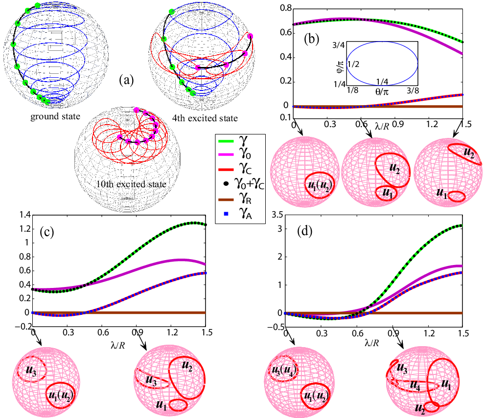
To illustrate the above theoretical results, we now consider an interacting boson system described by Hamiltonian $H=\frac{R\sin\theta}{4}\left(e^{i\varphi}\hat{a}^{{\dagger}}\hat{b}+e^{-i\varphi}\hat{b}^{{\dagger}}\hat{a}\right)+\frac{R\cos\theta}{2}\left(\hat{a}^{{\dagger}}\hat{a}-\hat{b}^{{\dagger}}\hat{b}\right)+\frac{\lambda}{4}\left(\hat{a}^{{\dagger}}\hat{a}-\hat{b}^{{\dagger}}\hat{b}\right)^{2}$, where $R\cos\theta$ is the energy offset between the two modes. The parameter $R\sin\theta e^{i\varphi}$ measures the coupling between the two modes, and $\lambda=g/V$ with $g$ being the interaction strength between bosons and $V$ being the volume of the system. This model equals to a spin system[20] and can be derived from the bosonic-field Hamiltonian[27] and has received extraordinary attention in the literature on BECs[28]. We numerically calculate the parameter dependent eigenstates of the $H$. Then, we use the formula (to avoid errors from numerical differential, see Ref.[12]) $e^{i\gamma}=\langle\psi|\psi^{\prime}\rangle\langle\psi^{\prime}|\psi^{\prime\prime}\rangle\cdots\langle\psi^{{}^{\prime}\cdots^{\prime}}|\psi\rangle$ to calculate the Berry phase $\gamma$, and compare it with the numerical result of Eq. (4) in which the time evolutions of majorana stars are obtained by solving the the roots of the equation (3) for corresponding eigenstate numerically.

For $\lambda=0$, the Hamiltonian $H$ reduces to the one of spin-$n/2$ in a magnetic field $\bm{B}=\frac{R}{2}(\sin\theta\cos\varphi,\sin\theta\cos\varphi,\cos\theta)$ as in case (ii) above. Therefore, for the $m$th eigenstate, we have $\gamma=(n-2m)\Omega_{\bm{u}}$, for example $2\Omega_{\bm{u}_{1}}$ for ground state of $H$ with two bosons in Fig. 2 (b), $\Omega_{\bm{u}_{1}}$ for first excited state of three bosons in Fig. 2 (c), and $0$ for second excited state of four bosons in Fig. 2 (d), respectively.

As the interacting constant $\lambda$ increase, the interaction between the bosons breaks the coincidences of stars. Note that our system can be mapped onto a spin system described by the LMG model similar to Ref.[20], the stars for the instantaneous eigenstate of $H$ are thus spread over two curves on the Bloch sphere. Its $m$th eigenstate has $n+1-m$ stars on one curve and $m-1$ stars on the other curve[20], such as the ground state, $4$th excited state and $10$th excited state for ten bosons shown in Fig. 2(a). As the adiabatic parameters evolve, the trajectories of stars become several different loops and the correlation phases arise. As Fig. 2 shows, the phase $\gamma_{R}^{(n)}$ vanish due to the symmetry between the stars on the two curves. And the Berry phase $\gamma$, calculated directly by its original definition, perfectly matches with $\gamma_{0}+\gamma_{C}$ in our theory.

Besides, we can use these changes of the symmetry of the states to clarify the type of state. e.g. the states of two bosons with coincident stars or separated stars (see the spheres in Fig. 2(b)); The states of three bosons with three coincident stars, two coincident stars or three separated stars (see the spheres in Fig. 2(c)). This clarification is according to the correlation between stars and may be related with entanglement.

In particular, the spin-$J$ state in Eq. (1) is equal to a symmetric $2J$-qubit pure state. By studying the entanglement of these symmetric qubit pure states, the entanglement of two and three qubits are found to be determined by the distance $d_{ij}$. For $n=2$, the concurrence[29] equals to $\mathcal{C}=d_{12}/2N_{1}^{2}$. Therefore, the correlation phase of the state is directly related to its entanglement: $\gamma_{C}^{(2)}=\frac{1}{2}\oint\mathcal{C}\Omega(\mathrm{d}\bm{u}_{12})$. For $n=3$, there exist different measurements for three different entanglement classes[30, 19] of states: the concurrence for the W type[31] of states becomes $\mathcal{C}_{12}=\frac{2d_{12}}{3N_{3}^{2}}$, where two of the three stars coincide with each other, and the correlation phase of the W type state can be written in the form of concurrence like two qubits: $\gamma_{C}^{(3)}=\frac{3}{2}\oint\Omega(\mathrm{d}\bm{u}_{12})\mathcal{C}_{12}$; the $3$-tangle[32] for the Greenberg-Horne-Zeilinger (GHZ)[33] type of states can be written as $\tau=\frac{2}{3}\beta_{12}\beta_{13}\beta_{23}N_{3}^{2}$ with three unequal stars; the three same stars at one point bring no entanglement and thus no correlation phase for the separable states. This means that the types of entanglement can be distinguished by the number of unequal stars (or diversity degree of the state[19]), and measured by a normalized product of the distance between unequal stars. Since the classification of entanglement by the number of unequal stars also hold for $n$ qubits ([19]), such as separable type ($n_{s}=1$), W type ($n_{s}=2$), and GHZ type ($n_{s}=n$), the normalized product of distances between unequal stars $(\prod_{\begin{smallmatrix}i,j=1\\ i<j\end{smallmatrix}}^{n_{s}}d_{ij})/N_{n}^{2(n_{s}-1)}$ may be a valid measure of entanglement. Besides, there are some other points for MSR worth further studying, such as identical particles in MSR and stars with permuted ends, we will address all these issues in a future paper.

The Majorana’s stellar representation and recently relevant applications have indicated that the evolution of a high spin state can be displayed intuitively by loops of MSs on the Bloch sphere. Our study here is to show how can we “read out” the physical effects of the state such as Berry phase and entanglement from these stars and loops. The discussion shows that the Berry phase of a spin-$J$ state is not only determined by the solid angles subtended by every Majorana star’s evolution path but also associated with the correlation between the stars. However, if we treat the MSR as a parameterizing process, MSR can be used for any states in a Hilbert space of arbitrary dimensions. For a $n$-dimensional generic state $|\psi\rangle^{n}=\sum_{m=1}^{n}C_{m}|m\rangle$, we can still use the roots $y_{i}=\tan\frac{\theta^{\prime}_{i}}{2}e^{i\phi^{\prime}_{i}}$ of equation $\sum_{l=0}^{n-1}[(-1)^{l}C_{n-l}y^{n-1-l}]/(\sqrt{(n-1-l)!l!})=0$ to define $n-1$ Majorana stars $u_{i}(\theta^{\prime}_{i},\phi^{\prime}_{i})$. These stars can also represent state $|\psi\rangle^{n}$ accordingly. Since, the Berry phase is decided by the parameter-dependent probability amplitudes $C_{m}$ with unchanged basis $|m\rangle$, and the basis $|m\rangle$ of dimension $n$ can be mapped to the basis of state for a spin-$(n-1)/2$ system. The Berry phase for $|\psi\rangle^{n}$ will take the same form as Eq. (3). Therefore, our results for Berry phase actually hold for any finite quantum system, and can be widely applied in various fields.

We thank B. Wu and H. Zhai for helpful discussions. This work is supported by the National Basic Research Program of China (973 Program) (Grants No. 2013CBA01502, No. 2011CB921503, and No. 2013CB834100), the National Natural Science Foundation of China (Grants No. 11374040, No. 11274051, and No. 11405008).

References

- [1] B. Simon, Phys. Rev. Lett. 51, 2167 (1983)
- [2] D. Chruściński, and A. Jamiołkowski, Geometric Phases in Classical and Quantum Mechanics (Birkhäuser, Berlin, 2004).
- [3] A. Bohm, A. Mostafazadeh, H.Koizumi, Q. Niu, and J. Zwanziger, The Geometric Phase in Quantum Systems (Springer-Verlag, Berlin, 2003).
- [4] M. V. Berry, Proc. R. Soc. A 392, 45 (1984).
- [5] Di Xiao, Ming-Che Zhang, and Qian Niu, Rev. Mod. Phys. 82, 1959 (2010).
- [6] N. Nagaosa, J. Sinova, S. Onoda, A. H. MacDonald, and N. P. Ong, Rev. Mod. Phys. 82, 1539 (2010).
- [7] R. D. King-Smith and D. Vanderbilt, Phys. Rev. B 47, 1651 (1993).
- [8] S. Xu, Y. Xia, L. Wray, S. Jia, and F. Meier, Science 332, 560 (2011).
- [9] J. C. Loredo, M. A. Broome, D. H. Smith, and A. G. White, Phys. Rev. Lett. 112, 143603 (2014).
- [10] E. Majorana, Nuovo Cimento 9, 43 (1932).
- [11] J. Schwinger, in Quantum Theory of Angular Momentum, edited by L. C. Biendenharn and H. Van Dam (Academic Press, New York, 1965).
- [12] J. H. Hannay, J. Phys. A 31, 520, 253 (1998).
- [13] Y. Kawaguchi and M. Ueda, Phys. Rep. (2012).
- [14] D. Stamper-Kurn and M. Ueda, Rev. Mod. Phys. 85, 1191 (2013).
- [15] B. Lian, T. L. Ho, and H. Zhai, Phys. Rev. A 85, 051606(R) (2012).
- [16] X. L. Cui, B. Lian, T. L. Ho, B. L. Lev, and H. Zhai, Phys. Rev. A, 88, 011601(R) (2013).
- [17] P. Bruno, Phys. Rev. Lett. 108, 240402 (2012).
- [18] Q. Niu, Physics 5, 65 (2012).
- [19] T. Bastin, S. Krins, P. Mathonet, M. Godefroid, L. Lamata, and E. Solano, Phys. Rev. Lett. 103, 070503 (2009).
- [20] P. Ribeiro, J. Vidal, and R. Mosseri, Phys. Rev. Lett. 99, 050402 (2007); P. Ribeiro, J. Vidal, and R. Mosseri, Phys. Rev. E 78, 021106 (2008).
- [21] E. Cornell and C. Wieman, Rev. Mod. Phys. 74, 875 (2002).
- [22] C. J. Myatt, E. A. Burt, R. W. Ghrist, E. A. Cornell, and C. E. Wieman Phys. Rev. Lett. 78, 586 (1997).
- [23] See Supplemental Material for derivations of the normalization coefficient , the Berry phase , and the solid angle in Eq. (7).
- [24] C. Lee, J. Phys. A 21, 3749 (1988).
- [25] W. Ganczarek, M. Kuś, and K. Życzkowski, Phys. Rev. A 85, 032314 (2012).
- [26] M. V. Berry, in Anomalies, Phases, Defects, edited by U. M. Bregola, G. Marmo, and G. Morandi (Bibliopolis, Naples, 1990).
- [27] J. I. Cirac, M. Lewenstein, K. Mølmer, and P. Zoller, Phys. Rev. A 57, 1208 (1998).
- [28] A. Leggett, Rev. Mod. Phys. 73, 307 (2001); B. Wu, Q. Zhang, and J. Liu, Phys. Lett. A 375, 545 (2011); S. C. Li, J. Liu, and L. B. Fu, Phys. Rev. A 83, 042107 (2011).
- [29] W. K. Wootters, Phys. Rev. Lett. 80, 2245 (1998).
- [30] A. Acín, D. Bruß, M. Lewenstein, and A. Sanpera, Phys. Rev. Lett. 87, 040401 (2001).
- [31] W. Dür, G. Vidal, and J. I. Cirac, Phys. Rev. A 62, 062314 (2000).
- [32] V. Coffman, J. Kundu, and W. K. Wootters, Phys. Rev. A 61, 052306 (2000).
- [33] D. M. Greenberger, M. Horne, and A. Zeilinger, Bell’s Theorem, Quantum Theory, and Conceptions of the Universe, edited by M. Kafatos (Kluwer, Dordrecht, 1989).