On the Convergence Rate of Decomposable Submodular Function Minimization
Abstract
Submodular functions describe a variety of discrete problems in machine learning, signal processing, and computer vision. However, minimizing submodular functions poses a number of algorithmic challenges. Recent work introduced an easy-to-use, parallelizable algorithm for minimizing submodular functions that decompose as the sum of “simple” submodular functions. Empirically, this algorithm performs extremely well, but no theoretical analysis was given. In this paper, we show that the algorithm converges linearly, and we provide upper and lower bounds on the rate of convergence. Our proof relies on the geometry of submodular polyhedra and draws on results from spectral graph theory.
1 Introduction
A large body of recent work demonstrates that many discrete problems in machine learning can be phrased as the optimization of a submodular set function [2]. A set function over a ground set of elements is submodular if the inequality holds for all subsets . Problems like clustering [33], structured sparse variable selection [1], MAP inference with higher-order potentials [28], and corpus extraction problems [31] can be reduced to the problem of submodular function minimization (SFM), that is
| (P1) |
Although SFM is solvable in polynomial time, existing algorithms can be inefficient on large-scale problems. For this reason, the development of scalable, parallelizable algorithms has been an active area of research [24, 25, 29, 35]. Approaches to solving Problem (P1) are either based on combinatorial optimization or on convex optimization via the Lovász extension.
Functions that occur in practice are usually not arbitrary and frequently possess additional exploitable structure. For example, a number of submodular functions admit specialized algorithms that solve Problem (P1) very quickly. Examples include cut functions on certain kinds of graphs, concave functions of the cardinality , and functions counting joint ancestors in trees. We will use the term simple to refer to functions for which we have a fast subroutine for minimizing , where is any modular function. We treat these subroutines as black boxes. Many commonly occuring submodular functions (for example, graph cuts, hypergraph cuts, MAP inference with higher-order potentials [16, 28, 37], co-segmentation [22], certain structured-sparsity inducing functions [26], covering functions [35], and combinations thereof) can be expressed as a sum
| (1) |
of simple submodular functions. Recent work demonstrates that this structure offers important practical benefits [25, 29, 35]. For instance, it admits iterative algorithms that minimize each separately and combine the results in a straightforward manner (for example, dual decomposition).
In particular, it has been shown that the minimization of decomposable functions can be rephrased as a best-approximation problem, the problem of finding the closest points in two convex sets [25]. This formulation brings together SFM and classical projection methods and yields empirically fast, parallel, and easy-to-implement algorithms. In these cases, the performance of projection methods depends heavily on the specific geometry of the problem at hand and is not well understood in general. Indeed, while Jegelka et al. [25] show good empirical results, the analysis of this alternative approach to SFM was left as an open problem.
Contributions. In this work, we study the geometry of the submodular best-approximation problem and ground the prior empirical results in theoretical guarantees. We show that SFM via alternating projections, or block coordinate descent, converges at a linear rate. We show that this rate holds for the best-approximation problem, relaxations of SFM, and the original discrete problem. More importantly, we prove upper and lower bounds on the worst-case rate of convergence. Our proof relies on analyzing angles between the polyhedra associated with submodular functions and draws on results from spectral graph theory. It offers insight into the geometry of submodular polyhedra that may be beneficial beyond the analysis of projection algorithms.
Submodular minimization. The first polynomial-time algorithm for minimizing arbitrary submodular functions was a consequence of the ellipsoid method [19]. Strongly and weakly polynomial-time combinatorial algorithms followed [32]. The current fastest running times are [34] in general and for integer-valued functions [23], where and is the time required to evaluate . Some work has addressed decomposable functions [25, 29, 35]. The running times in [29] apply to integer-valued functions and range from for cuts to , where is the maximal cardinality of the support of any , and is the time required to minimize a simple function. Stobbe and Krause [35] use a convex optimization approach based on Nesterov’s smoothing technique. They achieve a (sublinear) convergence rate of for the discrete SFM problem. Their results and our results do not rely on the function being integral.
Projection methods. Algorithms based on alternating projections between convex sets (and related methods such as the Douglas–Rachford algorithm) have been studied extensively for solving convex feasibility and best-approximation problems [4, 5, 7, 11, 12, 20, 21, 36, 38]. See Deutsch [10] for a survey of applications. In the simple case of subspaces, the convergence of alternating projections has been characterized in terms of the Friedrichs angle between the subspaces [5, 6]. There are often good ways to compute (see Lemma 6), which allow us to obtain concrete linear rates of convergence for subspaces. The general case of alternating projections between arbitrary convex sets is less well understood. Bauschke and Borwein [3] give a general condition for the linear convergence of alternating projections in terms of the value (defined in Section 3.1). However, except in very limited cases, it is unclear how to compute or even bound . While it is known that for polyhedra [5, Corollary 5.26], the rate may be arbitrarily slow, and the challenge is to bound the linear rate away from one. We are able to give a specific uniform linear rate for the submodular polyhedra that arise in SFM.
Although both and are useful quantities for understanding the convergence of projection methods, they largely have been studied independently of one another. In this work, we relate these two quantities for polyhedra, thereby obtaining some of the generality of along with the computability of . To our knowledge, we are the first to relate and outside the case of subspaces. We feel that this connection may be useful beyond the context of submodular polyhedra.
1.1 Background
Throughout this paper, we assume that is a sum of simple submodular functions and that . Points can be identified with (modular) set functions via . The base polytope of is defined as the set of all modular functions that are dominated by and that sum to ,
The Lovász extension of can be written as the support function of the base polytope, that is . Even though may have exponentially many faces, the extension can be evaluated in time [15]. The discrete SFM problem (P1) can be relaxed to the non-smooth convex optimization problem
| (P2) |
where is the Lovász extension of . This relaxation is exact – rounding an optimal continuous solution yields the indicator vector of an optimal discrete solution. The formulation in Problem (P2) is amenable to dual decomposition [30] and smoothing techniques [35], but suffers from the non-smoothness of [25]. Alternatively, we can formulate a proximal version of the problem
| (P3) |
By thresholding the optimal solution of Problem (P3) at zero, we recover the indicator vector of an optimal discrete solution [17], [2, Proposition 8.4].
Lemma 1.
Lemma 1 implies that we can minimize a decomposable submodular function by solving Problem (P4), which means finding the closest points between the subspace and the product of base polytopes. Projecting onto is straightforward because is a subspace. Projecting onto amounts to projecting onto each separately. The projection of a point onto may be solved by minimizing [25]. We can compute these projections easily because each is simple.
Throughout this paper, we use and to refer to the specific polyhedra defined in Lemma 1 (which live in ) and and to refer to general polyhedra (sometimes arbitrary convex sets) in . Note that the polyhedron depends on the submodular functions , but we omit the dependence to simplify our notation. Our bound will be uniform over all submodular functions.
2 Algorithm and Idea of Analysis
A popular class of algorithms for solving best-approximation problems are projection methods [5]. The most straightforward approach uses alternating projections (AP) or block coordinate descent. Start with any point , and inductively generate two sequences via and . Given the nature of and , this algorithm is easy to implement and use in our setting, and it solves Problem (P4) [25]. This is the algorithm that we will analyze.
The sequence will eventually converge to an optimal pair . We say that AP converges linearly with rate if and for all and for some constants and . Smaller values of are better.
Analysis: Intuition. We will provide a detailed analysis of the convergence of AP for the polyhedra and . To motivate our approach, we first provide some intuition with the following much-simplified setup. Let and be one-dimensional subspaces spanned by the unit vectors and respectively. In this case, it is known that AP converges linearly with rate , where is the angle such that . The smaller the angle, the slower the rate of convergence. For subspaces and of higher dimension, the relevant generalization of the “angle” between the subspaces is the Friedrichs angle [11, Definition 9.4], whose cosine is given by
| (2) |
In finite dimensions, . In general, when and are subspaces of arbitrary dimension, AP will converge linearly with rate [11, Theorem 9.8]. If and are affine spaces, AP still converges linearly with rate , where and .
We are interested in rates for polyhedra and , which we define as the intersection of finitely many halfspaces. We generalize the preceding results by considering all pairs of faces of and and showing that the convergence rate of AP between and is at worst , where is the affine hull of and for some . The faces of are defined as the nonempty maximizers of linear functions over , that is
| (3) |
While we look at angles between pairs of faces, we remark that Deutsch and Hundal [13] consider a different generalization of the “angle” between arbitrary convex sets.
Roadmap of the Analysis. Our analysis has two main parts. First, we relate the convergence rate of AP between polyhedra and to the angles between the faces of and . To do so, we give a general condition under which AP converges linearly (Theorem 2), which we show depends on the angles between the faces of and (Corollary 5) in the polyhedral case. Second, we specialize to the polyhedra and , and we equate the angles with eigenvalues of certain matrices and use tools from spectral graph theory to bound the relevant eigenvalues in terms of the conductance of a specific graph. This yields a worst-case bound of on the rate, stated in Theorem 12.
In Theorem 14, we show a lower bound of on the worst-case convergence rate.
3 The Upper Bound
We first derive an upper bound on the rate of convergence of AP between the polyhedra and . The results in this section are proved in Appendix A.
3.1 A Condition for Linear Convergence
We begin with a condition under which AP between two closed convex sets and converges linearly. This result is similar to that of Bauschke and Borwein [3, Corollary 3.14], but the rate we achieve is twice as fast and relies on slightly weaker assumptions.
We will need a few definitions from Bauschke and Borwein [3]. Let be the distance between sets and . Define the sets of “closest points” as
| (4) |
and let (see Figure 1). Note that , and when we have and . Therefore, we can think of the pair as a generalization of the intersection to the setting where and do not intersect. Pairs of points are solutions to the best-approximation problem between and . In our analysis, we will mostly study the translated version of that intersects at .
For , the function relates the distance to with the distances to and ,
If is bounded, then whenever is close to both and , it must also be close to their intersection. If, for example, and and are balls of radius one whose centers are separated by distance exactly two, then is unbounded. The maximum is useful for bounding the convergence rate.
Theorem 2.
Let and be convex sets, and suppose that . Then AP between and converges linearly with rate . Specifically,
3.2 Relating to the Angles Between Faces of the Polyhedra
In this section, we consider the case of polyhedra and , and we bound in terms of the angles between pairs of their faces. In Lemma 3, we show that is nondecreasing along the sequence of points generated by AP between and . We treat points for which separately because those are the points from which AP between and converges in one step. This lemma enables us to bound by initializing AP at and bounding at some later point in the resulting sequence.
Lemma 3.
For any , either or . Similarly, for any , either or .
We can now bound by angles between faces of and .
Proposition 4.
If and are polyhedra and , then there exist faces and such that
The analogous statement holds when we replace with .
Note that . Proposition 4 immediately gives us the following corollary.
Corollary 5.
If and are polyhedra, then
3.3 Angles Between Subspaces and Singular Values
Corollary 5 leaves us with the task of bounding the Friedrichs angle. To do so, we first relate the Friedrichs angle to the singular values of certain matrices in Lemma 6. We then specialize this to base polyhedra of submodular functions. For convenience, we prove Lemma 6 in Appendix A.5, though this result is implicit in the characterization of principal angles between subspaces given in [27, Section 1]. Ideas connecting angles between subspaces and eigenvalues are also used by Diaconis et al. [14].
Lemma 6.
Let and be matrices with orthonormal rows and with equal numbers of columns. If all of the singular values of equal one, then . Otherwise, is equal to the largest singular value of that is less than one.
Faces of relevant polyhedra. Let and be faces of the polyhedra and from Lemma 1. Since is a vector space, its only nonempty face is . Hence, , where is an matrix of identity matrices :
| (5) |
The matrix for requires a bit more elaboration. Since is a Cartesian product, we have , where and is a face of . To proceed, we use the following characterization of faces of base polytopes [2, Proposition 4.7].
Proposition 7.
Let be a submodular function, and let be a face of . Then there exists a partition of into disjoint sets such that
The following corollary is immediate.
Corollary 8.
Define , , and as in Proposition 7. Then
By Corollary 8, for each , there exists a partition of into disjoint sets such that
| (6) |
In other words, we can write as the nullspace of either of the matrices
where is the indicator vector of . For , this follows directly from Equation (6). can be obtained from via left multiplication by an invertible matrix, so and have the same nullspace. Lemma 6 then implies that equals the largest singular value of
that is less than one. We rephrase this conclusion in the following remark.
Remark 9.
The largest eigenvalue of less than one equals .
Let . Then is the square matrix whose rows and columns are indexed by with and and whose entry corresponding to row and column equals
3.4 Bounding the Relevant Eigenvalues
It remains to bound the largest eigenvalue of that is less than one. To do so, we view the matrix in terms of the symmetric normalized Laplacian of a weighted graph. Let be the graph whose vertices are indexed by with and . Let the edge between vertices and have weight . We may assume that is connected (the analysis in this case subsumes the analysis in the general case). The symmetric normalized Laplacian of this graph is closely related to our matrix of interest,
| (7) |
Hence, the largest eigenvalue of that is less than one can be determined from the smallest nonzero eigenvalue of . We bound via Cheeger’s inequality (stated in Appendix A.6) by bounding the Cheeger constant of .
Lemma 10.
For , we have and hence .
We prove Lemma 10 in Appendix A.7. Combining Remark 9, Equation (7), and Lemma 10, we obtain the following bound on the Friedrichs angle.
Proposition 11.
Assuming that , we have
Theorem 12.
The AP algorithm for Problem (P4) converges linearly with rate , i.e.,
4 A Lower Bound
To probe the tightness of Theorem 12, we construct a “bad” submodular function and decomposition that lead to a slow rate. Appendix B gives the formal details. Our example is an augmented cut function on a cycle: for each , define to be the cut function of a single edge ,
Take to be even and and define the submodular function , where
and for all . The optimal solution to the best-approximation problem is the all zeros vector.
Lemma 13.
The cosine of the Friedrichs angle between and is
Around the optimal solution , the polyhedra and behave like subspaces, and it is possible to pick initializations and such that the Friedrichs angle exactly determines the rate of convergence. That means , and
Bounding leads to the following lower bound on the rate.
Theorem 14.
There exists a decomposed function and initializations for which the convergence rate of AP is at least .
5 Convergence of the Primal Objective
We have shown that AP generates a sequence of points and in such that linearly, where minimizes the objective in Problem (P4). In this section, we show that this result also implies the linear convergence of the objective in Problem (P3) and of the original discrete objective in Problem (P1). The proofs may be found in Appendix C.
Define the matrix , where is the matrix defined in Equation (5). Multiplication by maps a vector to , where for each . Set and . As shown in Jegelka et al. [25], Problem (P3) is minimized by .
Proposition 15.
We have linearly with rate .
This linear rate of convergence translates into a linear rate for the original discrete problem.
Theorem 16.
Choose . Let be the suplevel set of with smallest value of . Then linearly with rate .
6 Discussion
In this work, we analyze projection methods for parallel SFM and give upper and lower bounds on the linear rate of convergence. This means that the number of iterations required for an accuracy of is logarithmic in , not linear as in previous work [35]. Our rate is uniform over all submodular functions. Moreover, our proof highlights how the number of components and the facial structure of affect the convergence rate. These insights may serve as guidelines when working with projection algorithms and aid in the analysis of special cases. For example, reducing is often possible. Any collection of that have disjoint support, such as the cut functions corresponding to the rows or columns of a grid graph, can be grouped together without making the projection harder.
Our analysis also shows the effects of additional properties of . For example, suppose that is separable, that is, for some nonempty . Then the subsets defining the relevant faces of satisfy either or [2]. This makes in Section 3.4 disconnected, and as a result, the in Theorem 12 gets replaced by for an improved rate. This applies without the user needing to know when running the algorithm.
A number of future directions suggest themselves. For example, Jegelka et al. [25] also considered the related Douglas–Rachford (DR) algorithm. DR between subspaces converges linearly with rate [6], as opposed to for AP. We suspect that our approach may be modified to analyze DR between polyhedra. Further questions include the extension to cyclic updates (instead of parallel ones), multiple polyhedra, and stochastic algorithms.
Acknowledgments.
We would like to thank Mădălina Persu for suggesting the use of Cheeger’s inequality. This research is supported in part by NSF CISE Expeditions Award CCF-1139158, LBNL Award 7076018, and DARPA XData Award FA8750-12-2-0331, and gifts from Amazon Web Services, Google, SAP, The Thomas and Stacey Siebel Foundation, Apple, C3Energy, Cisco, Cloudera, EMC, Ericsson, Facebook, GameOnTalis, Guavus, HP, Huawei, Intel, Microsoft, NetApp, Pivotal, Splunk, Virdata, VMware, WANdisco, and Yahoo!. This work is supported in part by the Office of Naval Research under grant number N00014-11-1-0688, the US ARL and the US ARO under grant number W911NF-11-1-0391, and the NSF under grant number DGE-1106400.
References
- [1] F. Bach. Structured sparsity-inducing norms through submodular functions. In Advances in Neural Information Processing Systems, 2011.
- [2] F. Bach. Learning with submodular functions: A convex optimization perspective. Foundations and Trends in Machine Learning, 6(2-3):145–373, 2013.
- [3] H. H. Bauschke and J. M. Borwein. On the convergence of von Neumann’s alternating projection algorithm for two sets. Set-Valued Analysis, 1(2):185–212, 1993.
- [4] H. H. Bauschke and J. M. Borwein. Dykstra’s alternating projection algorithm for two sets. Journal of Approximation Theory, 79(3):418–443, 1994.
- [5] H. H. Bauschke and J. M. Borwein. On projection algorithms for solving convex feasibility problems. SIAM Review, 38(3):367–426, 1996.
- [6] H. H. Bauschke, J. B. Cruz, T. T. Nghia, H. M. Phan, and X. Wang. The rate of linear convergence of the Douglas–Rachford algorithm for subspaces is the cosine of the Friedrichs angle. Journal of Approximation Theory, 185:63–79, 2014.
- [7] A. Beck and L. Tetruashvili. On the convergence of block coordinate descent type methods. SIAM Journal on Optimization, 23(4):2037–2060, 2013.
- [8] J. V. Burke and J. J. Moré. On the identification of active constraints. SIAM Journal on Numerical Analysis, 25(5):1197–1211, 1988.
- [9] F. R. Chung. Spectral Graph Theory. American Mathematical Society, 1997.
- [10] F. Deutsch. The method of alternating orthogonal projections. In Approximation Theory, Spline Functions and Applications, pages 105–121. Springer, 1992.
- [11] F. Deutsch. Best Approximation in Inner Product Spaces, volume 7. Springer, 2001.
- [12] F. Deutsch and H. Hundal. The rate of convergence of Dykstra’s cyclic projections algorithm: The polyhedral case. Numerical Functional Analysis and Optimization, 15(5-6):537–565, 1994.
- [13] F. Deutsch and H. Hundal. The rate of convergence for the cyclic projections algorithm I: angles between convex sets. Journal of Approximation Theory, 142(1):36–55, 2006.
- [14] P. Diaconis, K. Khare, and L. Saloff-Coste. Stochastic alternating projections. Illinois Journal of Mathematics, 54(3):963–979, 2010.
- [15] J. Edmonds. Combinatorial Structures and Their Applications, chapter Submodular Functions, Matroids and Certain Polyhedra, pages 69–87. Gordon and Breach, 1970.
- [16] A. Fix, T. Joachims, S. Park, and R. Zabih. Structured learning of sum-of-submodular higher order energy functions. In Int. Conference on Computer Vision (ICCV), 2013.
- [17] S. Fujishige and S. Isotani. A submodular function minimization algorithm based on the minimum-norm base. Pacific Journal of Optimization, 7:3–17, 2011.
- [18] R. M. Gray. Toeplitz and circulant matrices: A review. Foundations and Trends in Communications and Information Theory, 2(3):155–239, 2006.
- [19] M. Grötschel, L. Lovász, and A. Schrijver. The ellipsoid method and its consequences in combinatorial optimization. Combinatorica, 1(2):169–197, 1981.
- [20] L. Gubin, B. Polyak, and E. Raik. The method of projections for finding the common point of convex sets. USSR Computational Mathematics and Mathematical Physics, 7(6):1–24, 1967.
- [21] I. Halperin. The product of projection operators. Acta Sci. Math. (Szeged), 23:96–99, 1962.
- [22] D. Hochbaum and V. Singh. An efficient algorithm for co-segmentation. In Int. Conference on Computer Vision (ICCV), 2009.
- [23] S. Iwata. A faster scaling algorithm for minimizing submodular functions. SIAM J. on Computing, 32:833–840, 2003.
- [24] S. Jegelka, H. Lin, and J. Bilmes. On fast approximate sumodular minimization. In Advances in Neural Information Processing Systems, 2011.
- [25] S. Jegelka, F. Bach, and S. Sra. Reflection methods for user-friendly submodular optimization. In Advances in Neural Information Processing Systems, pages 1313–1321, 2013.
- [26] R. Jenatton, J. Mairal, G. Obozinski, and F. Bach. Proximal methods for hierarchical sparse coding. JMLR, page 2297–2334, 2011.
- [27] A. V. Knyazev and M. E. Argentati. Principal angles between subspaces in an A-based scalar product: algorithms and perturbation estimates. SIAM Journal on Scientific Computing, 23(6):2008–2040, 2002.
- [28] P. Kohli, L. Ladický, and P. Torr. Robust higher order potentials for enforcing label consistency. Int. Journal of Computer Vision, 82, 2009.
- [29] V. Kolmogorov. Minimizing a sum of submodular functions. Discrete Applied Mathematics, 160(15):2246–2258, 2012.
- [30] N. Komodakis, N. Paragios, and G. Tziritas. MRF energy minimization and beyond via dual decomposition. IEEE Trans. Pattern Analysis and Machine Intelligence, 2011.
- [31] H. Lin and J. Bilmes. Optimal selection of limited vocabulary speech corpora. In Proc. Interspeech, 2011.
- [32] S. McCormick. Handbook on Discrete Optimization, chapter Submodular Function Minimization, pages 321–391. Elsevier, 2006.
- [33] M. Narasimhan and J. Bilmes. Local search for balanced submodular clusterings. In IJCAI, pages 981–986, 2007.
- [34] J. Orlin. A faster strongly polynomial time algorithm for submodular function minimization. Math. Programming, 118:237–251, 2009.
- [35] P. Stobbe and A. Krause. Efficient minimization of decomposable submodular functions. In Advances in Neural Information Processing Systems, 2010.
- [36] P. Tseng. Alternating projection-proximal methods for convex programming and variational inequalities. SIAM Journal on Optimization, 7(4):951–965, 1997.
- [37] S. Vicente, V. Kolmogorov, and C. Rother. Joint optimization of segmentation and appearance models. In Int. Conference on Computer Vision (ICCV), 2009.
- [38] J. Von Neumann. Functional Operators: The Geometry of Orthogonal Spaces. Princeton University Press, 1950.
Appendix A Upper Bound Results
A.1 Proof of Theorem 2
For the proof of this theorem, we will need the fact that projection maps are firmly nonexpansive, that is, for a closed convex nonempty subset , we have
for all . Now, suppose that . Let and note that and that . We have
It follows that . Similarly, we have . When combining these, induction shows that
As shown in [3, Theorem 3.3], the above implies that and and that
A.2 Connection Between and in the Subspace Case
In this section, we introduce a simple lemma connecting and in the case of subspaces and . We will use this lemma in several subsequent proofs.
Lemma 17.
Let and be subspaces and suppose and that . Then
- (a)
- (b)
- (c)
if and only if .
A.3 Proof of Lemma 3
It suffices to prove the statement for . For , define , , and , where denotes the line segment between and (which is contained in by convexity). See Figure 2 for a graphical depiction. If , then . So we may assume that which also implies that and . We have
| (8) |
The first inequality holds because and . The middle inequality holds because the area of the triangle with vertices , , and can be expressed as both and , where is the angle between vectors and , so
The third inequality holds because and . The chain of inequalities in Equation (8) prove the lemma.
A.4 Proof of Proposition 4
Suppose that (the case is the same), and let . If , the statement is evident, so we may assume that . We will construct sequences of polyhedra
.
where is a face of and is a face of for . Either or will hold. We will further define , which will contain , so that we can define
for (this is just the function defined for the polyhedra and ). Our construction will yield points , and such that , , and for each . Furthermore, we will have
| (9) |
Now we describe the construction. For any , define to be the point obtained by moving by the appropriate amount toward . Note that is a nondecreasing function on the interval . Choose sufficiently small so that every face of either or that intersects , the ball of radius centered on , necessarily contains . Now choose sufficiently close to so that . It follows that is contained in the face of whose relative interior contains . It further follows that is contained in the face of whose relative interior contains because
To initialize the construction, set
and let and be the unique faces of and respectively such that and (the relative interiors of the faces of a polyhedron partition that polyhedron [8, Theorem 2.2]). Note that because . Note that so that
Now, inductively assume that we have defined , , , and satisfying the stated properties. Generate the sequences and with and by running AP between the polyhedra and initialized with . There are two possibilities, either and for every , or there is some for which either or . Note that and intersect and that AP between them will not terminate after a finite number of steps.
Suppose that and for every . Then set and terminate the procedure. Otherwise, choose such that either or . Now set and . Let and be the unique faces of and respectively such that and . Note that and . We have
The preceding work shows the inductive step. Note that if then and if then . One of these will hold, so the induction will terminate after a finite number of steps.
We have produced the sequence in Equation (9) and we have created , , and such that AP between and , when initialized at , generates the same sequence of points as AP between and . Using this fact, along with [12, Theorem 9.3], we see that . Using this, along with Lemma 17(b), we see that
| (10) |
Equations (10) and (9) prove the result. Note that and are faces of and respectively. We can switch between faces of and faces of because doing so amounts to translating by which does not affect the angles.
A.5 Proof of Lemma 6
We have
where the first equality uses the fact that for matrices , and the second equality uses the fact that for subspaces and [6, Fact 2.3].
Let and have dimensions and respectively, and let and be the subspaces spanned by the columns of and respectively. Without loss of generality, assume that . Let be the singular values of with corresponding left singular vectors and right singular vectors . Let and let for . By definition, we can write
Since the are orthonormal, so are the . Similarly, since the are orthonormal, so are the . Suppose that all of the singular values of equal one. Then we must have for each , which implies that , and so .
Now suppose that , and . It follows that
and so
A.6 Cheeger’s Inequality
For an overview of spectral graph theory, see Chung [9]. We state Cheeger’s inequality below.
Let be a weighted, connected graph with vertex set and edge weights . Define the weighted degree of a vertex to be , define the volume of a subset of vertices to be the sum of their weighted degrees, , and define the size of the cut between and its complement to be the sum of the weights of the edges between and ,
The Cheeger constant is defined as
Let be the unnormalized Laplacian of , i.e. the matrix whose entries are defined by
Let be the diagonal matrix defined by . Then is the normalized Laplacian. Let denote the second smallest eigenvalue of (since is connected, there will be exactly one eigenvalue equal to zero).
Theorem 18 (Cheeger’s inequality).
We have .
A.7 Proof of Lemma 10
Proof.
We have
Since is connected, for any nonempty set , there must be some element (here is the ground set of our submodular function , not the set of vertices ) such that for some and . Suppose that appears in of the subsets of indexed by elements of and in of the subsets of indexed by elements of . Then
It follows that
∎
It follows from Theorem 18 that .
Appendix B Results for the Lower Bound
B.1 Some Helpful Results
In Lemma 19, we show how AP between subspaces and can be initialized to exactly achieve the worst-case rate of convergence. Then in Corollary 20, we show that if subsets and look like subspaces and near the origin, we can initialize AP between and to achieve the same worst-case rate of convergence.
Lemma 19.
Let and be subspaces with and . Then there exists some nonzero point such that when we initialize AP at , the resulting sequences and satisfy
Proof.
Find and with and such that , which we can do by compactness. By Lemma 17(a),
Set and generate the sequences and via AP. Since , Lemma 17(c) implies that . Since attains its maximum at , Lemma 3 implies that attains the same value at every element of the sequences and . Therefore, Lemma 17(c) implies that and for all . This proves the lemma. ∎
Corollary 20.
Let and be subspaces with and . Let and be subsets such that and for some . Then there is a point such that the sequences and generated by AP between and initialized at satisfy
Proof.
Use Lemma 19 to choose some nonzero satisfying this property. Then set . ∎
B.2 Proof of Lemma 13
Observe that we can write
We can write as the nullspace of the matrix
where the identity matrix is repeated times and where and are the matrices
Recall that we can write as the nullspace of the matrix defined in Equation (5). It follows from Lemma 6 that equals the largest singular value of that is less than one. We have
We can permute the columns of without changing the singular values, so equals the largest singular value of
that is less than one, where is the circulant matrix
Therefore, equals the largest eigenvalue of
that is less than one. Therefore, it suffices to examine the circulant matrix
The eigenvalues of are given by for (see Gray [18, Section 3.1] for a derivation). Therefore,
B.3 Lower Bound Illustration
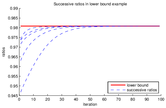
The proof of Theorem 14 shows that there is some such that when we initialize AP between and at , we generate a sequence satisfying
where is the optimal set. In Figure 3, we plot the theoretical bound in red, and in blue the successive ratios for five runs of AP between and with random initializations. Had we initialized AP at , the successive ratios would exactly equal . The plot of these ratios would coincide with the red line in Figure 3.
Figure 3 illustrates that the empirical behavior of AP between and is often similar to the worst-case behavior, even when the initialization is random. When we initialize AP randomly, the successive ratios appear to increase to the lower bound and then remain constant. Figure 3 shows the case and , but the plot looks similar for other and .
We also note that the graph corresponding to our lower bound example actually achieves a Cheeger constant similar to the one used in Lemma 10.
Appendix C Results for Convergence of the Primal and Discrete Problems
C.1 Proof of Proposition 15
First, suppose that . Let be the set of indices on which is nonnegative. Then we have
| (11) |
Recall that we defined . Now, we show that converges to linearly with rate . We will use Equation (11) to bound the norms of and , both of which lie in . We will also use the fact that . Finally, we will use the proof of Theorem 12 to bound . First, we bound the difference between the squared norms using convexity. We have
| (12) |
Next, we bound the difference in Lovász extensions. Choose . Then
| (13) |
Combining the bounds (12) and (13), we find that
| (14) |
C.2 Proof of Theorem 16
We will make use of the following result, shown in [2, Proposition 10.5] and stated below for convenience.
Proposition 21.
Let be a pair of primal-dual candidates for the minimization of , with duality gap . Then if is the suplevel set of with smallest value of , then
Using this result in our setting, recall that by definition is the set of the form for some constant with smallest value of .
Let be a primal-dual optimal pair for the left-hand version of Problem (P3). The dual of this minimization problem is the projection problem . From [2, Proposition 10.5], we see that
where the third inequality uses the proof of Proposition 15. The second inequality relies on Bach [2, Proposition 10.5], which states that a duality gap of for the left-hand version of Problem (P3) turns into a duality gap of for the original discrete problem. If our algorithm converged with rate , this would translate to a rate of for the discrete problem. But fortunately, our algorithm converges linearly, and taking a square root preserves linear convergence.
C.3 Running times
Theorem 16 implies that the number of iterations required for an accuracy of is at most
| (15) |
Each iteration involves minimizing each of the separately. For comparison, the number of iterations required in Stobbe and Krause [35] is
The dependence of this algorithm on and is better, but its dependence on is worse. For example, to obtain the exact discrete solution, we need . This is one for integer-valued functions (in which case the lower rate may be desirable), but can otherwise become very small. The constant can be of order in general (or even larger if the function becomes very negative). For empirical comparisons, we refer the reader to [25].
The running times of the combinatorial algorithm by Kolmogorov [29] apply to integer-valued functions (as opposed to the generic ones above) and range from for cuts to , where is the maximal cardinality of the support of any , and is the time required to minimize a simple function. This is better than (15) if is a small constant, and worse as gets closer to .
For comparison, if not exploiting decomposition, one may use combinatorial algorithms, the Frank-Wolfe algorithm (conditional gradient descent), or a subgradient method. The combinatorial algorithm by Orlin [34] has a running time of , and the algorithm by Iwata [23] (for integer-valued functions) has a running time of , where is the time required to evaluate . For an accuracy of in the discrete objective, Frank-Wolfe will take iterations, each taking time . The subgradient method behaves similarly.