Coherent versus measurement feedback:
Linear systems theory for quantum information

A standard form of classical linear systems is given by

$x(t)\in{\mathbb{R}}^{n}$ is a vector of $n$ c-number variables. $u(t)$ and $y(t)$ are vectors of real-valued input and output signals, respectively. $A,B$, and $C$ are real matrices with appropriate dimensions. In this paper, the following three questions are important; (i) which components of $x$ can be controlled by $u$, (ii) which components of $x$ can be observed from $y$, and (iii) in what condition $u$ does not appear in $y$? The answers are briefly described below. See [7, 8, 9] for more detailed discussion.

The first problem can be explicitly solved by examining the following controllability matrix:

Indeed this matrix fully characterizes the controllable and uncontrollable variables with respect to (w.r.t.) $u(t)$. To see this fact, suppose $m=\dim{\rm Range}({\cal C}_{u})<n$ and let $\{d_{i}^{(1)}\}$ and $\{d_{i}^{(2)}\}$ be independent vectors spanning ${\rm Range}({\cal C}_{u})$ and ${\rm Range}({\cal C}_{u})^{c}$, respectively. Further let us define $T_{1}=[d_{1}^{(1)},\ldots,d_{m}^{(1)}]$ and $T_{2}=[d_{1}^{(2)},\ldots,d_{n-m}^{(2)}]$. Then, as $A{\cal C}_{u}$ is spanned by $\{d_{i}^{(1)}\}$, there exists a matrix $A_{11}$ satisfying $AT_{1}=T_{1}A_{11}$. On the other hand $AT_{2}$ is in general spanned by all the vectors; i.e. $AT_{2}=T_{1}A_{12}+T_{2}A_{22}$. Note also that there exists a matrix $B_{1}$ satisfying $B=T_{1}B_{1}$. These relations are summarized in terms of the invertible square matrix $T=[T_{1},T_{2}]$ as

Thus the dynamics of $x^{\prime}=T^{-1}x$ is given by

Clearly $x^{\prime}_{2}=V_{2}^{\top}x$ is free from $u$, where $[V_{1},V_{2}]^{\top}=T^{-1}$; in particular, due to $V_{2}^{\top}T_{1}=0$, the uncontrollable variable $x^{\prime}_{2}$ is characterized by ${\rm Range}(V_{2})={\rm Ker}({\cal C}_{u}^{\top})$. Also the controllable one $x^{\prime}_{1}=V_{1}^{\top}x$ is defined in ${\rm Range}(V_{1})={\rm Ker}({\cal C}_{u}^{\top})^{c}$. Hence we call these sets the uncontrollable subspace and the controllable subspace, respectively ¹¹ 1 Usually the controllable and uncontrollable subspaces are defined by ${\rm Range}({\cal C}_{u})$ and ${\rm Range}({\cal C}_{u})^{c}$, respectively. But in the quantum case a variable of interest is an infinite-dimensional operator and does not live in either of these subspaces; rather it is always of the form $v^{\top}\hat{x}$ and thus can be well characterized by the dual vector $v\in{\mathbb{R}}^{2n}$. This is the reason why we define the controllable and uncontrollable subspaces in the dual space as ${\rm Ker}({\cal C}_{u}^{\top})^{c}$ and ${\rm Ker}({\cal C}_{u}^{\top})$, respectively. . The following fact is especially useful in this paper: the system has an uncontrollable variable $r=v^{\top}x$ iff

The answer to the second question is obtained in a similar fashion. Let us define the observability matrix

Assume ${\rm dim}{\rm Ker}({\cal O}_{y})=\ell<n$. Then, there exists a linear transformation $x\rightarrow x^{\prime}=[x_{1}^{\prime}\mbox{}^{\top},x_{2}^{\prime}\mbox{}^{\top}]^{\top}$ with $x^{\prime}_{2}\in{\mathbb{R}}^{\ell}$ such that the system equations are of the following form:

Thus $x^{\prime}_{1}$ and $x^{\prime}_{2}$ constitute the observable and unobservable subsystems w.r.t. $y$, respectively. The variables are represented by $x^{\prime}_{1}=U_{1}^{\top}x$ with ${\rm Range}(U_{1})={\rm Range}({\cal O}_{y}^{\top})$ and $x^{\prime}_{2}=U_{2}^{\top}x$ with ${\rm Range}(U_{2})={\rm Range}({\cal O}_{y}^{\top})^{c}$; as in the above case, we call these subspaces the observable subspace and unobservable subspace, respectively. In particular, there always exists a coordinate transformation such that $r=v^{\top}x$ is unobservable if and only if

The above two facts readily leads to the answer to the third question; that is, there is no subsystem that is controllable w.r.t. $u$ and observable w.r.t. $y$, which is algebraically represented by

Note that this is further equivalent to ${\rm Range}({\cal C}_{u})\subseteq{\rm Ker}({\cal O}_{y})$, which particularly implies $CT_{1}=0$ with $T_{1}$ defined below Eq. (2). Hence we have

where $x^{\prime}=T^{-1}x$. Together with Eq. (3), we now see that $u$ acts only on $x^{\prime}_{1}=V_{1}^{\top}x$ while $x^{\prime}_{1}$ is not visible from $y$; accordingly, $u$ does not appear in $y$.

The above conditions (4), (7), and (8) can be represented in terms of a transfer function; let us define the Laplace transformation of a time-varying signal $z(t)$ by

In the Laplace domain, Eq. (1) is represented by $sx[s]=Ax[s]+Bu[s]$ and $y[s]=Cx[s]$, which consequently yield

Thus, the signal flow from $u$ to $y$ is explicitly characterized by the transfer function $\Xi_{u\rightarrow y}[s]$. We then readily see from the polynomial expansion of $\Xi_{u\rightarrow y}[s]$ w.r.t. $s$ that the condition (8) is equivalent to

Likewise, Eqs. (4) and (7) are respectively equivalent to

In this paper, we consider a general open system composed of $n$ oscillators with canonical conjugate pairs $\hat{q}_{i}$ and $\hat{p}_{i}$ $(i=1,\ldots,n)$. Let us collect them into a single vector as $\hat{x}=[\hat{q}_{1},\hat{p}_{1},\ldots,\hat{q}_{n},\hat{p}_{n}]^{\top}$. Then, the CCR $\hat{q}_{i}\hat{p}_{j}-\hat{p}_{j}\hat{q}_{i}=i\delta_{ij}$ (we assume $\hbar=1$) is represented by

$\Sigma_{n}$ is a $2n\times 2n$ block diagonal matrix; we often omit the subscript $n$. The system is driven by the Hamiltonian

where $G=G^{\top}\in{\mathbb{R}}^{2n\times 2n}$. Further, it couples to environment/probe fields through the Hamiltonian $\hat{H}_{\rm int}=i\sum_{j}(\hat{L}_{j}\hat{A}_{j}^{*}-\hat{L}_{j}^{*}\hat{A}_{j})$, where $\hat{L}_{j}=c_{j}^{\top}\hat{x}$ ($c_{j}\in{\mathbb{C}}^{2n}$, $j=1,\ldots,m$). Also $\hat{A}_{j}$ is the annihilation operator on the $j$th field, which under the Markovian approximation satisfies $[\hat{A}_{i}(t),\hat{A}_{j}^{*}(t^{\prime})]=\delta_{ij}\delta(t-t^{\prime})$; i.e. it is the white noise operator. Then, the Heisenberg equations of $\hat{q}_{j}$ and $\hat{p}_{j}$ are summarized to the following linear equation [1, 36, 37]:

The coefficient matrices are given by $A=\Sigma_{n}(G+C^{\top}\Sigma_{m}C/2)\in{\mathbb{R}}^{2n\times 2n}$ (the second term is the Ito-correction term) and

Also we have defined $\hat{\cal W}=[\hat{Q}_{1},\hat{P}_{1},\dots,\hat{Q}_{m},\hat{P}_{m}]^{\top}$, where

Further, the field variables change to

The set of equations (14) and (16) is the most general form of open linear quantum systems.

All the $2m$ elements of the vector $\hat{\cal W}^{\rm out}$ in Eq. (16) cannot be measured simultaneously, because they do not commute with each other. In fact, without introducing additional noise fields as explained just later, we can measure only at most half of them; that is, the output equation associated with a linear measurement, which is realized by a Homodyne detector, is of the form

where $M_{1}$ is a $m\times 2m$ real matrix satisfying $M_{1}\Sigma_{m}M_{1}^{\top}=0$ and $M_{1}M_{1}^{\top}=I$. Actually, all the elements of $y(t)$ are classical signals commuting with each other as well as with those of $y(t^{\prime})$ for all times $t,t^{\prime}$; i.e.

Let us further introduce $\bar{y}=M_{2}\hat{\cal W}^{\rm out}$ with matrix $M_{2}$ such that $M^{\top}=[M_{1}^{\top},M_{2}^{\top}]$ is a symplectic and orthogonal matrix, which as a result leads to

The elements of $\bar{y}$ correspond to the canonical conjugate operators to those of Eq. (17); i.e. the CCR $y(t)\bar{y}^{\top}(t^{\prime})-(\bar{y}(t^{\prime})y^{\top}(t))^{\top}=i\delta(t-t^{\prime})I$ holds.

If we want to measure all the quadratures of $\hat{\cal W}^{\rm out}$, it is still possible by introducing additional noise fields $\hat{\cal V}=[\hat{Q}^{\prime}_{1},\hat{P}^{\prime}_{1},\dots,\hat{Q}^{\prime}_{m},\hat{P}^{\prime}_{m}]^{\top}$ and performing Homodyne measurement on the joint fields composed of $\hat{\cal W}^{\rm out}$ and $\hat{\cal V}$; that is, the output equation is given by

where in this case $M_{1}$ is with the size $2m\times 4m$ and it satisfies $M_{1}\Sigma_{2m}M_{1}^{\top}=0$, etc. We thus have $2m$ measurement outcomes, though they are subjected to the additional noise. Note that, by simply replacing $C$ and $\hat{\cal W}$ by $[C^{\top},0]^{\top}$ and $[\hat{\cal W}^{\top},\hat{\cal V}^{\top}]^{\top}$, this dual Homodyne detection scheme can be represented by Eqs. (14) and (17). Hence in what follows, without loss of generality, we use Eq. (17) to represent the most general linear measurement.

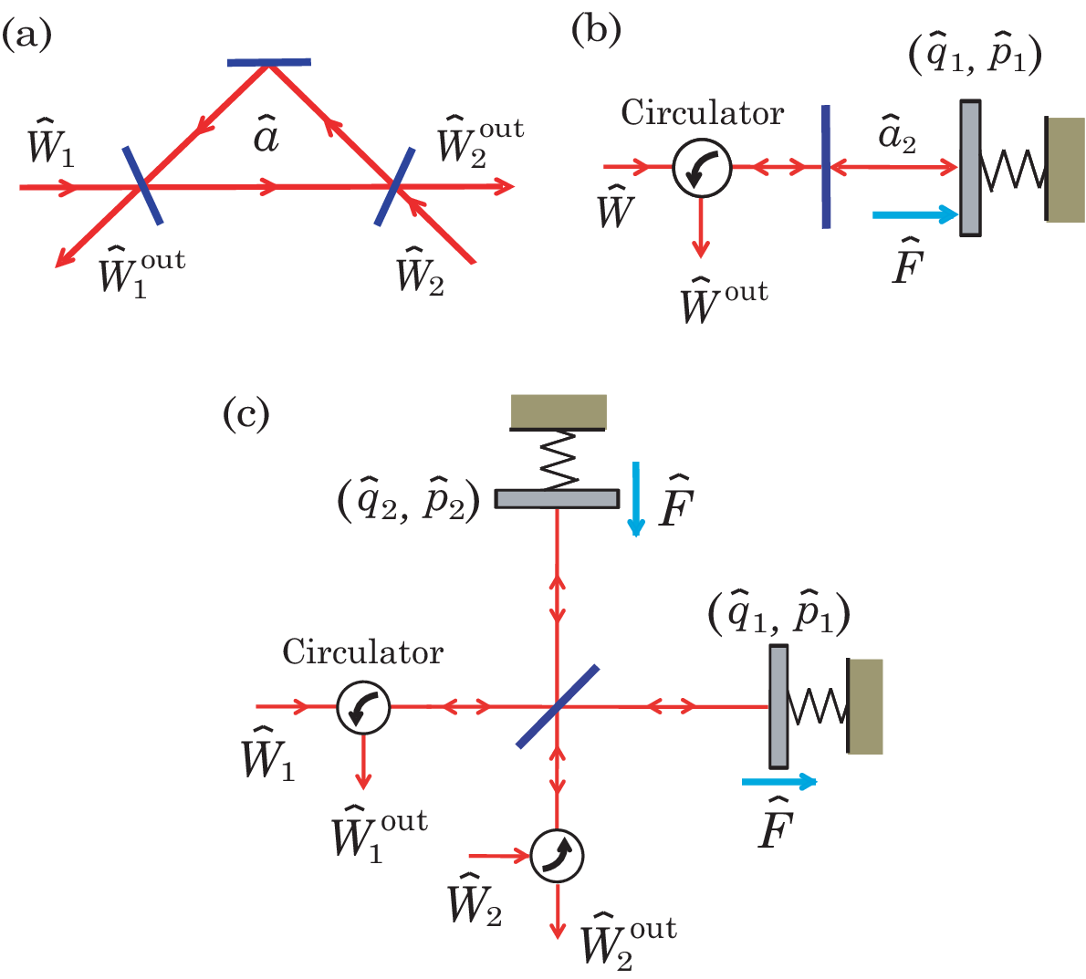
(i) A simple open linear system is an empty optical cavity with two input and output fields, depicted in Fig. 3 (a). The system equations are given by

$\hat{a}$ is the annihilation operator of the cavity mode. $\hat{A}_{j}$ and $\hat{A}_{j}^{\rm out}$ are the white noise operators of the $j$th incoming and the outgoing optical fields, respectively. $\kappa_{j}$ is the coupling strength between $\hat{a}$ and the $j$th field, which is proportional to the transmissivity of the coupling mirror. In this paper we express the variables in the quadrature form, which in this case are defined as $\hat{x}=[\hat{q},\hat{p}]^{\top}$ with $\hat{q}=(\hat{a}+\hat{a}^{*})/\sqrt{2}$ and $\hat{p}=(\hat{a}-\hat{a}^{*})/\sqrt{2}i$. Also $\hat{W}_{j}=[\hat{Q}_{j},\hat{P}_{j}]^{\top}$ with the field quadratures (15). Then, the above system equations are rewritten as

Typically this system works as a low-pass filter [50]; that is, for the noisy input field $\hat{W}_{1}$, the corresponding mode-cleaned output field $\hat{W}_{2}^{\rm out}$ is generated, which will be used later for e.g. some quantum information processing. To attain this goal, $\hat{W}_{1}^{\rm out}$ is measured to detect the error signal for locking the optical path length in the cavity. Note that $\hat{W}_{2}$ is a vacuum field. That is, in this case, the two input-output fields have different roles.

(ii) The mechanical oscillator shown in Fig. 3 (b) can also be modeled as a linear system. This system is composed of a mechanical oscillator with mode $(\hat{q}_{1},\hat{p}_{1})$ and a cavity with mode $\hat{a}_{2}=(\hat{q}_{2}+i\hat{p}_{2})/\sqrt{2}$. The cavity couples to a probe field $\hat{W}=[\hat{Q},\hat{P}]^{\top}$. After linearization, the system equation of $\hat{x}=[\hat{q}_{1},\hat{p}_{1},\hat{q}_{2},\hat{p}_{2}]^{\top}$ is obtained as

$m$ and $\omega$ are the mass and the resonant frequency of the oscillator. $\kappa$ is the coupling constant between the oscillator and the cavity field, which is proportional to the strength of radiation pressure force. $\gamma$ is the coupling constant between the cavity and the probe field. As indicated from the equations, it is possible to extract some information about the oscillator’s behavior by measuring the probe output field $\hat{W}^{\rm out}$. A typical situation is that the oscillator is pushed by an external force $\hat{F}$ with unknown strength; we attempt to estimate this value, by measuring $\hat{W}^{\rm out}$. The oscillator’s motion is usually much slower than that of the cavity field, thus we can adiabatically eliminate the cavity mode and have a reduced dynamical equation of only the oscillator:

where $\lambda=2\kappa^{2}/\gamma$ represents the strength of the direct coupling between the oscillator and the probe field. This equation clearly shows that only $\hat{P}^{\rm out}$ contains the information about the oscillator and accordingly $\hat{F}$; thus $\hat{P}^{\rm out}$ should be measured, implying $M_{1}=[0,1]$ in Eq. (17).

(iii) The last example is the Michelson’s interferometer composed of two identical mechanical oscillators with mass $m$ and resonant frequency $\omega$, depictd in Fig. 3 (c). This is a simplest configuration among various schemes that are expected to have capability of direct detection of a gravitational wave (GW) [38, 39, 56, 57]. A basic detection mechanism is as follows. A coherent light field $\hat{W}_{1}$ is injected into the left input port (bright port), while in the other port (dark port) the input $\hat{W}_{2}$ is set to be a vacuum. If a gravitational wave comes, one arm shrinks while the other one extends, thereby the oscillators experience tiny force along opposite directions, $\hat{F}$ and $-\hat{F}$. As a result the dynamics of the two oscillators can be modeled by the combination of Eq. (II.3):

Let us rewrite this equation in terms of the common modes $\hat{q}_{1}^{\prime}=(\hat{q}_{1}+\hat{q}_{2})/\sqrt{2},~\hat{p}_{1}^{\prime}=(\hat{p}_{1}+\hat{p}_{2})/\sqrt{2}$ and the differential modes $\hat{q}_{2}^{\prime}=(\hat{q}_{1}-\hat{q}_{2})/\sqrt{2},~\hat{p}_{2}^{\prime}=(\hat{p}_{1}-\hat{p}_{2})/\sqrt{2}$. Then these two modes are decoupled and the force $\hat{F}$ appears only in the dynamics of $\hat{x}_{2}^{\prime}=[\hat{q}_{2}^{\prime},\hat{p}_{2}^{\prime}]^{\top}$, which is exactly the same as Eq. (II.3):

Thus, ideally, by measuring $\hat{P}_{2}^{\rm out}$ we can detect $\hat{F}$.

The idea of BAE originally comes from the research for GW detection. The Michelson’s interferometer described in Sec. II-C is a simplest system for this purpose, and we now know from Eq. (II.3) that the measurement output $y=\hat{P}_{2}^{\rm out}=\sqrt{\lambda}\hat{q}_{2}^{\prime}+\hat{P}_{2}$ would offer some information about $\hat{F}$. The issue is that, in addition to the unavoidable noise $\hat{P}_{2}$ called the shot noise, the output $y$ contains the conjugate $\hat{Q}_{2}$, which is called the back-action (BA) noise, as seen explicitly in the Laplace domain:

The slight change of the oscillator’s position due to the GW effect, $\hat{g}$, is defined in the Fourier domain $s=i\Omega$ as $\hat{F}[i\Omega]=-mL\Omega^{2}\hat{g}[i\Omega]$, where $L$ is the optical path length in the interferometer. Hence under the assumption $\Omega\gg\omega$, the normalized signal containing $\hat{g}$ is given by

The noise power of $\tilde{y}$ is bounded from below by the following standard quantum limit (SQL):

The last inequality is due to the Heisenberg uncertainty relation $\langle{|\hat{Q}_{2}|^{2}}\rangle\langle{|\hat{P}_{2}|^{2}}\rangle\geq 1/4$. (For the simple notation, the power spectrum is defined without involving the delta function.) The SQL appears because the output $y$ contains the BA noise $\hat{Q}_{2}$ in addition to the shot noise $\hat{P}_{2}$. Thus, towards high-precision detection of $\hat{g}$, a special system configuration should be devised so that $y$ is free from $\hat{Q}_{2}$. That is, we need BAE. In fact, if BAE is realized, then by injecting a $\hat{P}_{2}$-squeezed light field into the dark port, we can possibly reduce the noise power below the SQL and may have chance to detect $\hat{g}$; for some specific configurations achieving BAE, see [38, 39, 52, 56, 57].

The above discussion can be generalized for the system (14) and (17). Let us assume that the signal to be detected is contained in the output (17):

Hence, $\hat{\cal Q}=M_{1}\hat{\cal W}$ is the shot noise, which must appear in $y$. The BA noise is then given by the conjugate $\hat{\cal P}=M_{2}\hat{\cal W}$. Note that these are vectors of operators: $\hat{\cal Q}=[\hat{Q}_{1},\ldots,\hat{Q}_{m}]^{\top}$ and $\hat{\cal P}=[\hat{P}_{1},\ldots,\hat{P}_{m}]^{\top}$. The matrices $M_{1}$ and $M_{2}$ satisfy several conditions (18); in particular $M_{1}^{\top}M_{1}+M_{2}^{\top}M_{2}=I$ holds and leads to $\hat{\cal W}=M_{1}^{\top}\hat{\cal Q}+M_{2}^{\top}\hat{\cal P}$. Hence Eq. (14) is rewritten as

BAE is realized, if the output (72) does not contain the BA noise $\hat{\cal P}$. (We will not consider the so-called variational measurement approach, in which case $M_{1}$ is frequency dependent.) In the language of linear systems theory, as stated in Eq. (8), this condition means that there is no subsystem that is controllable w.r.t. $\hat{\cal P}$ and observable w.r.t. $y$; i.e.

where ${\cal C}_{\hat{\cal P}}$ is the controllability matrix generated from $(A,\Sigma_{n}C^{\top}\Sigma_{m}M_{2}^{\top})$ and ${\cal O}_{y}$ is the observability matrix generated from $(A,M_{1}C)$. Further, again as described in Eq. (8), the condition (74) is equivalent to

Under this condition, the system equations (72) and (73) are represented in a transformed coordinate by

showing that actually there is no signal flow from $\hat{\cal P}$ to $y$. It is also obvious from this equation that, similar to the classical case (9), the equivalent characterization to Eq. (74) in terms of the transfer function is given by

Finally, note that achieving the above BAE condition (74) or (78) itself does not necessarily mean the improvement of signal sensitivity; actually in the case of GW force sensing discussed in Sec. VII-B, we need squeezing of the input field in addition to the BAE property for realizing such operational improvement.

Next to see the idea of QND variables, let us here study the atomic ensemble trapped in a cavity [1, 20, 70, 71] shown in Fig. 4. The atoms couple with a probe polarized light field, via the Faraday interaction. In terms of the total energy operator $\hat{J}_{z}$ and its conjugates $\hat{J}_{x}$ and $\hat{J}_{y}$, which satisfy the CCRs e.g. $\hat{J}_{y}\hat{J}_{z}-\hat{J}_{z}\hat{J}_{y}=i\hat{J}_{x}$, the ideal dynamics of atomic ensemble is described by

$\hat{P}$ is the phase quadrature of the input field’s noise operator corresponding to the polarization, and $M$ represents the coupling strength between the atoms and the field. In this setting, the amplitude quadrature of the output field should be measured, giving the following measurement output equation:

From these two equations, we find that, through the Faraday interaction, the polarization of the probe field rotates depending on the total energy $\hat{J}_{z}$, but $\hat{J}_{z}$ itself does not change; that is, $\hat{J}_{z}$ is a QND variable that can be measured without being disturbed. Typically $M$ is relatively small, and then the system variables obey a skew-Hermitian dynamics, implying that they preserve $\hat{J}_{x}^{2}+\hat{J}_{y}^{2}+\hat{J}_{z}^{2}$. Hence, in the large ensemble limit and in the short time period, the dynamics is constrained in the tangent space of this super-sphere with radius $J=N/2$ ($N$ is the number of atoms). In particular let us set $\hat{J}_{x}$ to be a constant $J$ rather than the operator-valued variable. Then the system variables are given by the usual CCR pairs $\hat{q}=\hat{J}_{y}/\sqrt{J}$ and $\hat{p}=\hat{J}_{z}/\sqrt{J}$ satisfying $\hat{q}\hat{p}-\hat{p}\hat{q}=i$, and the above system dynamics can be simplified to the following linear equation:

where $\mu=2MJ$. Clearly, $\hat{p}$ is not disturbed by the noise while it appears in the output signal, thus $\hat{p}$ is a QND variable. A merit of QND measurement is in the application to state preparation; if a QND variable exists, it is sometimes possible to deterministically stabilize its eigenstate by feedback [1], which can be highly non-classical such as a spin-squeezed state [20, 70].

As in the BAE case, we have a general characterization of the linear system (14) and (17) having a QND variable. Let $\hat{r}=v^{\top}\hat{x}$ be a QND variable with $v\in{\mathbb{R}}^{2n}$. Then, by definition, $\hat{r}$ must not be affected by the input field $\hat{\cal W}$, while it appears in the output signal (17), $y=MC\hat{x}+M\hat{\cal W}$. This means that, in the language of linear systems theory, $\hat{r}=v^{\top}\hat{x}$ is uncontrollable w.r.t. $\hat{\cal W}$ and observable w.r.t. $y$. Thus, the iff condition for a QND variable to exist is given by

and the vector $v$ lives in this intersection. Here, ${\cal C}_{\hat{\cal W}}$ and ${\cal O}_{y}$ are the controllability and observability matrices of the system (14) and (17). Note that the condition $v\in{\rm Ker}({\cal C}_{\hat{\cal W}}^{\top})$ can be explicitly represented by

Now let us collect QND variables into a single vector $\hat{x}_{2}^{\prime}$. Then, as described in Sec. II-A, $\hat{x}_{2}^{\prime}$ constitutes an uncontrollable subsystem w.r.t. $\hat{\cal W}$, which can be clearly seen in the transformed coordinate:

Note $C_{2}\neq 0$ due to the observability condition. Hence, $\hat{x}^{\prime}_{2}$ is free from $\hat{\cal W}$, while it appears in $y$. Remarkably, $\hat{x}^{\prime}_{2}$ obeys the closed dynamics $d\hat{x}_{2}^{\prime}/dt=A_{22}\hat{x}_{2}^{\prime}$; thus $\hat{x}^{\prime}_{2}$ is a generalization of a standard QND variable, which is usually considered to be static (i.e. $\hat{x}_{2}^{\prime}(t)=x_{2}^{\prime}(0)$, $\forall t$); see [72] for further detailed discussion. The above equation now enables us to obtain the equivalent condition to Eq. (80) in terms of the transfer functions:

The idea of the third control goal, generation of a DFS, can be clearly seen from the work [61], which studies a quantum memory served by an atomic ensemble in a cavity. Each atom has $\Lambda$-type energy levels, constituted by two metastable ground states $(|{s}\rangle,|{g}\rangle)$ and an excited state $|{e}\rangle$. The state transition between $|{e}\rangle$ and $|{g}\rangle$ is naturally coupled to the cavity mode $\hat{a}_{1}$ with strength $g\sqrt{N}$ ($N$ denotes the number of atoms), while the $|{s}\rangle\leftrightarrow|{e}\rangle$ transition is induced by a classical magnetic field with time-varying Rabi frequency $\omega(t)$. The system variables are the polarization operator $\hat{a}_{2}=\hat{\sigma}_{ge}/\sqrt{N}$ and the spin-wave operator $\hat{a}_{3}=\hat{\sigma}_{gs}/\sqrt{N}$, where $\hat{\sigma}_{\bullet}$ is the collective lowering operator; in a large ensemble limit, they can be well approximated by annihilation operators. Consequently the system dynamics is given by

References

- [1] H. M. Wiseman and G. J. Milburn, Quantum Measurement and Control (Cambridge University Press, 2010)
- [2] A. Barchielli and M. Gregoratti, Quantum Trajectories and Measurements in Continuous Time: The Diffusive Case, Lect. Notes Phys. 782 (Springer, Berlin, 2009)
- [3] L. Bouten, R. van Handel, and M. R. James, A discrete invitation to quantum filtering and feedback control, SIAM Review 51, 239/316 (2009)
- [4] V. P. Belavkin, Quantum stochastic calculus and quantum nonlinear filtering, J. Multivariate Anal. 42, 171 (1992)
- [5] V. P. Belavkin, Quantum diffusion, measurement and filtering I, Theor. Probab. Appl. 38, 573 (1993)
- [6] L. Bouten, R. van Handel, and M. R. James, An introduction to quantum filtering, SIAM J. Contr. Optim. 46-6, 2199/2241 (2007)
- [7] T. Kailath, Linear Systems (Englewood Cliffs, NJ: Prentice-Hall, 1980)
- [8] W. M. Wonham, Linear Multivariable Control: A Geometric Approach, 3rd ed. (Springer-Verlag, 1985)
- [9] K. Zhou and J. C. Doyle, Essentials of Robust Control (Prentice Hall, 1997)
- [10] A. C. Doherty and K. Jacobs, Feedback control of quantum systems using continuous state estimation, Phys. Rev. A 60, 2700 (1999)
- [11] A. Hopkins, K. Jacobs, S. Habib, and K. Schwab, Feedback cooling of a nanomechanical resonator, Phys. Rev. B 68, 235328 (2003)
- [12] R. Hamerly and H. Mabuchi, Advantages of coherent feedback for cooling quantum oscillators, Phys. Rev. Lett. 105, 123601 (2013)
- [13] R. Hamerly and H. Mabuchi, Coherent controllers for optical-feedback cooling of quantum oscillators, Phys. Rev. A 87, 013815 (2013)
- [14] C. Ahn, A. C. Doherty, and A. J. Landahl, Continuous quantum error correction via quantum feedback control, Phys. Rev. A 65, 042301 (2002)
- [15] H. Mabuchi, Continuous quantum error correction as classical hybrid control, New J. Phys. 11, 105044 (2009)
- [16] G. Tajimi and N. Yamamoto, Dynamical Gaussian state transfer with quantum error correction architecture, Phys. Rev. A 11, 022303 (2012)
- [17] C. Sayrin, et. al., Real-time quantum feedback prepares and stabilizes photon number states, Nature 477, 73 (2011)
- [18] R. Vijay, C. Macklin, D. H. Slichter, S. J. Weber, K. W. Murch, R. Naik, A. N. Korotkov, and I. Siddiqi, Stabilizing Rabi oscillations in a superconducting qubit using quantum feedback, Nature 490, 77 (2012)
- [19] S. Shankar et. al., Autonomously stabilized entanglement between two superconducting quantum bits, Nature 504, 419 (2013)
- [20] R. Inoue, S. Tanaka, R. Namiki, T. Sagawa, and Y. Takahashi, Unconditional quantum-noise suppression via measurement-based quantum feedback, Phys. Rev. Lett. 110, 163602 (2013)
- [21] H. M. Wiseman and G. J. Milburn, All-optical versus electro-optical quantum-limited feedback, Phys. Rev. A 49, 4110 (1994)
- [22] M. R. James, H. I. Nurdin, and I. R. Petersen, control of linear quantum stochastic systems, IEEE Trans. Automat. Contr. 53-8, 1787/1803 (2008)
- [23] J. E. Gough and M. R. James, The series product and its application to quantum feedforward and feedback networks, IEEE Trans. Automat. Contr. 54-11, 2530/2544 (2009)
- [24] H. I. Nurdin, M. R. James, and A. C. Doherty, Network synthesis of linear dynamical quantum stochastic systems, SIAM J. Control Optim. 48-4, 2686/2718 (2009)
- [25] J. E. Gough, M. R. James, and H. I. Nurdin, Squeezing components in linear quantum feedback networks, Phys. Rev. A 81, 023804 (2010)
- [26] M. Yanagisawa and H. Kimura, Transfer function approach to quantum control– Part I: Dynamics of quantum feedback systems, IEEE Trans. Automat. Contr. 48-12, 2107/2120 (2003)
- [27] J. E. Gough and S. Wildfeuer, Enhancement of field squeezing using coherent feedback, Phys. Rev. A 80, 42107 (2009)
- [28] J. Kerckhoff, H. I. Nurdin, D. Pavlichin, and H. Mabuchi, Designing quantum memories with embedded control: Photonic circuits for autonomous quantum error correction, Phys. Rev. Lett. 105, 040502 (2010)
- [29] H. Mabuchi, Coherent-feedback control strategy to suppress spontaneous switching in ultra-low power optical bistability, Appl. Phys. Lett. 98, 193109 (2011)
- [30] H. Mabuchi, Coherent-feedback quantum control with a dynamic compensator, Phys. Rev. A 78, 32323 (2008)
- [31] S. Iida, M. Yukawa, H. Yonezawa, N. Yamamoto, and A. Furusawa, Experimental demonstration of coherent feedback control on optical field squeezing, IEEE Trans. Automat. Contr. 57-8, 2045/2050 (2012)
- [32] O. Crisafulli, N. Tezak, D. B. S. Soh, M. A. Armen, and H. Mabuchi, Squeezed light in an optical parametric oscillator network with coherent feedback quantum control, Optics Express 21-15, 18372 (2013)
- [33] J. Kerckhoff et. al., Tunable coupling to a mechanical oscillator circuit using a coherent feedback network, Phys. Rev. X 3, 021013 (2013)
- [34] H. I. Nurdin, M. R. James, and I. R. Petersen, Coherent quantum LQG control, Automatica 45, 1837/1846 (2009)
- [35] K. Jacobs, X. Wang, and H. M. Wiseman, Coherent feedback that beats all measurement-based feedback protocols, New J. Phys. 16, 073036 (2014)
- [36] C. W. Gardiner and P. Zoller, Quantum Noise (Berlin: Springer, 2000)
- [37] D. F. Walls and G. J. Milburn, Quantum Optics, 2nd ed. (Springer, 2008)
- [38] V. B. Braginsky and F. Y. Khalili, Quantum Measurement (Cambridge University Press, Cambridge; New York, 1992)
- [39] C. M. Caves, K. S. Thorne, R. W. P. Drever, V. D. Sandberg, and M. Zimmermann, On the measurement of a weak classical force coupled to a quantum-mechanical oscillator, I, Issues of principle, Rev. Mod. Phys. 52, 341 (1980)
- [40] V. B. Braginsky, Y. I. Vorontsov, and K. S. Thorne, Quantum nondemolition measurements, Science 209, 547 (1980).
- [41] P. Zanardi and M. Rasetti, Noiseless quantum codes, Phys. Rev. Lett. 79, 3306 (1997)
- [42] D. A. Lidar and K. B. Whaley, Decoherence-free subspaces and subsystems, Irreversible Quantum Dynamics, ed. F. Benatti and R. Floreanini (Berlin: Springer) Lect. Notes Phys. 622, 83 (2003)
- [43] J. M. Courty, A. Heidmann, and M. Pinard, Back-action cancellation in interferometers by quantum locking, Europhys. Lett. 63-2, 226/232 (2003)
- [44] J. M. Courty, A. Heidmann, and M. Pinard, Quantum locking of mirrors in interferometers, Phys. Rev. Lett. 90, 083601 (2003)
- [45] D. Vitali, M. Punturo, S. Mancini, P. Amico, and P. Tombesi, Noise reduction in gravitational wave interferometers using feedback, J. Opt. B: Quantum Semiclass. Opt. 6, 691 (2004)
- [46] H. M. Wiseman, Using feedback to eliminate back-action in quantum measurements, Phys. Rev. A 51, 2459 (1995)
- [47] F. Ticozzi and L. Viola, Quantum Markovian subsystems: Invariance, attractivity and control, IEEE Trans. Automat. Contr. 53-9, 2048/2063 (2008)
- [48] F. Ticozzi and L. Viola, Analysis and synthesis of attractive quantum Markovian dynamics, Automatica 45-9, 2002/2009 (2009)
- [49] S. G. Schirmer and X. Wang, Stabilizing open quantum systems by Markovian reservoir engineering, Phys. Rev. A 81, 062306 (2010)
- [50] H. A. Bachor and T. C. Ralph, A Guide to Experiments in Quantum Optics (Weinheim, Wiley-VCH, 2004)
- [51] C. K. Law, Interaction between a moving mirror and radiation pressure: A Hamiltonian formulation, Phys. Rev. A 51, 2537 (1995)
- [52] M. Tsang and C. M. Caves, Coherent quantum-noise cancellation for optomechanical sensors, Phys. Rev. Lett. 105, 123601 (2010)
- [53] Y. D. Wang and A. A. Clerk, Using dark modes for high-fidelity optomechanical quantum state transfer, New J. Phys. 14, 105010 (2012)
- [54] Y. D. Wang and A. A. Clerk, Using interference for high fidelity quantum state transfer in optomechanics, Phys. Rev. Lett. 108, 153603 (2012)
- [55] C. Dong, V. Fiore, M. C. Kuzyk, and H. Wang, Optomechanical dark mode, Science 338, 1609 (2012)
- [56] Y. Chen, Macroscopic quantum mechanics: Theory and experimental concepts of optomechanics, J. Phys. B: At. Mol. Opt. Phys. 46, 104001 (2013)
- [57] H. Miao, Exploring Macroscopic Quantum Mechanics in Optomechanical Devices (Springer, Berlin, 2012)
- [58] L. M. Duan, J. I. Cirac, and P. Zoller, Three-dimensional theory for interaction between atomic ensembles and free-space light, Phys. Rev. A 66, 023818 (2002)
- [59] D. N. Matsukevich, T. Chaneliere, S. D. Jenkins, S. Y. Lan, T. A. B. Kennedy, and A. Kuzmich, Deterministic single photons via conditional quantum evolution, Phys. Rev. Lett. 97, 013601 (2006)
- [60] A. S. Parkins, E. Solano, and J. I. Cirac, Unconditional two-mode squeezing of separated atomic ensembles, Phys. Rev. Lett. 96, 053602 (2006)
- [61] A. V. Gorshkov, A. Andre, M. D. Lukin, and A. S. Sorensen, Photon storage in Lambda-type optically dense atomic media, I. Cavity model, Phys. Rev. A 76, 033804 (2007)
- [62] K. Hammerer, A. S. Sorensen, and E. S. Polzik, Quantum interface between light and atomic ensembles, Rev. Mod. Phys. 82, 1041 (2010)
- [63] S. L. Braunstein and P. van Loock, Quantum information with continuous variables, Rev. Mod. Phys. 77, 513 (2005)
- [64] A. Furusawa and P. van Loock, Quantum Teleportation and Entanglement: A Hybrid Approach to Optical Quantum Information Processing (Berlin: Wiley-VCH, 2011)
- [65] A. Ferraro, S. Olivares, and M. G. A. Paris, Gaussian states in continuous variable quantum information, arXiv:quant-ph/0503237 (2005)
- [66] C. Weedbrook, S. Pirandola, R. Garcia-Patron, N. J. Cerf, T. C. Ralph, J. H. Shapiro, and S. Lloyd, Gaussian quantum information, Rev. Mod. Phys. 84, 621 (2012)
- [67] G. J. Milburn, Coherent control of single photon states, Eur. Phys. J. 159, 113/117 (2008)
- [68] F. Khalili, S. Danilishin, H. Miao, H. Muller-Ebhardt, H. Yang, and Y. Chen, Preparing a mechanical oscillator in non-Gaussian quantum states, Phys. Rev. Lett. 105, 070403 (2010)
- [69] N. Yamamoto and M. R. James, Zero-dynamics principle for perfect quantum memory in linear networks, New J. Phys. 16, 073032 (2014)
- [70] J. K. Stockton, JM Geremia, A. C. Doherty, and H. Mabuchi, Robust quantum parameter estimation: Coherent magnetometry with feedback, Phys. Rev. A 69, 032109 (2004)
- [71] L. Bouten, J. K. Stockton, G. Sarma, and H. Mabuchi, Scattering of polarized laser light by an atomic gas in free space: A quantum stochastic differential equation approach Phys. Rev. A 75, 052111 (2007)
- [72] M. Tsang and C. M. Caves, Evading quantum mechanics: Engineering a classical subsystem within a quantum environment, Phys. Rev. X 2, 031016 (2012)
- [73] J. S. Prauzner-Bechcicki, Two-mode squeezed vacuum state coupled to the common thermal reservoir, J. Phys. A: Math. Gen. 37, 173 (2004)
- [74] G. Manzano, F. Galve, and R. Zambrini, Avoiding dissipation in a system of three quantum harmonic oscillators, Phys. Rev. A 87, 032114 (2013)
- [75] N. Yamamoto, Decoherence-free linear quantum subsystems, IEEE Trans. Automat. Contr. 59-7, 1845/1857 (2014)
- [76] M. H. Wimmer, D. Steinmeyer, K. Hammerer, and M. Heurs, Coherent cancellation of backaction noise in optomechanical force measurements, Phys. Rev. A 89, 053836 (2014)
- [77] H. M. Wiseman and G. J. Milburn, Quantum theory of field-quadrature measurements, Phys. Rev. A 47, 642 (1993)
- [78] A. Isidori, Nonlinear Control Systems, 3rd ed. (Springer, 1995)
- [79] H. Nijmeijer and A. van der Schaft, Nonlinear Dynamical Control Systems, 3rd ed. (Springer, 1996)
- [80] G. I. Harris, D. L. McAuslan, T. M. Stace, A. C. Doherty, and W. P. Bowen, Minimum requirements for feedback enhanced force sensing, Phys. Rev. Lett. 111, 103603 (2013)
- [81] H. M. Wiseman, Quantum theory of continuous feedback, Phys. Rev. A 49, 2133 (1994)