eurm10 \checkfontmsam10 \pagerange119–126
Ion and electron heating during magnetic reconnection in weakly collisional plasmas
Abstract
Magnetic reconnection and associated heating of ions and electrons in strongly magnetized, weakly collisional plasmas are studied by means of gyrokinetic simulations. It is shown that an appreciable amount of the released magnetic energy is dissipated to yield (irreversible) electron and ion heating via phase mixing. Electron heating is mostly localized to the magnetic island, not the current sheet, and occurs after the dynamical reconnection stage. Ion heating is comparable to electron heating only in high- plasmas, and results from both parallel and perpendicular phase mixing due to finite Larmor radius (FLR) effects; in space, ion heating is mostly localized to the interior of a secondary island (plasmoid) that arises from the instability of the current sheet.
52.35.Vd, 52.35.Py, 52.30.Gz, 52.65.Tt
1 Introduction
Magnetic reconnection is a commonly observed fundamental process in plasmas. It allows topological change of magnetic field lines, and rapidly converts the free energy stored in the magnetic field into various forms of energy. Amongst other poorly understood aspects of magnetic reconnection, such as explaining the explosive time scale that is often observed, or the onset mechanism, one key issue is the question of energy partition, i.e. understanding how, and how much of, the released energy is distributed into the different available channels: bulk heating of each of the plasma species and non-thermal particle acceleration.
Plasma heating is often observed to accompany magnetic reconnection in both astrophysical and laboratory plasmas (see, e.g. a recent review by Yamada et al. (2010)). Specifically, the measured ion temperature in reversed-field pinches (RFP), spheromaks, and merging plasma experiments where reconnection events are thought to be occurring (Ono et al., 1996; Hsu et al., 2001; Fiksel et al., 2009) often well exceeds the electron temperature. The fact that ions are selectively heated invalidates Ohmic dissipation of the current sheet as the dominant heating source since it primarily deposits the energy into current carrying electrons. Furthermore, heating associated with reconnection events generally occurs much faster than the expected time scale estimated from the Ohmic heating, as expected in weakly collisional environments. Various mechanisms causing such ‘anomalous’ ion heating have been suggested: Stochastic ion heating has been studied (Fiksel et al., 2009) for explaining ion heating in a RFP device where multiple reconnections in turbulent environments are occurring rather than a single reconnection event, while anomalous resistivity has been invoked in MRX (Hsu et al., 2001).
In the weakly collisional plasmas often found in reconnection environments, Ohmic and viscous heating cannot, by definition, be important. This leaves phase mixing as the only possible mechanism of converting energy from the fields to the particles in an irreversible way. Indeed, kinetic effects generally lead to non-Maxwellian distribution functions; once highly oscillatory structures are created in velocity space, they suffer strong collisional dissipation as the collision operator provides diffusion in velocity space. The thermalization time scale may be comparable to the time scale of magnetic reconnection; therefore, to address thermodynamic properties of such plasmas, collisional effects are essential, even though collisions are rare and not responsible for reconnection itself (i.e. the frozen flux condition is broken by electron kinetic effects, not collisions) 11 1 In the interest of clarity, notice that by ‘heating’ we mean the increase in the entropy of the system due to reconnection. Note that this definition excludes the energization of supra-thermal particles, a process that is sometimes also referred to as heating but which is formally reversible and does not, therefore, change the entropy of the system by itself. .
Landau damping (Landau, 1946) is one of the well-known examples of phase mixing, in which nearly synchronous particles with the electrostatic potential variations absorb energy from the field. Phase mixing occurs along the direction of electron free stream, i.e. along the magnetic field lines. The parallel phase mixing and resultant heating of electrons during magnetic reconnection in low- plasmas ( is the ratio of the plasma to the magnetic pressure) have been studied using a reduced kinetic model (Zocco & Schekochihin, 2011; Loureiro et al., 2013b) and the full gyrokinetic model (Numata & Loureiro, 2014), and the significance of such an effect has been proved.
Phase mixing can also be induced by a FLR effect (Dorland & Hammett, 1993). In strongly magnetized plasmas, particles undergo drifts (dominantly the drift) in the perpendicular direction to the mean magnetic field. Gyro-averaging of the fields will give rise to spread of the drift velocity of different particles, hence will lead to phase mixing in the perpendicular direction. Unlike linear parallel phase mixing of Landau damping, the FLR-phase-mixing process causes damping proportional to the field strength, and only appears nonlinearly (nonlinear phase mixing). Energy dissipation due to FLR phase mixing has been investigated in electrostatic turbulence (Tatsuno et al., 2009); its role in magnetic reconnection has never been studied.
In this paper, we present gyrokinetic simulations of magnetic reconnection using the numerical code AstroGK (Numata et al., 2010). Our main aim is to perform a detailed analysis of ion and electron (irreversible) heating in weakly collisional, strongly magnetized plasmas. We follow Numata et al. (2011) and Numata & Loureiro (2014) to setup a tearing-mode unstable configuration. In addition to the electron heating due to parallel phase mixing in low- plasmas as has already been shown in Loureiro et al. (2013b) and Numata & Loureiro (2014), ion heating is also expected to be significant in high- plasmas since compressible fluctuations will be excited which are strongly damped collisionlessly (Schekochihin et al., 2009). The main questions we are going to address will be (i) fraction of ion and electron heating, (ii) dissipation channel, i.e. how much energy is converted via phase mixing, resistivity and viscosity, and (iii) how the answer to the above questions scales with plasma beta. We also study in detail how and where plasma heating occurs via phase mixing, which may be important to the interpretation of plasma heating as measured in laboratory experiments or space and astrophysical plasmas.
This paper is organized as follows: We start with defining plasma heating and energy dissipation within the framework of the gyrokinetic model in Sec. 2. The details of the simulation setup and choices of parameters are described in Sec. 3. In the same section, simulations of the linear regime are presented to identify the region of parameter space where the tearing instability growth rate is independent of the plasma collisionality (the so-called collisionless regime of reconnection). In Sec. 4, we report the results of nonlinear simulations, focusing on the dependence on plasma beta of the reconnection dynamics, as well as on the detailed analysis of ion and electron heating caused by magnetic reconnection. We summarize the main results of this paper in Sec. 5.
2 Plasma heating and energy dissipation
We consider magnetic reconnection in the framework of gyrokinetics. Plasma heating is measured by the entropy production (irreversible), rather than increase of temperature (reversible) in this work. In the absence of collisions, the gyrokinetic equation conserves the generalized energy consisting of the particle part and the magnetic field part
| (1) |
The subscript (for ions) or (for electrons) denotes the species label. is the Maxwellian distribution function of background plasmas, , are the density and temperature, is the thermal velocity, , are the mass and electric charge. The perturbed distribution function is , where is the non-Boltzmann part obeying the gyrokinetic equation. , , are, respectively, the electrostatic potential, vector potential and perturbed magnetic field along the background magnetic field , and is the vacuum permeability. Note that the perturbed particle energy is , where is the perturbed entropy.
If we extract explicitly the first two velocity moments from as in Zocco & Schekochihin (2011),
| (2) |
where
| (3) |
the particle’s energy is decomposed into the density variance, the parallel kinetic energy, and the rest as follows:
| (4) |
The generalized energy is dissipated by collisions as , where the dissipation rate of each species is given by
| (5) |
The angle bracket denotes the gyro-averaging operation. The collision term is modeled by the linearized, and gyro-averaged, Landau collision operator (Abel et al., 2008; Barnes et al., 2009). It consists of like-particle collisions of electrons and ions whose frequencies are given by and , and inter-species collisions of electrons with ions given by ( is the effective ion charge, and is set to unity in this paper). The ion-electron collisions are subdominant compared with the ion-ion collisions. The electron-ion collisions reproduce Spitzer resistivity (Spitzer & Härm, 1953) for which the electron-ion collision frequency and the resistivity () are related by where is the electron skin depth.
The dissipation rate contains all possible dissipation channels. Besides the dissipation that can be modeled in fluid models, e.g. the resistivity, also contains dissipation of higher order velocity moments due to phase mixing depending on the form of .
In our problem setup explained in Sec. 3, the initial energy is contained in the perpendicular magnetic field energy and the electron parallel kinetic energy (i.e. the reconnecting magnetic field and the current associated with it). During the magnetic reconnection process, the initial energy is distributed into other forms of energy in a reversible way, and is only irreversibly dissipated from the system through collisions. There is no direct dissipation channel of the magnetic field energy. The resistive dissipation is the collisional decay of particle’s kinetic energy (current) supporting the magnetic field.
The increased entropy is turned into heat, and the background temperature increases on a time scale much longer than the time scale considered in the simulation (Howes et al., 2006). In this sense, we identify the energy dissipation (5) and plasma heating. The background temperature does not change during simulations.
3 Simulation setup
We consider magnetic reconnection of strongly magnetized plasmas in a two-dimensional doubly periodic slab domain. Simulations are carried out using the gyrokinetic code AstroGK (Numata et al., 2010). We initialize the system by a tearing unstable magnetic field configuration (see Numata et al. (2010); Numata et al. (2011) for details). The equilibrium magnetic field profile is
| (6) |
where is the background guide magnetic field and is the in-plane, reconnecting component, related to the parallel vector potential by , is the gyrokinetic epsilon – a small expansion parameter enabling scale separation in gyrokinetics (see, e.g. Howes et al. (2006)), and
| (7) |
( is a shape function to enforce periodicity (Numata et al., 2010).) is generated by the electron parallel current to satisfy the parallel Ampère’s law. The equilibrium scale length is denoted by and is the length of the simulation box in the direction, set to . In the direction, the box size is . We impose a small sinusoidal perturbation to the equilibrium magnetic field, with wave number , yielding a value of the tearing instability parameter . The background temperatures () and densities () are spatially uniform and held constant throughout the simulations. We consider a quasi-neutral plasma, so , and singly charged ions .
The equilibrium magnetic field defines the time scale of the system. We normalize time by the Alfvén time , where is the (perpendicular) Alfvén velocity corresponding to the peak value of .
We solve the fully electromagnetic gyrokinetic equations for electrons and ions. AstroGK employs a pseudo-spectral algorithm for the spatial coordinates (), and Gaussian quadrature for velocity space integrals. The velocity space is discretized in the energy and . The velocity space derivatives in the collision operator are estimated using a first order finite difference scheme on an unequally spaced grid according to the quadrature rules (Barnes et al., 2009).
3.1 Parameters
There are four basic parameters in the system: The mass ratio, , the temperature ratio of the background plasma, , the electron plasma beta, , and the ratio of the ion sound Larmor radius to the equilibrium scale length , . The ion sound speed for cold ions is , and the ion cyclotron frequency is . Those parameters define the physical scales associated with the non-magnetohydrodynamic effects:
| (8) | ||||||
| (9) |
where and are the ion and electron Larmor radii and skin depths, respectively.
We fix the following parameters throughout this paper:
| (10) |
Therefore, , , and . We scan in from 0.01 to 1; the electron inertial length also changes accordingly as shown in Table 1. The ion inertial length is always .
| Case | |||
| 1 | 0.01 | 0.25 | |
| 2 | 0.03 | 0.14 | |
| 3 | 0.1 | 0.079 | |
| 4 | 0.3 | 0.046 | |
| 5 | 1 | 0.025 |
To identify the collisionless tearing-mode regime (i.e. such that the frozen-flux condition is not broken by collisions but instead by the electron inertia or electron FLR effects), we perform linear simulations. For the linear runs, we take the number of collocation points in the pitch angle direction () and the energy direction () as ; the number of grid points in the direction ranges from 256 to 1024, and we consider a single mode in the direction (the fastest growing mode for this configuration). We have verified that these numbers provide adequate resolution.
Shown in Fig. 1 are the growth rates () and current layer widths () as functions of collisionality. For comparison, we also show the growth rate and current layer width for obtained from the reduced kinetic model valid for using the Viriato code (Loureiro et al., 2013b); the agreement with the fully-gyrokinetic results at is very good.
As collisionality decreases, the growth rate also decreases, and the current layer becomes narrower. However, when collisionality becomes sufficiently small, the growth rate and the current layer width asymptote to constant values. This is the so-called collisionless regime, even though the collision frequency is finite. Note that, in the linear regime, small but finite collisionality gives the same results as the exactly collisionless case .


Figure 2 shows the growth rate and current layer width for the collisionless cases against . The growth rate decreases with increasing , scaling roughly as (), as predicted by Fitzpatrick (2010) based on Braginskii’s two-fluid model 22 2 If is much smaller, or is much larger, the other collisionless regime originally derived by Porcelli (1991), (), appears – see Numata et al. (2011).. The dependence of the current layer width indicates the physical mechanism responsible for breaking the frozen-flux constraint. For , the electron Larmor radius is negligibly small compared with , and reconnection is mediated by electron inertia. As increases, the current layer width decreases, and becomes comparable to and . For , becomes larger than , and, thus, electron FLR effects overtake electron inertia as the mechanism for breaking the flux-freezing condition.

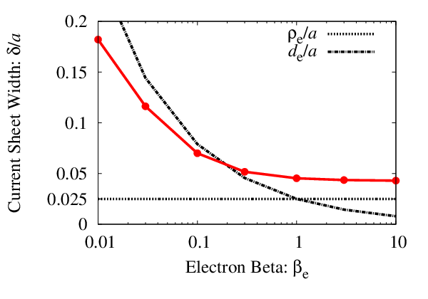
4 Nonlinear simulation results
We now report the results of nonlinear simulations in the collisionless regime at different values of . We set (see Table 1) 11 1 The ion-ion collisions do not significantly affect the reconnection dynamics, and are just included to regularize velocity space structures of the ion distribution function. An ion collision frequency equal to the electron one is assumed to be sufficient since the ion phase mixing is at most as strong as that of electrons. Ideally, a similar convergence test for ions as electrons shown in Appendix A should be performed. .
In all simulations reported here, the number of grid points in the , directions are , (subject to the 2/3’s rule for de-aliasing), except for , where such that the linear stage can be adequately resolved. In velocity space, we use for all cases, as required by the convergence test described in Appendix A.
4.1 Temporal evolution of magnetic reconnection
Figure 3 shows the time evolution of the electric field at the point () as a measure of the reconnection rate for different values of . The peak reconnection rate values that we find () are comparable with the standard value usually reported in the literature in the no-guide-field case; in addition, we find that the peak reconnection rate is a weakly decreasing function of . The reconnection rate from Viriato is again showing very good agreement with the case. For higher cases, the electric field drops sharply shortly after the peak reconnection rate is achieved, eventually reversing sign; this occurs because the current sheet becomes unstable to the secondary plasmoid instability (Loureiro et al., 2007; Loureiro et al., 2013a), with the point becoming an point instead – see Fig. 9 for the case. In the simulations shown in this work, the secondary island stays at the center of the domain because there is no asymmetry in the direction of the reconnecting field lines (i.e. the outflow direction). For the case, however, it eventually moves toward the primary island due to the numerical noise as indicated by the sharp spike of around .


To detail the energy conversion processes taking place in our simulations we plot in Fig. 4 the time evolution of each component of the generalized energy (1) normalized by the initial magnetic energy (), except the parallel magnetic energy () as it is almost zero for all cases.


During magnetic reconnection, the magnetic energy is converted to the particle’s energy reversibly. Looking at the case we see that, first, the ion drift flow is excited, thereby increasing the ion energy. Then, electrons exchange energies with the excited fields. The parallel electric field accelerates or decelerates electrons depending on their orbit and energy, but the net work done on electrons for this case is positive. Even though electrons lose parallel kinetic energy by resistive dissipation, they gain energy via the phase-mixing process as will be explained in detail shortly, and store the increased energy in the form of temperature fluctuations and higher order moments. Collisionally dissipated energy (decrease of the total energy) is about 1% of the initial magnetic energy after dynamical process has almost ended ().
Also shown in Fig. 4, right panel, are the dissipation rates of electrons and ions as determined from (5). The dissipation rate is normalized by the initial magnetic energy divided by the Alfvén time, . For , the electron energy dissipation starts to grow rapidly when the maximum reconnection rate is achieved. It stays large long after the dynamical stage, and an appreciable amount of the energy is lost at late times. The ion dissipation is negligibly small compared with the electron’s for this case.
With regards to energy partition, the most important effect to notice as increases is the decrease in the electron energy gain. For the case, the released magnetic energy is contained mostly by ions as shown in Fig. 4, bottom left.
The plasmoid formation and ejection complicate the evolution of energies and dissipations for the case. From the bottom-left panel of Fig. 4, we notice that there is a slight increase of the magnetic energy during the plasmoid growth phase (). The electron dissipation decreases in this phase, and is re-activated when the plasmoid is ejected (Fig. 4, bottom right). This secondary heating of electrons is associated with the newly formed point as will be shown in Fig. 13.
A significant fraction of the released magnetic energy is collisionally dissipated. The fraction of the dissipated energy [] to the released magnetic energy [] is shown in Fig. 5. The cross () and dot () symbols on each line indicate the times of the maximum reconnection rate and the maximum electron dissipation rate, respectively. We show only in the nonlinear regime since both and are almost zero in the linear regime (see Fig. 4).

The total energy dissipation is determined by the local strength of phase mixing (the magnitude of the integrand of (5) integrated over only the velocity coordinates at each position), the total area where phase mixing is active, and the duration of phase mixing. Therefore, the energy conversion from the magnetic to thermal energy (i.e. how much of the released magnetic energy is dissipated from the system ()) as a function of time has no clear dependence on . For the case, in particular, evolves in a complex manner because the evolution of energies and dissipations are significantly altered by the plasmoid as described above.
As is increased, the ion dissipation also becomes large. As shown in Fig. 6, the ratio of the energy dissipation of ions to electrons, , becomes approximately unity for the case implying that ion heating is as significant as electron heating when .

4.2 Phase mixing and energy dissipation
Figure 7 shows spatial distributions of the dissipation rate of electrons for . The top two panels show the dissipation rate of the electron energy at , i.e. when the reconnection rate is maximum. At this time, the electron dissipation is localized near the reconnection point. If we subtract the first two velocity moments from the distribution function, which correspond to perturbations of the density and bulk flow in the direction (i.e. the dissipation rate based on defined in (2)), we find that the dissipation occurs just downstream of the reconnection site. This indicates that the dissipation at the point is the resistivity component, corresponding to the decay of the initial electron current. The contribution of higher order moments to the dissipation spreads along the separatrix. The energy lost via Ohmic heating at this stage is much smaller than the dissipation due to phase mixing that occurs later, and is not seen in later times. (In all other plots of the spatial distribution of , the resistivity component is negligible.)
After the dynamical reconnection phase ended, most of the available flux has been reconnected and a large island is formed. Electron dissipation is large inside the island (bottom panel of Fig. 7), and continuously increases in time – see Fig. 4, top right.
In the regions where the dissipation rate is large, we expect the distribution function to show oscillatory structures due to phase mixing (the local strength of dissipation is roughly proportional to where denotes the scale length of the distribution function in velocity space). Figure 8 shows electron distribution functions, without the first two velocity moments, taken where the non-resistive part of dissipation rate is largest for . The distribution function is normalized by . The distribution function only has gradients in the direction, indicating that parallel phase mixing is occurring, and the scale length becomes smaller as time progresses. The phase-mixing structures develop slowly compared with the time scale of the dynamical reconnection process, therefore the energy dissipation peaks long after the peak reconnection rate (Loureiro et al., 2013b).
Phase mixing is significant when the Landau resonance condition is met: Electrons moving along the reconnected field lines feel variations of the electromagnetic fields evolving with the velocity in the perpendicular plane. Since the magnetic field lies dominantly in the direction, but has a small component in the plane, when electrons run along the field lines with , electrons also move in the plane with , thus the resonance condition is given by . For Fig. 8, phase mixing is most pronounced around , which agrees with the resonance condition for and the mass ratio . Therefore, electrons with can effectively exchange energies with the fields ( in this case because is small).
Parallel heating driven by the curvature drift through the Fermi acceleration mechanism suggested by Drake et al. (2006) and Dahlin et al. (2014) is negligible for the strong-guide-field case discussed here simply because the curvature drift is small compared with the thermal velocity.


For the case, we perform the same diagnostics for both electrons and ions in Figs. 9–12. For this case, the electron dissipation occurs, again, along the separatrix, but confined in narrow strips. At later times, the electron heating is restricted to the narrow edge region of the primary island. Looking at the structure of the electron distribution function at the point where the dissipation is largest, we see narrow parallel phase-mixing structures. The Landau resonance is pronounced for . Note that . More electrons are, thus, in resonance at higher-, thereby enhancing the local strength of phase mixing as an energy dissipation process.
At late times, the ion and electron dissipation rates become comparable. We show spatial distributions of the ion dissipation rate at the time of maximum reconnection rate, , and maximum of the ion dissipation rate, , in Fig. 11. It is clearly shown that the ion dissipation is localized to the center of the domain. While the reconnection process proceeds, ion flows in the direction develop as well as the drift in the plane. Collisional damping of those flows (ion viscosity) are the main contributions to the ion dissipation at , though this is only a small fraction of the dissipation that occurs later as a result of phase mixing. As shown in the distribution function plot in Fig. 12, the ion distribution function has a component proportional to driven by , and peaks at , corresponding to the drift velocity. No phase-mixing structures are visible at this time. At later times, the ion dissipation is large in the secondary island at the center of the domain. At this stage, the ion distribution function displays significant structure both in the parallel and perpendicular velocity directions, indicating that the overall dissipation is due to both parallel (linear) and perpendicular (nonlinear) phase mixing. Perpendicular phase mixing is indeed expected to be large for since . However, since it is a nonlinear dissipation mechanism, perpendicular phase mixing can only be significant when the amplitudes of the perturbed fields become sufficiently large.


Around , the secondary island moves due to the numerical noise, and the electron dissipation significantly increases. Spatial distributions of the dissipation rate of electrons and ions at this time are shown in Fig. 13. We see that the electron dissipation at this time occurs at the newly formed point, and is stronger compared with that at earlier times, indicating re-activation of the heating process. The ion dissipation does not significantly increase at the plasmoid ejection, but just spreads outside the secondary plasmoid.


5 Conclusion
We have reported gyrokinetic simulations of magnetic reconnection in weakly collisional, strongly magnetized plasmas at varying values of .
The peak reconnection rate we find is , as is often reported in the weak-guide-field case, and weakly decreases with increasing . We also observe that, as increases, the reconnection site becomes unstable to secondary island formation.
During reconnection, phase-mixing structures slowly develop. Electron heating occurs after the dynamical reconnection process has ceased, and continues long after. The ion heating is comparable to the electron heating for , and insignificant at lower values of . The fraction of energy dissipation to released magnetic energy is a complicated function of the local strength, area, and duration of the phase-mixing process.
The electron heating that we measure in our simulations is caused by parallel phase mixing. It initially occurs along the separatrix, and slowly spreads to the interior of the primary magnetic island. Phase mixing is most pronounced for electrons streaming along the magnetic field at velocities , where is the perpendicular Alfvén velocity. For our lowest case, this implies , whereas at larger the resonance condition is satisfied for . Consequently, electron dissipation is more efficient at higher values of . The ion heating, on the other hand, does not spread, as long as the plasmoid is stationary, occurring only at the reconnection site, and later inside the secondary island that is formed. For ions, both parallel and perpendicular phase-mixing processes are active. It is also found that, once the secondary island moves, the electron heating becomes active at the new point.
In summary, we have shown that electron and ion bulk heating via phase mixing is a significant energy dissipation channel in strong-guide-field reconnection, extending the results first reported in Loureiro et al. (2013b) to the regime of . These results, therefore, underscore the importance of retaining finite collisions in reconnection studies, even if the reconnection process itself is collisionless.
In addition, it is perhaps worth noting that the usual particle
energization mechanisms found in weak-guide-field reconnection (Fermi
acceleration (Drake et al., 2006)) cannot be efficient for
reconnection in strongly magnetized plasmas because the curvature drift
associated with the Fermi mechanism is small.
Our results may therefore point to an alternative heating mechanism valid
when the guide field is much larger than the reconnecting field. Scaling
studies such as those by TenBarge et al. (2014) may help
identify the regions of parameter space where each of these mechanisms
(Fermi or phase mixing) predominates.
Acknowledgements
This work was supported by JSPS KAKENHI Grant Number 24740373. This work was carried out using the HELIOS supercomputer system at Computational Simulation Centre of International Fusion Energy Research Centre (IFERC-CSC), Aomori, Japan, under the Broader Approach collaboration between Euratom and Japan, implemented by Fusion for Energy and JAEA. N. F. L. was supported by Fundação para a Ciência e a Tecnologia through grants Pest-OE/SADG/LA0010/2011, IF/00530/2013 and PTDC/FIS/118187/2010.
Appendix A Velocity space convergence
To determine the velocity-space resolution required to accurately capture electron and ion heating in our weakly collisional simulations, we perform a convergence test for the case. We run for . Plotted in Fig. A.1 are the dissipation rates of electrons with several velocity-space grid sizes. In the linear phase, , there is no phase mixing and, therefore, a relatively coarse velocity-space grid is sufficient. However, for the most collisionless case , we see that the velocity-space resolution greatly affects the dissipation rate in the nonlinear stage, as expected due to the development of fine velocity scales. For the most collisionless case, the number of velocity grid points must be greater than , while is sufficient for the more collisional cases.

References
- Abel et al. (2008) Abel, I. G., Barnes, M., Cowley, S. C., Dorland, W. & Schekochihin, A. A. 2008 Linearized model Fokker-Planck collision operators for gyrokinetic simulations I. Theory. Phys. Plasmas 15 (12), 122509.
- Barnes et al. (2009) Barnes, M., Abel, I. G., Dorland, W., Ernst, D. R., Hammett, G. W., Ricci, P., Rogers, B. N., Schekochihin, A. A. & Tatsuno, T. 2009 Linearized model Fokker-Planck collision operators for gyrokinetic simulations II. Numerical implementation and tests. Phys. Plasmas 16 (7), 072107.
- Dahlin et al. (2014) Dahlin, J. T., Drake, J. F. & Swisdak, M. 2014 The mechanisms of electron heating and acceleration during magnetic reconnection. Phys. Plasmas 21 (9), 092304.
- Dorland & Hammett (1993) Dorland, W. & Hammett, G. W. 1993 Gyrofluid turbulence models with kinetic effects. Phys. Fluids B 5 (3), 812–835.
- Drake et al. (2006) Drake, J. F., Swisdak, M., Che, H. & Shay, M. A. 2006 Electron acceleration from contracting magnetic islands during reconnection. Nature 443 (5), 553–556.
- Fiksel et al. (2009) Fiksel, G., Almagri, A. F., Chapman, B. E., Mirnov, V. V., Ren, Y., Sarff, J. S. & Terry, P. W. 2009 Mass-dependent ion heating during magnetic reconnection in a laboratory plasma. Phys. Rev. Lett. 103 (14), 145002.
- Fitzpatrick (2010) Fitzpatrick, R. 2010 Magnetic reconnection in weakly collisional highly magnetized electron-ion plasmas. Phys. Plasmas 17 (4), 042101.
- Howes et al. (2006) Howes, G. G., Cowley, S. C., Dorland, W., Hammett, G. W., Quataert, E. & Schekochihin, A. A. 2006 Astrophysical gyrokinetics: Basic equations and linear theory. Astrophys. J. 651 (1), 590–614.
- Hsu et al. (2001) Hsu, S. C., Carter, T. A., Fiksel, G., Ji, H., Kulsrud, R. M. & Yamada, M. 2001 Experimental study of ion heating and acceleration during magnetic reconnection. Phys. Plasmas 8 (5), 1916–1928.
- Landau (1946) Landau, L. D. 1946 On the vibrations of the electronic plasma. Zh. Eksp. Teor. Fiz. 16 (7), 574–586.
- Loureiro et al. (2007) Loureiro, N. F., Schekochihin, A. A. & Cowley, S. C. 2007 Instability of current sheets and formation of plasmoid chains. Phys. Plasmas 14 (10), 100703.
- Loureiro et al. (2013a) Loureiro, N. F., Schekochihin, A. A. & Uzdensky, D. A. 2013a Plasmoid and Kelvin-Helmholtz instabilities in Sweet-Parker current sheets. Phys. Rev. E 87, 013102.
- Loureiro et al. (2013b) Loureiro, N. F., Schekochihin, A. A. & Zocco, A. 2013b Fast collisionless reconnection and electron heating in strongly magnetised plasmas. Phys. Rev. Lett. 111 (2), 025002.
- Numata et al. (2011) Numata, R., Dorland, W., Howes, G. G., Loureiro, N. F., Rogers, B. N. & Tatsuno, T. 2011 Gyrokinetic simulations of the tearing instability. Phys. Plasmas 18 (11), 112106.
- Numata et al. (2010) Numata, R., Howes, G. G., Tatsuno, T., Barnes, M. & Dorland, W. 2010 AstroGK: Astrophysical gryokinetics code. J. Comput. Phys. 229 (24), 9347–9372.
- Numata & Loureiro (2014) Numata, R. & Loureiro, N. F. 2014 Electron and ion heating during magnetic reconnection in weakly collisional plasmas. JPS Conf. Proc. 1, 015044.
- Ono et al. (1996) Ono, Y., Yamada, M., Akao, T., Tajima, T. & Matsumoto, R. 1996 Ion acceleration and direct ion heating in three-component magnetic reconnection. Phys. Rev. Lett. 76 (18), 3328–3331.
- Porcelli (1991) Porcelli, F. 1991 Collisionless tearing mode. Phys. Rev. Lett. 66 (4), 425–428.
- Schekochihin et al. (2009) Schekochihin, A. A., Cowley, S. C., Dorland, W., Hammett, G. W., Howes, G. G., Quataert, E. & Tatsuno, T. 2009 Astrophysical gyrokinetics: Kinetic and fluid turbulent cascades in magnetized weakly collisional plasmas. Astrophys. J. Suppl. Ser. 182 (1), 310–377.
- Spitzer & Härm (1953) Spitzer, Jr., L. & Härm, R. 1953 Transport phenomena in a completely ionized gas. Phys. Rev. 89 (5), 977–981.
- Tatsuno et al. (2009) Tatsuno, T., Dorland, W., Schekochihin, A. A., Plunk, G. G., Barnes, M., Cowley, S. C. & Howes, G. G. 2009 Nonlinear phase mixing and phase-space cascade of entropy in gyrokinetic plasma turbulence. Phys. Rev. Lett. 103 (1), 015003.
- TenBarge et al. (2014) TenBarge, J. M., Daughton, W., Karimabadi, H., Howes, G. G. & Dorland, W. 2014 Collisionless reconnection in the large guide field regime: Gyrokinetic versus particle-in-cell simulations. Phys. Plasmas 21 (2), 020708.
- Yamada et al. (2010) Yamada, M., Kulsrud, R. & Ji, H. 2010 Magnetic reconnection. Rev. Mod. Phys. 82 (1), 603–664.
- Zocco & Schekochihin (2011) Zocco, A. & Schekochihin, A. A. 2011 Reduced fluid-kinetic equations for low-frequency dynamics, magnetic reconnection and electron heating in low-beta plasmas. Phys. Plasmas 18 (10), 102309.