Reachability Analysis of Quantum Markov Decision Processes

For convenience of the reader, we very briefly recall some basic notions in quantum theory with the main aim being fixing notations; see [25] for details. In this paper we always assume that the state Hilbert space is $d-$dimensional, i.e. $\mathcal{H}=\mathbb{C}^{d}$ where $\mathbb{C}$ is the field of complex numbers. We use the Dirac notation and assume that $\{|i\rangle\}_{i=1}^{d}$ is an orthonormal basis of $\mathcal{H}$. Then we have $\mathcal{H}={\rm span}\{|i\rangle\}$, a pure state in $\mathcal{H}$ can be written as $|\psi\rangle=\sum\alpha_{i}|i\rangle$ with $\sum|\alpha_{i}|^{2}=1$, and a mixed state is represented by a density matrix in $\mathcal{H}$, i.e. a semi-definite positive $d\times d$ matrix with trace $1$. Write $\mathcal{D}(\mathcal{H})$ for the set of all density matrices in $\mathcal{H}$. The identity matrix is denoted $I$. If a density matrix can be written as $\rho=\sum p_{i}|\psi_{i}\rangle\langle\psi_{i}|$, where $\langle\psi_{i}|$ stands for the transpose conjugate of $|\psi_{i}\rangle$, then its support is ${\rm supp}(\rho)={\rm span}\{|\psi_{i}\rangle:p_{i}>0\}$.

The evolution of a closed quantum system is described by a $d\times d$ unitary matrix: $|\phi\rangle\mapsto U|\phi\rangle$. A super-operator ${\mathcal{E}}:\mathcal{D}(\mathcal{H})\rightarrow\mathcal{D}(\mathcal{H})$ depicts the dynamics of a system which is realised with noise or interacts with its environment, and it can always be represented by ${\mathcal{E}}(\rho)=\sum E_{i}\rho E_{i}^{\dagger}$ where all $E_{i}$ are $d\times d$ matrices with $\sum E_{i}^{\dagger}E_{i}=I$ and $E_{i}^{\dagger}$ denotes the conjugate transpose of $E_{i}$. The $d^{2}\times d^{2}$ matrix $M=\sum(E_{i}\otimes E_{i}^{\ast})$ is called the matrix representation of ${\mathcal{E}}$.

A quantum measurement in $\mathcal{H}$ is described by a set of $d\times d$ matrices $M=\{M_{m_{1}},\cdots,M_{m_{k}}\}$ with $\sum M_{m_{i}}^{\dagger}M_{m_{i}}=I$, where $m_{i}$’s denote the possible outcomes. If we perform measurement $M$ on a quantum system which is currently in state $\rho$, then the probability that we get outcome $m_{i}$ is $p_{i}={\mathrm{tr}}(M_{m_{i}}^{\dagger}M_{m_{i}}\rho)$ and the system’s after-measurement state is $\rho_{i}=M_{m_{i}}\rho M_{m_{i}}^{\dagger}/p_{i}$ whenever the outcome is $m_{i}$. A measurement $P=\{P_{m_{1}},\cdots,P_{m_{k}}\}$ is projective if $P_{m_{i}}P_{m_{j}}=\delta_{ij}P_{m_{i}}$.

In this subsection, we formally define our notions of qMDPs and their schedulers.

As pointed out in the introduction, a scheduler in a qMDP selects the next action based on the outcomes of performed measurements. Actually, in the above definition the performed actions are also recorded as a part of the information for such a selection. This design decision is motivated by several examples in Subsection 2.7. We now describe the evolution of a qMDP ${\mathcal{M}}$ with an initial state $\rho\in\mathcal{D}(\mathcal{H})$ and a scheduler ${\mathfrak{S}}$. For simplicity, we write $W=(Act\cup\Omega)^{*}$. For each word $w\in W$, the state $\rho_{w}^{{\mathfrak{S}}}$ of the qMDP ${\mathcal{M}}$ and probability $p_{w}^{\mathfrak{S}}$ that this state is reached in ${\mathcal{M}}$ after sequence $w$ of actions or observations are defined by induction on the length of $w$:

• •

  $\rho_{\epsilon}^{\mathfrak{S}}=\rho$ and $p_{\epsilon}^{\mathfrak{S}}=1$, where $\epsilon$ is the empty word.

• •

  If ${\mathfrak{S}}(w)=\alpha\in Act$, then $\rho_{w\alpha}^{\mathfrak{S}}={\mathcal{E}}_{\alpha}(\rho_{w}^{\mathfrak{S}})$ and $p_{w\alpha}^{\mathfrak{S}}=p_{w}^{s}$. (Note that all the super-operators ${\mathcal{E}}_{\alpha}$ $(\alpha\in Act)$ are assumed to be trace-preserving.)

• •

  If ${\mathfrak{S}}(w)=\alpha=O_{M,m}\in\Omega$, then

  $$\rho_{w\alpha}^{\mathfrak{S}}=M_{m}\rho_{w}^{\mathfrak{S}}M_{m}^{\dagger}/{\mathrm{tr}}(M_{m}\rho_{w}^{\mathfrak{S}}M_{m}^{\dagger})$$

  and $p_{w\alpha}^{\mathfrak{S}}=p_{w}^{\mathfrak{S}}\cdot{\mathrm{tr}}(M_{m}\rho_{w}^{\mathfrak{S}}M_{m}^{\dagger}).$

Furthermore, for each $n\geq 0$, we can define the global state of the qMDP ${\mathcal{M}}$ at step $n$ according to scheduler ${\mathfrak{S}}$ by

For a subspace $B$ of $\mathcal{H}$, the probability that $B$ is reached at step $n$ with initial state $\rho$ and scheduler ${\mathfrak{S}}$ is defined by

where $P_{B}$ is the projection onto $B$.

A key notion used in reachability analysis of quantum Markov chains [42] is BSCC. A counterpart of BSCC in qMDPs is the notion of (common) invariant subspace. Let $B$ be a subspace of Hilbert space $\mathcal{H}$. We say that $B$ is invariant under a super-operator ${\mathcal{E}}$ if ${\rm supp}({\mathcal{E}}(\rho))\subseteq B$ for all density matrices $\rho$ with ${\rm supp}(\rho)\subseteq B$. Moreover, $B$ is invariant under a measurement $M=\{M_{1},\cdots,M_{k}\}$ if ${\rm supp}(M_{i}\rho M_{i}^{\dagger})\subseteq B$ for all $1\leq i\leq k$ and all $\rho$ with ${\rm supp}(\rho)\subseteq B$.

The probability that an invariant subspace is reached is a non-decreasing function of the number of steps.

The reachability probability of finite-horizon was defined in equation (1). Now we define the reachability probability of infinite-horizon.

It is worth noting that, in general, the limit in the above equation does not necessarily exist. However, we have:

It is well-known [2, Lemma 10.102] that there exists a memoryless scheduler ${\mathfrak{S}}_{0}$ that is optimal for all initial states. In the quantum case, however, it is possible that no optimal scheduler exists even for a fixed initial state.

One reason for nonexistence of the optimal scheduler is that the current state of a quantum system usually cannot be known exactly from the outside, and thus we often have no enough information to choose the next action in a scheduler for a qMDP. In the above example, whence we know the exact state of the system, we can choose an appropriate action to reach the target state: if the state is $|1\rangle$, we take $\alpha$, and if the state is $|2\rangle$, we take $\beta$. However, consider the case where the first action is $\alpha$. The state of the system will become $\rho_{1}=(|1\rangle\langle 1|+|2\rangle\langle 2|)/2$. Then we do not know it is in $|1\rangle$ or $|2\rangle$ exactly, and we cannot decide which action should be taken.

However, the above is not the only reason for nonexistence of the optimal scheduler. As shown in the following example, it is still possible that a qMDP has no the optimal scheduler when we know exactly its state.

In the above example, we have complete information about the state of the system after ${\mathcal{E}}_{a}$: it is always a superposition $a|1\rangle+b|2\rangle$ of $|1\rangle$, $|2\rangle$. But this does not help to derive an optimal scheduler because only $|2\rangle$ can reach the supremum 1.

It was shown in [42] that a quantum Markov chain will eventually reach a subspace $B$ for any initial state if there is no BSCC contained in the ortho-complement $B^{\perp}$. The following question asks whether a similar conclusion holds for qMDPs.

This question is negatively answered by the following example.

In this subsection, we show how can the existing quantum algorithms and communication protocols be seen as examples of qMDP by analysing their structures. The early quantum algorithms and protocols can be roughly classified into three classes:

1. 1.

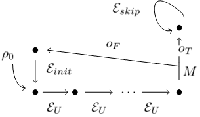
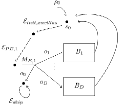
   The first class applies a sequence of unitary operators followed by a measurement. If the outcome of measurement is desirable, the algorithm terminates. Otherwise, the algorithm is re-initialized and executed again; see Figure 1. Examples include the famous quantum order-finding and factoring algorithms [25], the Grover search algorithm [15], several quantum-walk-based algorithms [34, 9, 20] and the algorithm for solving the expectation value of some operators of systems of linear equations [18].

2. 2.

   The second class repeatedly applies an action-measurement loop until success; see Figure 1. One example is the routing algorithm based on a many-measurement quantum walk in [20].

3. 3.

   The structure of the third class looks like a decision tree; see Figure 2. Examples are quantum teleportation [25], one-way quantum computer [29]. These examples always terminate.

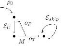
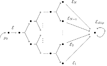
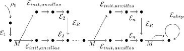
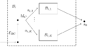
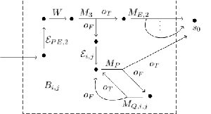
Recently, several algorithms have been developed with the structures different from Figures 1 and 2. For example, a modified quantum factoring algorithm was experimentally realised in [23], where in order to reduce the number of necessary entangled qubits, the ancilla (control) qubits are recycled. The structure of this algorithm is shown in Figure 3. Another example is the quantum Metropolis sampling [36]. This algorithm can be used to prepare the ground or thermal state of a quantum system. The structure of this algorithm for reaching the ground state is shown in Figure 4. It consists of decisions dependent on the history of actions and measurement outcomes as well as repeated loops until success.

As indicated by Figures 1-4, all of the algorithms and protocols mentioned above can be seen as qMDPs. Here we only elaborate the qMDP model of quantum Metropolis sampling.

Various generalisations and variants of quantum Metropolis sampling have been proposed, e.g. quantum rejection sampling [27], quantum-quantum Metropolis sampling [44] and complementing quantum Metropolis algorithm [30]. An experiment for preparing thermal states was realised [45] by employing some ideas from quantum Metropolis sampling. The correctness of quantum Metropolis algorithm and its variants can actually be seen as a reachability problem for qMDPs. This motivates us to systematically develop techniques for reachability analysis of qMDPs.

As one more example of qMDP, we consider a simple concurrent quantum program consisting of $n$ processes. Every process is a quantum loop. We assume a yes/no measurement $M=\{P_{0},P_{1}\}$ in the state Hilbert space $\mathcal{H}$, which is projective; that is, both $P_{0}$ and $P_{1}$ are projections. For each $1\leq i\leq n$, the $i$th process behaves as follows: it performs the measurement $M$, if the outcome is $0$, then it executes a unitary transformation $U_{i}$ and enter the loop again; if the outcome is $1$ then it terminates. Note that the loop guard (termination condition) of the $n$ processes are the same, but their loop bodies, namely unitary transformations $U_{i}$, are different.

This concurrent quantum program can be modelled as a qMDP ${\mathcal{M}}$ with $Act=\{1,2,...,n\}$. For each $i\in Act$, the action super-operator ${\mathcal{E}}_{i}$ is defined by

for all density matrices $\rho$. If $P_{1}$ is the projection onto the subspace $B$ of $\mathcal{H}$, then the overall termination probability of the concurrent program with initial state $\rho$ is the supremum reachability $\Pr\nolimits^{\sup}(\rho\vDash\Diamond B).$ The following proposition provides us with a method for computing this termination probability. We write $\bar{{\mathcal{E}}}$ for the average super-operator of ${\mathcal{E}}_{i}$ ($1\leq i\leq n$); that is,

We further define

(It was shown in [41] that ${\mathcal{E}}_{\infty}$ can be computed by Jordan decomposition of the matrix representation of $\bar{{\mathcal{E}}}$.)

We first examine the case of finite-horizon and consider the following:

Now let us consider a qualitative variant of Problem 3.1.

The counterpart of Problem 3.2.2 for classical MDPs can be stated as follows: given a MDP ${\mathcal{M}}$ with a finite set $S$ of states, an initial state $s_{0}$ and $B\subseteq S$, decide whether there exists a scheduler ${\mathfrak{S}}$ and an integer $N$ such that for any possible sequence of states $s_{0}s_{1}s_{2}\cdots$ under ${\mathfrak{S}}$, there exists $j<N$ such that $s_{j}\in B$. The polynomial-time decidability of this problem immediately follows the fact that an optimal scheduler for maximum reachability problem of a MDP can be found in polynomial time [2]. The only thing we need to do is to check whether there exists a cycle in all states reachable from $s_{0}$ in $S\backslash B$, if $\Pr(s_{0}\vDash\Diamond B)=1$. The same result is true for the counterpart of Problem 3.2.1 for classical MDPs. This idea also applies to partially observable MDPs with a technique for reducing them to MDPs [1].

However, undecidability of Problem 3.2 was proved in [4] if subspace $B$ is allowed to be not invariant. We prove undecidability of the problem for invariant subspace $B$ and thus significantly improve the main result of [4].

Let us turn to the case of infinite-horizon. If the target subspace $B$ is allowed to be not an invariant subspace, then the limit in equation (2) does not necessarily exists, and we consider the corresponding upper limit:

In the remainder of this section, we only consider invariant subspace $B$ of ${\mathcal{M}}$, since the supremum reachability probability is not well-defined for those subspaces that are not invariant (see Definition 2.4 and Lemma 2.1). As for classical MDPs, a major reachability problem for qMDPs is the following:

For a special class of super-operators and measurements operators, Theorem 3.4.1 can be significantly improved:

A variant of Problem 3.3 is the following:

The difference between this problem and Problem 3.3 is that the initial state is arbitrary in the former but it is fixed in the latter. It is worth noting that the counterparts of these two problems for classical MDPs are similar because they have only a finite number of states which can be checked one by one. However, the quantum versions are very different due to the fact that the state Hilbert space of a qMDP is a continuum. It is also worth carefully comparing this problem with Problem 2.1: scheduler ${\mathfrak{S}}$ is given in the latter, whereas we want to find a special scheduler ${\mathfrak{S}}$ in the former.

Based on the above theorem, we develop Algorithm 1 for checking existence of the optimal scheduler, of which the correctness and complexity are presented in the next theorem.

We now consider another variant of Problem 3.3, where not only the initial state $\rho$ but also the scheduler ${\mathfrak{S}}$ can be arbitrary.

For this problem, we only have an answer in a special case.

We can develop an algorithm to check whether $\Pr\nolimits^{\mathfrak{S}}(\rho\vDash\Diamond B)=1$ holds for all initial states and all schedulers ${\mathfrak{S}}$. By Theorem 3.8, we only need to examine all schedulers of the form ${\mathfrak{S}}=s^{\omega}$ with $|s|\leq L_{d}$. There are totally $K_{d}$ such schedulers, and for each one, it costs at most $O(d^{6}L_{d})$ arithmetic operations to check the conclusion. Thus, the complexity of the algorithm is $O(d^{6}L_{d}K_{d})$. For the special class of qMDPs considered in Theorem 3.5, we can significantly reduce this complexity.

To conclude this section, we point out a link from Problems 3.4 and 3.5 to a long-standing problem in matrix analysis and control theory, namely the joint spectral radius problem [16, 37, 8]. For a given set of square matrices $\Sigma=\{A_{i}:i=1,\cdots,t\}$, the discrete linear inclusion of $\Sigma$ is defined to be the set

The set $\Sigma$ is said to be absolutely asymptotically stable (AAS) if $\lim_{n\rightarrow\infty}A_{s_{n}}\cdots A_{s_{1}}=0$ for any infinite sequences $A_{s_{1}}A_{s_{2}}...$ in $\Sigma$. The joint spectral radius and lower spectral radius of $\Sigma$ are defined as

respectively, where for every $k\geq 1$,

It is known [16, 8] that $\Sigma$ is AAS if and only if the joint spectral radius $\bar{\varrho}(\Sigma)<1$. It was shown in [37] that unless $P=NP$, there are no polynomial-time approximate algorithms for computing $\bar{\varrho}(\Sigma)$. The problem “$\underline{\varrho}(\Sigma)<1$” and “$\bar{\varrho}(\Sigma)\leq 1$” were proved to be undecidable in [37, 5]. However, the problem whether “$\bar{\varrho}(\Sigma)<1$” is decidable is still open although the notion of joint spectral radius was introduced more than fifty years ago [31].

References

- [1] C. Baier, N. Bertrand, and M. Größer. On decision problems for probabilistic Büchi automata. In FOSSACS, pages 287-301, 2008.
- [2] C. Baier and J. Katoen. Principles of model checking. MIT Press, Cambridge, Massachusetts, 2008.
- [3] J. Barry, D. T. Barry, and S. Aaronson. Quamtum POMDPs. arXiv:1406.2858.
- [4] V. D. Blondel, E. Jeandel, P. Koiran, and N. Portier. Decidable and undecidable problems about quantum automata. SIAM J. Comput., 34(6):1464-1473, 2005.
- [5] V. D. Blondel and J. N. Tsitsiklis. The boundedness of all products of a pair of matrices is undecidable. Syst. Control Lett., 41(2):135-140, 2000.
- [6] K. Chatterjee, L. Doyen, and T. A. Henzinger. Qualitative analysis of partially observable Markov decision processes. In MFCS, pages 258-269, 2010.
- [7] K. Chatterjee and H. A. Henzinger. Probabilistic automata on infinite words: decidability and undecidability reults. In ATVA pages 1-16, 2010.
- [8] D. Cheban and C. Mammana. Absolute asymptotic stability of discrete linear inclusions. Bul. Acad. Stiine Repub. Mold. Mat., 1: 43-68, 2005.
- [9] A. M. Childs, R. Cleve, E. Deotto, E. Farhi, S. Gutmann, and D. A. Spielman. Exponential algorithmic speedup by a quantum walk. In STOC, pages 59-68, 2003.
- [10] E. D’Hondt and P. Panangaden. Quantum weakest preconditions. Math. Struct. Comp. Sci., 16(03):429-451, 2006.
- [11] S. Gay. Quantum programming languages: survey and bibliography. Math. Struct. Comp. Sci., 16(04):581-600, 2006.
- [12] H. Gimbert and Y. Oualhadj. Probabilistic automata on finite words: decidabale and undecidable problems. In ICALP, pages 527-538, 2010.
- [13] A. D. Gordon, T. Graepel, N. Rolland, C. Russo, J. Borgstrom and J. Guiver. Tabular: a schema-driven probabilistic programming language. In POPL, pages 321-334, 2014.
- [14] A. S. Green, P. LeFanu Lumsdaine, N. J. Ross, P. Selinger and B. Valiron. Quipper: a scalable quantum programming language. In PLDI, pages 333-342, 2013.
- [15] L. K. Grover. A fast quantum mechanical algorithm for database search. In STOC, pages 212-219, 1996.
- [16] L. Gurvits. Stability of discrete linear inclusion. Linear Algebra Appl., 231:43-60, 1995.
- [17] V. Halava. Decidable and undecidable problems in martix theory. TUCS Technical Report No 127, Turku Centre for Computer Science, 1997.
- [18] A. W. Harrow, A. Hassidim, and S. Lloyd. Quantum algorithm for linear systems of equations. Phys. Rev. Lett., 103:150502, 2009.
- [19] M. Hirvensalo. Various aspects of finite quantum automata. In DLT, pages 21-33, 2008.
- [20] J. Kempe. Discrete quantum walks hit exponentially faster. Probab. Theory Relat. Fields, 133(2):215-235, 2005.
- [21] E. H. Knill. Conventions for quantum pseudocode. Technical Report LAUR-96-2724, Los Alamos National Laboratory, 1996.
- [22] S. Lloyd, M. Mohseni and P. Rebentrost. Quantum algorithms for supervised and unsupervised machine learning. arXiv:1307.0411.
- [23] E. Martín-López, A. Laing, T. Lawson, R. Alvarez, X. Zhou, and J. L. O’Brien. Experimental realization of Shor’s quantum factoring algorithm using qubit recycling. Nat. Photon., 6:773-776, 2012.
- [24] D. Monniaux. Abstract interpretation of programs as Markov decision processes. Sci. Comput. Program., 58(1-2):179-205, 2005.
- [25] M. A. Nielsen and I. L. Chuang. Quantum compution and quantum information. Cambridge University Press, Cambridge, 2000.
- [26] B. Ömer. Structural quantum programming. Ph.D. Thesis, Technical University of Vienna, 2003.
- [27] M. Ozols, M. Roetteler, and J. Roland. Quantum rejection sampling. In ITCS, pages 290-308. 2012.
- [28] C. H. Papadimitiou, and J. N. Tsitsiklis. The complexity of Markov decision processes. Math. Oper. Res., 12(3):441-450, 1987.
- [29] R. Raussendorf and H. J. Briegel. A one-way quantum computer. Phys. Rev. Lett., 86:5188, 2010.
- [30] A. Riera, C. Gogolin, and J. Eisert. Thermalization in nature and on a quantum computer. Phys. Rev. Lett., 108:080402, 2012.
- [31] G. C. Rota and W. G. Strang. A note on the joint spectral radius. Indag. Math., 22(4):379-381, 1960.
- [32] J. W. Sanders and P. Zuliani. Quantum programming. In MPC, pages 88-99. 2000.
- [33] P. Selinger. Towards a quantum programming language. Math. Struct. Comp. Sci., 14(4):527-586, 2004
- [34] N. Shenvi, J. Kempe, and K. B. Whaley. Quantum random-walk search algorithm. Phys. Rev. A, 67: 052307, 2003.
- [35] L. J. Stockmeyer and A. K. Chandra. Provably difficult combinatorial games. SIAM J. Comput., 8(2):151-174, 1979.
- [36] K. Temme, T. J. Osborne, K. G. Vollbrecht, D. Poulin, and F. Verstraete. Quantum Metropolis sampling. Nature, 471:87-90, 2011.
- [37] J. N. Tsitsiklis and V. D. Blondel. The Lyapunov exponent and joint spectral radius of pars of matrices are hard – when not impossible – to compute and to approximate. Math. Control Signals Systems, 10(1):31-40, 1997.
- [38] L. M. K. Vandersypen, M. Steffen, G. Breyta, C. S. Yannoni, M. H. Sherwood, and I. L. Chuang. Experimental realization of Shor’s quantum factoring algorithm using nuclear magnetic resonance. Nature, 414:883-887, 2001.
- [39] M. Y. Vardi. Automatic verification of probabilistic concurrent finite state programs. In FOCS, pages 327-338, 1985.
- [40] M. S. Ying. Floyd-Hoare logic for quantum programs. TOPLAS, 33(6): article No. 19, 2011.
- [41] M. S. Ying, N. K. Yu, Y. Feng, and R. Y. Duan. Verification of quantum programs. Sci. Comput. Program., 78(9):1679-1700, 2013.
- [42] S. G. Ying, Y. Feng, N. K. Yu, and M. S. Ying. Reachability probabilities of quantum Markov chains. In CONCUR, pages 334-348, 2013.
- [43] N. K. Yu and M. S. Ying. Reachability and termination analysis of concurrent quantum programs. In CONCUR, pages 69-83, 2012.
- [44] M. H. Yung and A. Aspuru-Guzik. A quantum-quantum Metropolis algorithm. Proc. Natl. Acad. Sci. USA, 109:754-759, 2012.
- [45] J. Zhang, M. H. Yung, R. Laflamme, A. Aspuru-Guzik, and J. Baugh. Digital quantum simulation of the statiscal mechanics of a frustrated magnet. Nat. Commun., 3: Article No. 880.
- [46] P. Zuliani. Nondeterministic quantum programming. In: Proceedings of the 2nd International Workshop on Quantum Programming Languages (QPL), pages 179-195, 2004.