Bilinear Mixed-Effects Models for Affiliation Networks
Yanan Jia¹¹ 1 Department of Statistics, The Ohio State University, Columbus, OH, USA      Catherine A. Calder¹¹ 1 Department of Statistics, The Ohio State University, Columbus, OH, USA³³ 3 Email: calder@stat.osu.edu      Christopher R. Browning ²² 2 Department of Sociology, The Ohio State University, Columbus, OH, USA        

Generally, an affiliation network can be denoted by an $n^{a}\times n^{e}$ affiliation matrix $\mathbf{Y}=\{y_{ik}\}$, which records the affiliation of each actor with each event, where rows index actors and columns index events, and $n^{a}$ and $n^{e}$ are the total number of actors and events, respectively. The entries of this matrix, $y_{ik}$, can be binary variables or non-negative integer-valued variables. If actor $i$ is affiliated with event $k$, then $y_{ik}\geq 1$ and $y_{ik}=0$ otherwise, where $i=1,2,\dots,n^{a}$ and $k=1,2,\dots,n^{e}$. Each row of $\mathbf{Y}$ describes an actor’s affiliation with the events. Similarly, each column of $\mathbf{Y}$ describes the membership of an event. An affiliation network can also be represented by a bipartite graph, or a graph in which the nodes can be partitioned into two subsets corresponding to the distinct modes, and all lines are between pairs of nodes belonging to the different modes. For affiliation networks, since actors are affiliated with events, and events have actors as members, all lines in the bipartite graph are between nodes representing actors and nodes representing events.

Statistical methods for one-mode networks are fairly well developed. The exponential random graph model (ERGM) is one of the most popular methods for analyzing networks (Frank and Strauss,, 1986; Wasserman and Pattison,, 1996; Pattison and Wasserman,, 1999; Robins et al.,, 1999). Although ERGMs are useful for modeling global network characteristics, they are known to possess some undesirable properties. Robins et al., (1999) and Handcock et al., (2003) discussed these challenges associated with ERGMs, including the intractability of the normalizing constant in the likelihood function of ERGMs and model degeneracy. Snijders et al., (2006) proposes an alternative specification of ERGMs that partially addresses these issues, but requires specifying values of tuning parameters. As an alternative, models built on latent variables have attracted considerable attention recently. These models include mixed-effects models (van Duijn et al.,, 2009; Zijlstra et al.,, 2009; Hoff,, 2003; Hoff,, 2005; Hoff,, 2009), the stochastic blockmodel (Wang and Wong,, 1987; Snijders and Nowicki,, 1997; Snijders,, 2001), and latent space models (Hoff et al.,, 2002). All of these latent variable models assume conditional independence of the probability of ties between dyads. That is, the elements of $\mathbf{Y}$ are independent conditional on latent variables. Conditional independence does not imply that latent variable models cannot capture network dependencies of interest. Indeed, some of the more sophisticated latent variable models make clever use of latent structures to capture types of dependence. The conditional independence of edges implies that model degeneracy is not an issue. In addition, the conditional independence of tie probabilities leads to computational advantages in model fitting (Hunter et al.,, 2012). A latent variable model that we build on in this paper is the bilinear mixed-effects model proposed by Hoff, (2005), which is an extension of latent space models for one-mode networks. This model uses interacting latent variables to capture certain types of higher-order dependence patterns often present in social networks.

While there is a rich literature on statistical methods for one-mode networks, methods for two-mode networks are limited. One approach, known as the “conversion,” or projection method (Newman,, 2001), relies on the two one-mode networks that can be derived from an affiliation network: $\mathbf{YY}^{\prime}$ is the one-mode network for actors and $\mathbf{Y}^{\prime}\mathbf{Y}$ is the one-mode network for events. Information is lost, however, by converting an affiliation network into two one-mode networks. For instance, if we use binary matrices to represent the one-mode networks, then we lose information about both the number and the properties of the shared partners of the other set. Alternatively, we can build models for two-mode networks to analyze both actors and events simultaneously. Wang et al., (2009) extended ERGMs to the two-mode situation. However, these models suffer from the limitation of the one-mode ERGMs described above. In addition, they do not readily permit the modeler to investigate patterns in activity participation across multiple events (e.g., whether certain individuals share activity profiles). As we will illustrate, the latent variable approach we take is much more amenable to this sort of study.

Network data differ from other types of dependent data in that ties often tend to be transitive, balanced, and clusterable (Wasserman and Faust,, 1994). In one-mode friendship networks, we often see patterns that indicate “a friend of a friend is a friend,” a statement that translates to properties of sets of three dyads (triangles). In particular, this pattern is called transitivity. Balance is a generalized version of transitivity defined for signed relationship of the type $A_{ij}$ is positive if there is a tie between nodes $i$ and $j$ and is negative otherwise. Formally, a signed relationship between nodes is denoted as follows:

In one-mode networks, a triangle formed by a triad of units $i,j,k$ is said to be balanced if $A_{ij}\times A_{jk}\times A_{ki}>0$. Clusterability is a generalization of the concept of balance. A triangle is clusterable if it is either balanced or the pairwise relationships within the triad are all negative.

Here we extend these definitions to the two-mode setting, which to the best of our knowledge has not been done previously. We say a set of four possible ties among a tetrad of units consisting of one pair of actors $i,j$ and one pair of events $k,l$, $\{A_{ik},A_{il},A_{jk},A_{jl}\}$, forms a cycle, and offer the following definitions.

Transitivity implies that if actors $i$ and $j$ both have a tie with event $k$ and actor $i$ is tied with another event $l$, then we expect actor $j$ also has a tie with event $l$.

Since the number of elements in a cycle is an even number (4), we note that balance and clusterability are identical conceptually in the two-mode setting.

For general signed relations among units, many theories of social systems suggest that the relationships within a cycle tend to be balanced. For example, if $A_{ik}=1$ and $A_{jk}=1$, which means the relationships between actor $i$ and event $k$ and between actor $j$ and event $k$ are positive, then it is more likely that either both $A_{il}=1$ and $A_{jl}=1$ or both $A_{il}=-1$ and $A_{jl}=-1$. In other words, if actors $i$ and $j$ both participate in event $k$, then they are likely to either both participate in event $l$ or both not participate in event $l$. In real affiliation networks, we expect to see more evidence of balance than we would expect if the presence of ties is completely random. This translates into the presence of particular balanced patterns among cycles, which are illustrated in Figure 1.

These configurations, $0$-two-path $(0$-$L_{2})$, $1$-two-path $(1$-$L_{2})$, actor $1$-two-path $(1$-$L_{A2})$, event $1$-two-path $(1$-$L_{E2})$, and four-cycles $(C_{4})$, shown in Figure 1 are the balanced cycles often seen in affiliation networks. Generalizations of these structures, the actor $k$-two-path $(k$-$L_{A2})$ and the event $k$-two-path $(k$-$L_{E2})$, are used by Wang et al., (2009) to define ERGMs for two-mode networks.

Consider the case where actor-event ties within an affiliation network are assumed to be independent and identically distributed with tie probability $\pi_{0}$. In this case, it can be shown that the expected proportion of balanced cycles is $\pi=\pi_{0}^{4}+(1-\pi_{0})^{4}+6\pi_{0}^{2}(1-\pi_{0})^{2}$. In many real networks, the observed proportion of balanced cycles is greater than this theoretical value from this model (i.e., independent and identically distributed ties). That is, $p>p_{0}^{4}+(1-p_{0})^{4}+6p_{0}^{2}(1-p_{0})^{2}$, where $p$ is the observed proportion of balanced cycles and $\pi_{0}$ is the observed proportion of actor-event pairs that are tied. From this, we can see the importance of capturing fourth-order dependence (dependence between tetrads) in models for affiliation network data.

Our data consist of an $n^{a}\times n^{e}$ sociomatrix $\mathbf{Y}$, with entries $y_{ik}$ denoting the value of the relation between actor $i$ and event $k$ and additional covariate information associated with actors, events, and dyads.

In order to capture more transitivity and balance than the generalized linear mixed effects model allows, we add a bilinear random effect to the model given by (3). As with Hoff, (2005)’s bilinear mixed effects model for one-mode network data, this addition enables us to capture the expected balanced tendencies in two-mode network relations.

We presume the existence of a latent social space of dimension $t$. Both actors and events have positions in this latent space, denoted by the vectors $\mathbf{u}_{i}$ and $\mathbf{v}_{k}$, respectively. If we consider the pair of actors with position vectors $(\mathbf{u}_{i},\mathbf{u}_{j})$ (or the pair of events with position vectors $(\mathbf{v}_{k},\mathbf{v}_{l})$), and they have similar direction and magnitude, then the inner products $\mathbf{u}_{i}^{\prime}\mathbf{v}_{k}$ and $\mathbf{u}_{j}^{\prime}\mathbf{v}_{k}$ (or $\mathbf{u}_{i}^{\prime}\mathbf{v}_{k}$ and $\mathbf{u}_{i}^{\prime}\mathbf{v}_{l}$ ) will not be too different. A probability measure over these unobserved characteristics induces a model in which the presence of a tie between an actor and an event is dependent on the presence of other ties. Relations modeled as such are probabilistically balanced.

We add this inner product of latent vectors $\mathbf{u}_{i}$ and $\mathbf{v}_{k}$ to (3) so that

where the random effects $a_{i},e_{k}$ and $\gamma_{ik}$ are still taken to be multivariate normal with means and covariances are as given in Section 2.3.2. This set of bilinear terms $\{\varepsilon_{ik}=\mathbf{u}_{i}^{\prime}\mathbf{v}_{k},i=1,\dots,n^{a},k=1,\dots,n^{e}\}$ allows us to capture balance. To see this further, consider the case in which $t=1$, where $t$ is the dimension of the $\mathbf{u}_{i}$ and $\mathbf{v}_{k}$ vectors. In this case, the $\varepsilon_{ik}$s correspond to the residuals from the version of the model without the bilinear term. Since $\varepsilon_{ik}\times\varepsilon_{il}\times\varepsilon_{jk}\times\varepsilon_{jl}=(u_{i}u_{j}v_{k}v_{l})^{2}\geq 0$, the bilinear term can be seen to capture positive residual cycles. Of course in a real dataset, we do not expect networks to be completely balanced. By taking $t>1$, the bilinear term captures the balanced tendencies of real networks without forcing every residual cycle to be positive.

We assume the $\mathbf{u}_{i}$s and $\mathbf{v}_{k}$s are mutually independent and follow $t$-dimensional multivariate normal distributions so that

In addition, we assume $\mathbf{u}_{i}\perp\mathbf{u}_{j}$ for $\{i,j=1,\dots,n^{a}:i\neq j\}$ and $\mathbf{v}_{k}\perp\mathbf{v}_{l}$ for $\{k,l=1,\dots,n^{e}:k\neq l\}$. It follows that $\varepsilon_{ik}$s have moments

The other second, third, and fourth order moments are all equal to zero. For simplicity, we assume $\boldsymbol{\Sigma}_{u}=\sigma_{u}^{2}\mathbf{I}_{t\times t},\hskip 5.69054pt\boldsymbol{\Sigma}_{v}={\sigma}_{v}^{2}\mathbf{I}_{t\times t}$. In this case, the moments of bilinear term become

This gives the following nonzero second and forth order moments for the bilinear random-effects components, $\epsilon_{ik}=a_{i}+e_{k}+\gamma_{ik}+\mathbf{u}_{i}^{\prime}\mathbf{v}_{k}$:

The bilinear effect $\varepsilon_{ik}=\mathbf{u}_{i}^{\prime}\mathbf{v}_{k}$ can be interpreted as a mean-zero random effect that is able to capture particular fourth order dependence in affiliation network data.

The parameters we want to estimate are $\{\boldsymbol{\beta}_{d},\boldsymbol{\beta}_{a},\boldsymbol{\beta}_{e},{\sigma}_{a}^{2},{\sigma}_{e}^{2},{\sigma}_{\gamma}^{2},{\sigma}_{u}^{2},{\sigma}_{v}^{2}\}$. Following Hoff, (2005), we work with the following representation of our model:

where $\mu^{a}_{i}=\boldsymbol{\beta}_{a}^{\prime}\mathbf{x}_{i}^{a}+a_{i}$ and $\mu^{e}_{k}=\boldsymbol{\beta}_{e}^{\prime}\mathbf{x}_{k}^{e}+e_{k}$ can be viewed as actor and event specific effects, respectively. We then define $z_{ik}=\theta_{ik}-\mathbf{u}_{i}^{\prime}\mathbf{v}_{k}=\boldsymbol{\beta}_{d}^{\prime}\mathbf{x}^{d}_{ik}+\mu^{a}_{i}+\mu^{e}_{k}+\gamma_{ik},$ and let $\mathbf{z}=\text{vec}(\mathbf{Z})$, where $\mathbf{Z}$ is the $n^{a}\times n^{e}$ matrix with elements $z_{ik}$ for $i=1,\dots,n^{a}$ and $k=1,\dots,n^{e}$. We take $\boldsymbol{\theta}$ to be the $n^{a}\times n^{e}$ matrix with elements $\theta_{ik}$, and let $\mathbf{u}$ be a $n^{a}\times t$ matrix with rows $\mathbf{u}_{i}$ for $i=1,\dots,n^{a}$ and $\mathbf{v}$ be a $n^{e}\times t$ matrix with rows $\mathbf{v}_{i}$ for $i=1,\dots,n^{e}$. Then we can write

where $\mathbf{X}_{D}$ is the appropriate design matrix constructed using (4) and $\boldsymbol{\gamma}$ is a vector with dimension $n^{\gamma}$ as described in Section 2.3.2. From (5), it is clear that conditional on the $\boldsymbol{\theta}$s, $\mathbf{u}$s and $\mathbf{v}$s, the other parameters can be sampled using a standard Bayesian normal-theory regression approach.

Our general Gibbs sampler given below is similar to Hoff, (2005)’s algorithm, with the exception of the first part of step 1 and all of steps 2 and 3 in the outline below:

1. 1.

   Sample linear effects:
   Sample $\boldsymbol{\beta}_{d},\boldsymbol{\mu}^{a},\boldsymbol{\mu}^{e}|\boldsymbol{\beta}_{a},\boldsymbol{\beta}_{e},{\sigma}^{2}_{a},{\sigma}^{2}_{e},{\sigma}_{\gamma}^{2},\boldsymbol{\theta},\bf{u},\bf{v}$ (linear regression)
   Sample $\boldsymbol{\beta}_{a},\boldsymbol{\beta}_{e}|\boldsymbol{\mu}^{a},\boldsymbol{\mu}^{e},{\sigma}^{2}_{a},{\sigma}^{2}_{e},{\sigma}_{\gamma}^{2}$ (linear regression)
   Sample ${\sigma}_{a}^{2},{\sigma}_{e}^{2}$, and ${\sigma}_{\gamma}^{2}$ from their full conditionals

2. 2.

   Sample bilinear effects:
   For $i=1,\dots,n_{a}$ sample $\mathbf{u}_{i}|\mathbf{u}_{-i},\mathbf{v},\boldsymbol{\theta},\boldsymbol{\beta}_{d},\boldsymbol{\mu}^{a},\boldsymbol{\mu}^{e},{\sigma}_{u}^{2}$ (linear regression )
   For $k=1,\dots,n_{e}$ sample $\mathbf{v}_{k}|\mathbf{v}_{-k},\mathbf{u},\boldsymbol{\theta},\boldsymbol{\beta}_{d},\boldsymbol{\mu}^{a},\boldsymbol{\mu}^{e},{\sigma}_{v}^{2}$ (linear regression )
   Sample ${\sigma}_{u}^{2}$ and ${\sigma}_{v}^{2}$ from their full conditionals

3. 3.

   Update $\boldsymbol{\theta}$: For actor $i$ and event $k$
   Propose $\theta_{ik}^{*}\sim$ N$(\bm{\beta}^{\prime}X_{ik}+\mu^{a}_{i}+\mu^{e}_{k}+\mathbf{u}_{i}^{\prime}\mathbf{v}_{k},{\sigma}_{\gamma}^{2})$
   Accept $\theta_{ik}^{*}$ with probability $\left[{p(y_{ik}|\theta_{ik}^{*})}/{p(y_{ij}|\theta_{ik})}\right]\bigwedge 1$

The full conditional distributions of $\boldsymbol{\beta}_{d},\boldsymbol{\mu}^{a},\boldsymbol{\mu}^{e}$, $\boldsymbol{\beta}_{a},\boldsymbol{\beta}_{e}$, ${\sigma}^{2}_{a},{\sigma}^{2}_{e},{\sigma}^{2}_{\gamma},{\sigma}^{2}_{u},{\sigma}^{2}_{v},\mathbf{u}_{i}$m and $\mathbf{v}_{k}$ are given in Appendix A.

For binary affiliation network cases, we can use the same algorithm as above with $\sigma_{\gamma}^{2}$ set to a fixed value since over-dispersion is not appropriate for generalized linear models for binary responses. We use this algorithm to fit the model to a binary affiliation network dataset in Section 4 with $\sigma_{\gamma}^{2}=1$.

In addition to the parameters, the dimension of the latent bilinear effects, $t$, is unknown. Choice of $t$ will generally depend on the goal of the analysis. If we want to visualize the bilinear terms in order to understand latent structure in an affiliation network, we can simply choose $t=1,\,2$, or $3$. If the goal is prediction, we can examine higher dimensions and compare models using the Deviance Information Criterion (DIC; Spiegelhalter et al.,, 2002a), or perhaps formally include $t$ in the model space and employ a reversible jump MCMC algorithm for model fitting (Green,, 1995). In Section 4, we try different value for $t$ and report the corresponding DIC. Lastly, if we are interested in whether the model captures particular features of the observed network (Wasserman and Faust,, 1994) or in examining particular aspects of lack-of-fit, we can evaluate the model with posterior predictive checks (Besag,, 2001).

The presence of members of different racial and ethnic groups within a social unit is referred as interracial contact. Interracial contact in the educational setting is an important social issue, but extant research primarily focuses on the racial composition of the school as a whole or within a classroom. In high school, however, extracurricular activities play a significant role in students’ school experiences, but contact patterns between races within extracurricular activities have been largely unexplored (Granovetter,, 1986; Clotfelter,, 2002). Schools that are integrated compositionally may not necessarily result in integrated social interactions if students’ social networks are segregated by race/ethnicity. Moody, (2001) finds that schools in which extracurricular activities are integrated by race/ethnicity exhibit lower levels of race/ethnic segregation in friendship networks, suggesting that extracurricular activities play an important role in diversifying the social experiences of youth. Consequently, accurate characterization of segregation patterns in extracurricular activities by race/ethnicity is necessary in order to understand the features of school social structure that shape actual social interactions and friendship formation. In this section, we examine interracial contact in high school extracurricular organizations by applying our proposed bilinear mixed effects model to student extracurricular activity network data.

We consider a binary affiliation network of student participation in extracurricular activities collected by Daniel McFarland as part of his doctoral dissertation at the University of Chicago (McFarland,, 1999). The data is available in NetData R package (Nowak et al.,, 2012). The extracurricular activity data were collected as part of a larger observational study of two high schools that included classroom observations, surveys, school records, and interviews. We use the data from “Magnet” High, an elite magnet school located in an inner-city neighborhood of a large Midwestern metropolitan area, whose actual name is redacted to protect the confidentiality of the study participants. It is an integrated high school with high-ability students from predominantly lower-income households. While heterogeneous in racial background, Magnet High is rather homogeneous in terms of student ability. The extracurricular activity data was collected from information on voluntary participation in clubs and sports in yearbooks. Gender and racial background on students was ascertained based on yearbook photos, coupled with observation and school records.

The full affiliation network data for Magnet High consists of 1295 students and 91 student organizations, in which participation is recorded over three years (1996-1998) along with individual-level attributes of grade, gender, and race. We combine similar clubs together (see Appendix B) and the newly constructed network has $n^{e}=37$ activities (events). We focus on the $n^{a}=905$ students (actors) in grade 8-12 with non-missing race information listed as Hispanic, Asian, black, and white. We only consider network as it exists in 1996 for our analysis. The data used in our analysis is shown in Figure 2. While this data is nearly 20 years old, we are not aware of more recent data of a similar nature nor has this data been studied from the perspective of interracial contact.

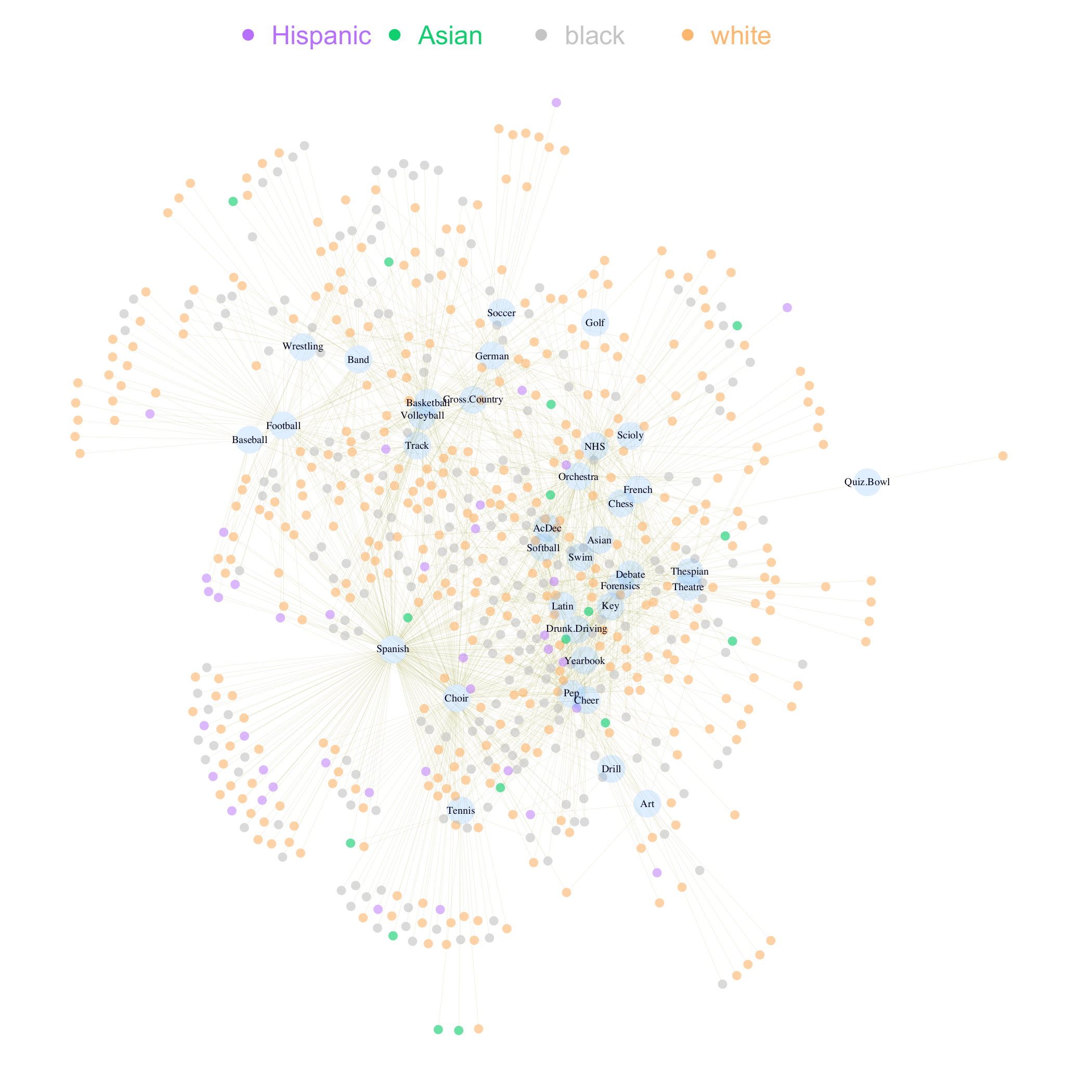
Magnet High is composed of 6 percent Hispanic, 2 percent Asian, 35 percent black, and 57 percent white students. Approximately 72 percent of the students participated in at least one activity. A descriptive plot of activity by race is given in Figure Appendix C.1, and a summary of the data by race is provided in Table 1.

We fit our proposed bilinear mixed-effects models to the extracurricular affiliation network dataset collected from Magnet High. There are no dyad-specific covariates in our analysis, so $\beta_{d}$ corresponds to the intercept. We use gender and race as the actor-specific covariates. Taking “boy” and “white” as the respective base categories for these two categorical covariates, we have actor effect parameters $\beta^{G}_{a}$ (“girl” effect), $\beta_{a}^{B}$ (“black” effect), $\beta_{a}^{A}$ (“Asian” effect), and $\beta_{a}^{H}$ (“Hispanic” effect). Note that these effects are interpreted relative to the baseline log odds of an activity tie for white boys. The size of the clubs is the event-specific covariate, with corresponding effect parameter $\beta_{e}$. From our inferences about the positioning of students in the latent social space, we examine the degree of interracial contact in high school extracurricular clubs using techniques from point pattern analysis.

Before we fit the bilinear mixed-effect model, we check the balance in the data and examine the dependence patterns as described in Section 2.2. For this affiliation dataset, the fraction of ties between actors and events is $p_{0}=0.0705$ (distribution is highly right skewed) and the proportion of balanced cycles, $p$, is $0.8842$. Under an assumption of independence of the actor/event ties, the expected proportion of positive residual cycles is $p_{0}^{4}+(1-p_{0})^{4}+6p_{0}^{2}(1-p_{0})^{2}=0.7724$. If we randomly generate an ${n^{a}\times n^{e}}$ matrix with 7.05 percent positive values (+1) and 92.95 percent negative values (-1) 100 times, the greatest observed proportion of balanced cycles in the 100 matrices is $0.8697$. Therefore, we conclude that the observed proportion of balanced cycles is significantly greater than expected under independence (p-value $\approx 0$).

Prior distributions for the random effect variances (${\sigma}_{a}^{2}$, ${\sigma}_{e}^{2}$, ${\sigma}_{u}^{2}$, and ${\sigma}_{v}^{2}$) are taken to be independent and distributed as $\text{IG}(1,1)$, where $\text{IG}(a,b)$ denotes the inverse gamma distribution with shape $a>0$ and scale $b>0$. The priors for $\boldsymbol{\beta}$ are normally distributed $\boldsymbol{\beta}\sim\text{MVN}(\mathbf{0},\mathbf{I}_{r\times r}).$ The variance of the prior distribution of $\boldsymbol{\beta}$ is small since we are in the logistic regression setting.

The MCMC algorithm described in Section 3.2 was run for 150,000 iterations for values of $t=0\,\text{(no bilinear term)},1,\,2,\,3,\,4,\,5,\,6,\text{and}\,7$. Trace plots suggest that the Markov chain reaches its stationary distribution well before 100,000 iterations, so we conservatively base our inferences on the last 50,000 iterations. DIC (Spiegelhalter et al.,, 2002b) and alternative DIC (Gelman et al.,, 2004) are used to assess our models. The results corresponding to different values of $t$ are listed in Table 2.

In terms of the DIC criterion, model fit generally improves as the dimension of the bilinear terms’ components increases, and the largest decrease in DIC occurs when $t$ changes from 0 to 1. However, the $\text{DIC}_{alt}$ with half the variance of the deviance as an estimate of the number of free parameters in the model keeps increasing and jumps considerably when $t$ increases from $3$ to $4$. Based on the DIC and $\text{DIC}_{alt}$ and considering our ability to plot in two dimensions, we choose to report inferences on the $t=2$ model.

Table 3 provides the posterior mean and standard deviations for all scalar model parameters when $t=2$. The 95 percent credible intervals of all actor-specific covariate coefficients cover 0, which implies that student extracurricular participation generally does not appear to depend on gender and race. As expected, the relationship between club size and the expected log odds of participation is positive with $E[\boldsymbol{\beta}_{e}|\mathbf{Y}]=0.01$, implying that for every additional member, the odds of a particular individual being in the club increases by one percent (since $e^{0.01}=1.01$).

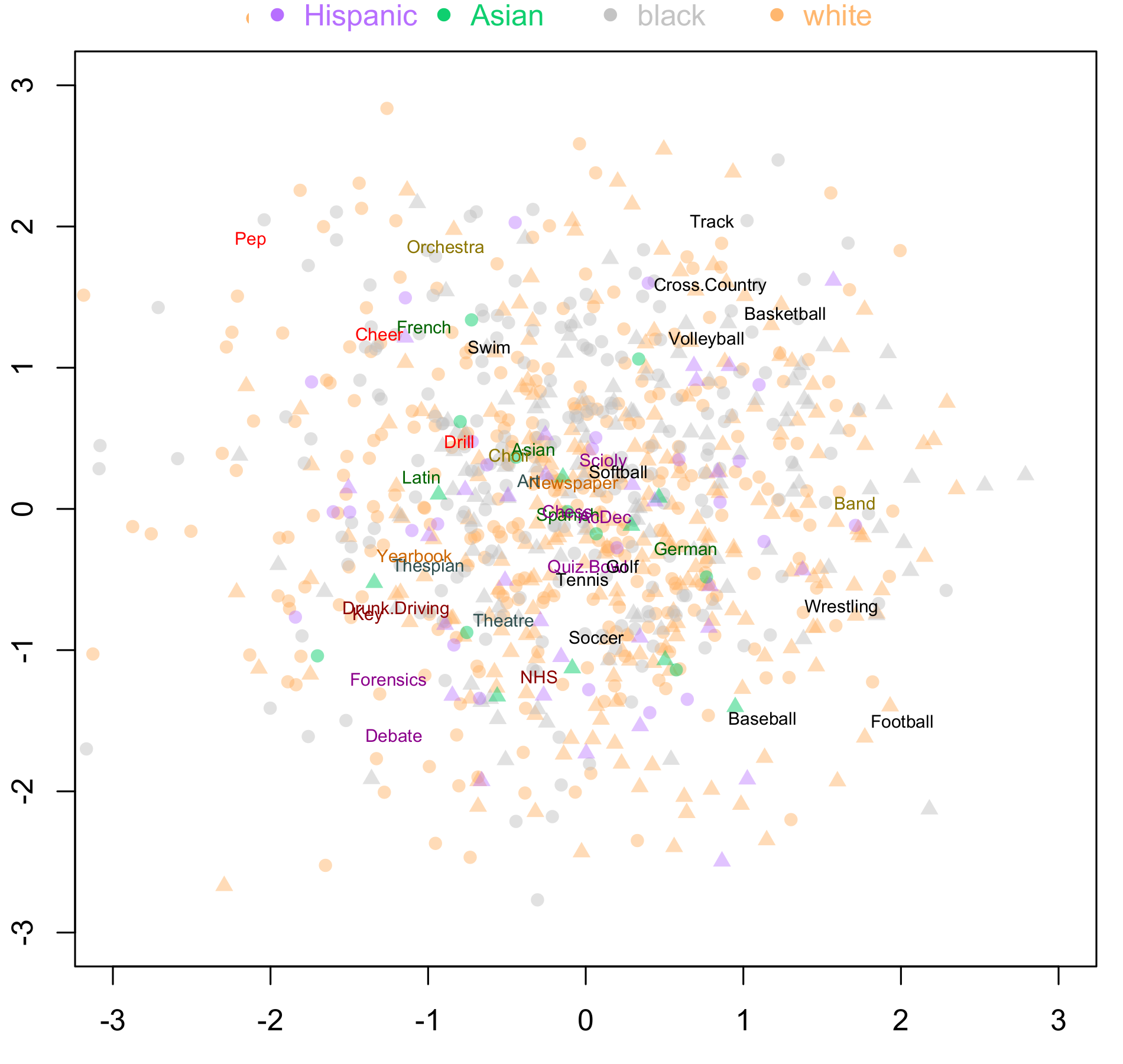
After eliminating the effects of gender, race, and club size on log odds of a student participating in an activity, we explore the structure of the latent social space through the bilinear term, $\mathbf{u}\mathbf{v}^{\prime}$, which captures dependence between the students through common extracurricular activity profiles. First, note that the dimension of the bilinear term $\mathbf{u}\mathbf{v}^{\prime}$ is $n^{a}\times n^{e}$ and that the bilinear model depends on $\mathbf{u}$ and $\mathbf{v}$ only through the inner products $\mathbf{u}\mathbf{v}^{\prime}$, which is invariant under rotations and reflections of $\mathbf{u}$ and $\mathbf{v}$. To appropriately compare posterior samples of $\mathbf{u}$ and $\mathbf{v}$, we first rotate them to a common orientation using a “Procrustean” transformation (Sibson,, 1978) to a Monte Carlo estimate of posterior mean (sample average of the posterior samples), then summarize our inferences by the plot of the posterior mean of $\mathbf{u}$ and $\mathbf{v}$ after rotation which represents the positions of students and activities in the latent social space shown as shown in Figure 3.

The structure of the latent social space can be investigated by examining the position of the activity latent vectors, $\mathbf{v}_{k}$, within this space. To facilitate interpretation in Figure 3, the extracurricular activities are colored based on the assigned categories of activities listed in Appendix B. (Note that these categories were not used in the model fitting.) The positions of students are shown as points in the latent social space. Triangles represent male students, and dots represent female students. The plotting symbol color for the students corresponds race, where white, black, Asian and Hispanic students are colored red, black, yellow, and blue, respectively.

From Figure 3, we can see that generally the activities corresponding in the same category tend to be located nearby each other. For example, we see that Drill, Cheer, and Pep, the three activities in the Cheer category, are located in the upper left capturing the apparent tendency of students to either participate in all or none of these activities. On the other hand, there are examples where the clubs do not cluster based on category. For example, in Music category, Orchestra and Choir locate in the opposite direction from Band indicating a lack of overlap in participants in these groups. From the distribution of the triangles and dots, we see that males dominate the bottom right quadrant of the plot, which makes intuitive sense since the boys-only sports (Football, Baseball, and Wresting) are oriented in this direction. We can also see that girls tend to be more active in the Service, News, and Cheer categories.

To detect patterns of racial segregation within the latent social space, we use techniques from spatial point pattern analysis. Here we consider the students as points in a compact subspace, $D$, defined to be the $6\times 6$ square centered at $(0,0)$ in $\mathbb{R}^{2}$. Each point in $D$ has “mark” defined by the corresponding student’s race. In order to examine racial segregation of students in terms of the extracurricular activity profiles, after controlling for the relative propensity to participate in activities by race and gender, we look for evidence of clustering by race in $D$.

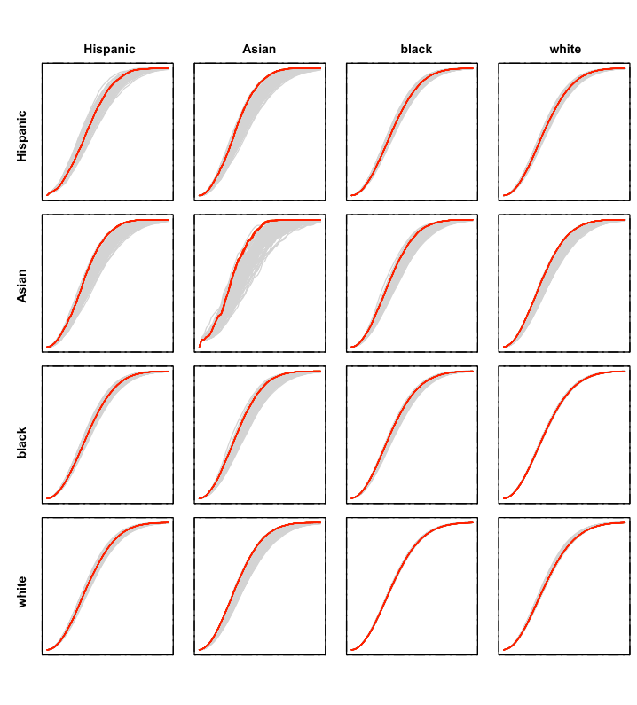
Our investigation of clustering by race is based on Ripley’s multi-type $K$-function (Diggle,, 2003, pages 123-124), where $K_{r_{1}r_{2}}(h)$ is defined as the expected number of students of race $r_{2}$ within a distance $h$ of a typical student of race $r_{1}$, divided by $\lambda_{r_{1}r_{2}}$, where $\lambda_{r_{1}r_{2}}=\lambda_{r_{1}}+\lambda_{r_{2}}$ is sum of the integrated intensity functions of points with marks $r_{1}$ and $r_{2}$ over $D$. For a particular posterior realization, $m$, let $\mathbf{u}^{[m]}_{i}$ denote the position of student $i$ in the latent activity space after rotation. We can estimate $K_{r_{1}r_{2}}(h)$ for this realization as

where $I(\cdot)$ is the indicator function, $r(\cdot)$ returns the race of the student indexed by the function’s argument, $n_{r_{1}}$ and $n_{r_{2}}$ are the number of students of race $r_{1}$ and $r_{2}$, respectively. We can estimate $E[K_{r_{1}r_{2}}(h)|\mathbf{Y}]$ by averaging over the $\hat{K}_{r_{1}r_{2}}^{[m]}(h)$ point-wise over $h$. Alternatively, to get a sense of posterior variability, Figure 4 shows ten posterior multi-type $K$-functions (in red) for each pair of races. (Note that the differences between these red curves is difficult to discern due to the scale of the plots.) For reference, we also recomputed the estimated $\hat{K}^{[m]}_{r_{1}r_{2}}(h)$ under randomization (sampling without replacement) of the race of students with race either $r_{1}$ and $r_{2}$, ten times for each $m$. These estimated multi-type $K$-functions are shown in grey in Figure 4. For all pairs of races, each of the posterior estimated $K$-functions fall within the point-wise as a function of $h$ lower and upper bounds determined by the estimated $K$ functions simulated under randomization, although the Hispanic curves are near the upper bounds. Therefore, we do not find there to be strong evidence of clustering by race within the latent social space determined by extracurricular activity participation. Returning to Figure 2, we can see that in fact the Hispanic students do not appear to be distributed uniformly in this bipartite graphical summary of the data. Our work provides a model-based methodology for formally exploring whether or not students are segregated by race in their extracurricular activity profiles. Lastly, we note that these conclusions are not affected by changing $t$.

References

- Besag, (2001) Besag, J. (2001). Markov chain Monte Carlo for statistical inference. University of Washington, Center for Statistics and the Social Sciences.
- Clotfelter, (2002) Clotfelter, C. T. (2002). “Interracial contact in high school extracurricular activities.” The Urban Review, 34.
- Congdon, (2010) Congdon, P. D. (2010). Applied bayesian hierarchical methods. Chapman & Hall/CRC, Boca Raton, FL.
- Csardi and Nepusz, (2006) Csardi, G. and Nepusz, T. (2006). “The igraph software package for complex network research.” InterJournal, Complex Systems, 1695.
- Davis and Gardner, (1941) Davis, A. and Gardner, B. B. (1941). Deep south. University of Chicago Press, Chicago, IL.
- Diggle, (2003) Diggle, P. J. (2003). Statistical analysis of spatial point patterns. 198 Madison Avenue, New York, NY 10016: Oxford University Press Inc.
- Frank and Strauss, (1986) Frank, O. and Strauss, D. (1986). “Markov graphs.” Journal of the American Statistical Association, 81, 832–842.
- Gelman et al., (2004) Gelman, A., Carlin, J. B., Stern, H. S., and Rubin, D. B. (2004). Bayesian data analysis. New York: Chapman and Hall.
- Granovetter, (1986) Granovetter, M. (1986). “The micro-structure of school desegregation.” In School Desegregation Research: New Directions in Situational Analysis, eds. J. Prager, D. Longshore, and M. Seeman. New York: Plenum Press.
- Green, (1995) Green, P. J. (1995). “Reversible jump Markov chain Monte Carlo computation and Bayesian model determination.” Biometrika, 82, 4, 711–732.
- Handcock et al., (2003) Handcock, M. S., Robins, G., Snijders, T., Moody, J., and Besag, J. (2003). “Assessing degeneracy in statistical models of social networks.” Journal of the American Statistical Association, 76, 33–50.
- Hoff, (2003) Hoff, P. D. (2003). “Random effects models for network data.” In Dynamic Social Network Modeling and Analysis: Workshop Summary and Papers, 303–312.
- Hoff, (2005) — (2005). “Bilinear mixed-effects models for dyadic data.” Journal of the American Statistical Association, 100, 469, 286–295.
- Hoff, (2009) — (2009). “A hierarchical eigenmodel for pooled covariance estimation.” Journal of the Royal Statistical Society, Series B, 71, 971–992.
- Hoff et al., (2002) Hoff, P. D., Raftery, A. E., and Handcock, M. S. (2002). “Latent space approaches to social network analysis.” Journal of the American Statistical Association, 97, 1090–1098.
- Hunter et al., (2012) Hunter, D. R., Krivitsky, P. N., and Schweinberger, M. (2012). “Computational statistical methods for social network models.” Journal of Computational and Graphical Statistics, 21, 856–882.
- McFarland, (1999) McFarland, D. A. (1999). “Organized behavior in social systems: a study of student engagement and resistance in high schools.” Ph.D. thesis, University of Chicago, Chicago, IL.
- Moody, (2001) Moody, J. (2001). “Race, school integration, and friendship segregation in America.” Journal of the Royal Statistical Society, 107, 3, 679–719.
- Newman, (2001) Newman, M. E. J. (2001). “Scientific collaboration networks. I. Network construction and fundamental results.” Physical Review, 64, 016131, 1–8.
- Nowak et al., (2012) Nowak, M., Westwood, S. J., Messing, S., and McFarland, D. (2012). “Network data for McFarland’s SNA R labs.”
- Pattison and Wasserman, (1999) Pattison, P. and Wasserman, S. (1999). “Logit models and logistic regressions for social networks: II. Multivariate relations.” British Journal of Mathematical and Statistical Psychology, 52, 169–193.
- Robins et al., (1999) Robins, G., Pattison, P., and Wasserman, S. (1999). “Logit models and logistic regressions for social networks: III. Valued Relations.” Psychometrika, 64, 371–394.
- Sibson, (1978) Sibson, R. (1978). “Studies in the robustness of multidimensional scaling.” Journal of the Royal Statistical Society, 40, 234–238.
- Snijders, (2001) Snijders, T. A. B. (2001). “The statistical evaluation of social network dynamics.” Sociological Methodology, 31, 361–395.
- Snijders and Nowicki, (1997) Snijders, T. A. B. and Nowicki, K. (1997). “Estimation and prediction for stochastic blockmodels for graphs with latent block structure.” Journal of Classification, 14, 75–100.
- Snijders et al., (2006) Snijders, T. A. B., Pattison, P. E., Robins, G. L., and Handcock, M. S. (2006). “New specifications for for exponential random graph models.” Sociological Methodology, 36, 1, 99–153.
- Spiegelhalter et al., (2002a) Spiegelhalter, D. J., Best, N. G., Carlin, B. P., and Van Der Linde, A. (2002a). “Bayesian measures of model complexity and fit.” Journal of the Royal Statistical Society, Series B, 64, 4, 583–639.
- Spiegelhalter et al., (2002b) Spiegelhalter, D. J., Best, N. G., Carlin, B. P., and van der Linde, A. (2002b). “Bayesian measures of model complexity and fit.” Journal of the Royal Statistical Society, 64.
- van Duijn et al., (2009) van Duijn, M. A., Gile, K. J., and Handcock, M. S. (2009). “A framework for the comparison of maximum pseudo likelihood and maximum likelihood estimation of exponential family random graph models.” Social Networks, 31, 52–62.
- Wang et al., (2009) Wang, P., Sharpe, K., Robins, G. L., and Pattison, P. E. (2009). “Exponential random graph models for affiliation networks.” Social Networks, 31, 12–25.
- Wang and Wong, (1987) Wang, Y. J. and Wong, G. Y. (1987). “Stochastic blockmodels for directed graphs.” Journal of the American Statistical Association, 82, 397, 8–19.
- Wasserman and Faust, (1994) Wasserman, S. and Faust, K. (1994). Social network analysis: methods and applications. Cambrige University Press, Cambrige.
- Wasserman and Pattison, (1996) Wasserman, S. and Pattison, P. (1996). “Logit models and logistic regression for social networks: I. An introduction to Markov graphs and p*.” Psychometrika, 61, 401–425.
- Zijlstra et al., (2009) Zijlstra, B. J. H., van Duijn, M. A. J., and Snijders, T. A. B. (2009). “MCMC estimation for the p2 network regression model with crossed random effects.” British Journal of Mathematical and Statistical Psychology, 62, 143–166.
APPENDICES
Appendix A Full Conditional Distributions
Full conditional distribution of
The full conditional distribution of is proportional to
Assume the prior distribution of follows a multivariate normal distribution
We already know that and . So, we have
where is a matrix, , and .
Since are independent and Gaussian, we can rewrite their joint distribution as
Let so
It follows that the full conditional distribution is multivariate normal with the following mean and covariance:
The full conditional distribution of is proportional to Assume the combined regression parameter has a multivariate normal prior: .
Therefore, the full conditional is a multivariate normal distribution with the following mean and variance:
We restrict and . For , and , the full conditionals are independent and
and
We restrict . Using prior distribution of , the full conditional distribution of is
Let , as before, and . Then ,
Considering the full conditional of , we have
so . Therefore, sampling from its full conditional is equivalent to a Bayesian linear regression problem. Assuming the s are a priori independent and the full conditional of is multivariate normal with
Similar to the derivation of the full conditional distribution of , we have .
. Therefore, sample from its full conditional is also equivalent to a Bayesian linear regression problem. Assuming the s are a priori independent and each . the full conditional of is multivariate normal with
We restrict and and let and . Then the full conditionals are
Appendix B Data Processing
In our analysis of McFarland, (1999)’s data for year 1996, we collapsed several extracurricular activity categories as described below. For example, our club “Pep” includes both members of “Pep.Club” and “Pep.Club.Officers.” In addition, we grouped the activities into one of eight types labeled as 1-8 below. These groups were not used in fitting our model, but were helpful in interpreting our fitted model.
- 1.
Language
- (a)
Asian
- (b)
Spanish includes Hispanic.Club, Spanish.Club, Spanish.Club..high.,Spanish.NHS
- (c)
Latin
- (d)
French includes French.Club..low., French.Club..high., French.NHS
- (e)
German includes German.Club, German.NHS
- 2.
Academic Competition
Debate
Forensics includes Forensics, Forensics..National.Forensics.League.
Chess
Science.Olympiad
Quiz.Bowl
- (f)
Academic.Decathalon
- 3.
News
Newspaper
Yearbook includes Yearbook.Contributors, Yearbook.Staff
- 4.
Cheer
Pep includes Pep.Club, Pep.Club.Officers
Drill
Cheer includes Cheerleaders..8th, Cheerleaders..9th, Cheerleaders..Spirit.Squad, Cheerleaders..JV, Cheerleaders..V
- 5.
Service
National Honor Society
Drunk.Driving includes Drunk.Driving, Drunk.Driving.Officers
Key
- 6.
Art/Theater
Art
Theatre
Thespian
- 7.
Music
Band includes Band..8th, Band..Marching..Symphonic., Band..Jazz
Orchestra includes Orchestra..8th, Orchestra..Full.Concert, Orchestra..Symphonic
Choir includes Choir..treble, Choir..concert, Choir..women.s.ensemble, Choir..a.capella, Choir..chamber.singers, Choir..vocal.ensemble..4.women., Choir..barbershop.quartet..4.men.
- 8.
Sports
Football includes Football..8th, Football..9th, Football..V
Soccer
Volleyball includes Volleyball..8th, Volleyball..9th, Volleyball..JV, Volleyball..V
Basketball includes Basketball..boys.8th, Basketball..boys.9th, Basketball..boys.JV, Basketball..boys.V, Basketball..girls.8th, Basketball..girls.9th, Basketball..girls.JV, Basketball..girls.V
Baseball includes Baseball..JV..10th., Baseball..V
Softball includes Softball..JV..10th., Softball..V
- (g)
Cross.Country includes Cross.Country..boys.8th, Cross.Country..girls.8th , Cross.Country..boys.V, Cross.Country..girls.V
- (h)
Golf
- (i)
Swim includes Swim…Dive.Team..boys, Swim…Dive.Team..girls
- (j)
Tennis includes Tennis..boys.V, Tennis.girls.V
- (k)
Track includes Track..boys.8th, Track..girls.8th, Track..boys.V, Track..girls.V
- (l)
Wrestling includes Wrestling..8th, Wrestling..V
Appendix C Club affiliations by race