Queued cross-bar network models
for replication and coded storage systems
Abstract
Coding techniques may be useful for data center data survivability as well as for reducing traffic congestion. We present a QCN (QCN) method that can be used for traffic analysis of both replication/uncoded and coded storage systems. We develop a framework for generating QCN RR by analyzing their conflict graph stable set polytopes (SSPs). In doing so, we apply recent results from graph theory on the characterization of particular graph SSPs. We characterize the SSP of QCN conflict graphs under a variety of traffic patterns, allowing for their efficient RR computation. For uncoded systems, we show how to compute RR and find rate optimal scheduling algorithms. For coded storage, we develop a RR upper bound, for which we provide an intuitive interpretation. We show that the coded storage RR upper bound is achievable in certain coded systems in which drives store sufficient coded information, as well in certain dynamic coding systems. Numerical illustrations show that coded storage can result in gains in RR volume of approximately 50%, averaged across traffic patterns.
I Introduction
The continued growth in DC (DC) demand worldwide is driving the development of new DC architectures and data management techniques. Two key parameters of data management in DC are the survivability of data in the event of node failures and constant availability of data. Significant academic literature has focused on data survivability in the form of regenerating codes. See [1] and references therein. In enterprise-level DC temporary drive unavailability dominates permanent failure by a factor of nine to one [2]. In this paper we concentrate on data unavailability due to traffic congestion.
We consider physical storage networks as illustrated in Fig. 1. Chunks are fixed-size file subsets. A network of drives, where each drive is either a HDD (HDD), SSD (SSD), or RAM cache, stores some number of file chunks. Outside users send read requests for file chunks to the drive network, and drives process read requests and send chunks back to users. Time is slotted and in each timeslot the network is constrained as to how many users each drive can transmit a stored chunk to; we refer to these constraints as traffic patterns.

To the author’s knowledge, the following key questions are unaddressed when designing and implementing high-traffic storage networks: What is the maximum achievable rate of a storage network with general traffic patterns and arbitrary chunk-to-drive mappings? There do not exist systematic methods of mapping physical networks to queueing models. What is the impact of coded storage on the maximum achievable rate of a storage network? Existing queueing work on coded storage either assumes perfect scheduling or uses scheduling heuristics. Further, what scheduling algorithms achieve maximum rate for coded storage?
Referring to Fig. 2, the main contributions of this paper are as follows.
- •
We introduce the QCN (QCN) method, which is a technique to model relatively general physical drive networks as queueing networks. Our technique allows for arbitrary traffic patterns as well as chunk-to-drive mappings.
- •
To determine the effect of drive traffic pattern restrictions, we develop a framework for analyzing QCN RR by considering their conflict graph stable set polytopes (SSPs). In doing so, we use and adapt existing techniques from cross-bar switching literature.
- •
We exactly characterize the SSP of QCN conflict graphs under a variety of traffic patterns, allowing for their efficient RR computation.
- •
For uncoded storage, we characterize RR, and prove that the existing scheduling algorithm of Tassiulas et al. [3] can be modified to be rate optimal in this application. For coded storage, we develop a RR upper bound, for which we provide an intuitive interpretation. We show that the coded storage RR upper bound is achievable in certain coded systems in which drives store sufficient coded information, as well in certain dynamic coding systems.
- •
We present numerical illustrations that show potential increases in RR volume from coded storage, averaging 50% across traffic patterns.
This paper builds upon and complements existing work in coded storage. General scheduling for coded storage in point-to-point networks, when users are served sequentially instead of simultaneously, and with particular file layouts are considered in [4, 5]. Server scheduling is also well studied in matched networks such as cross-bar switches. Throughput-optimal schedules are considered for point-to-point cross-bar switches using graph theory and techniques such as the Birkhoff-von Neumann theorem [6, 7, 8]. Switches with multicast and broadcast capabilities with a queueing analysis flavor are considered in [9]. References [10, 11] attempt to map the multicast problem in cross-bar switches to simpler problems such as block-packing games and round-robin based multicast. Chunk scheduling problems in uncoded peer-to-peer networks, as opposed to PMP, are considered in [12], and for star-based broadcast networks in [13]. This manuscript differs from these works in that we consider general traffic patterns and arbitrary chunk-to-drive mappings. We also consider scheduling for coded storage.
Scheduling for network coded multicast in multihop wireless networks, using a conflict graph approach, is considered in [14]. Reference [15] developed optimal scheduling algorithms for cross-bar switches with network coding in communications. Enhanced conflict graphs, closely related to classical conflict graphs, were developed to allow analysis of cross-bar switches with network coding. The stable sets of these conflict graphs were then characterized exactly by showing that in certain cases they are perfect graphs. Although in general characterizing stable set polytopes is NP-hard, if the conflict graph is claw-free, then it can be done in polynomial time [16, 15]. We use the fact that certain traffic patterns produce graphs whose
I-A Summary of Main Results
All results assume drives with deterministic read times.
- 1.
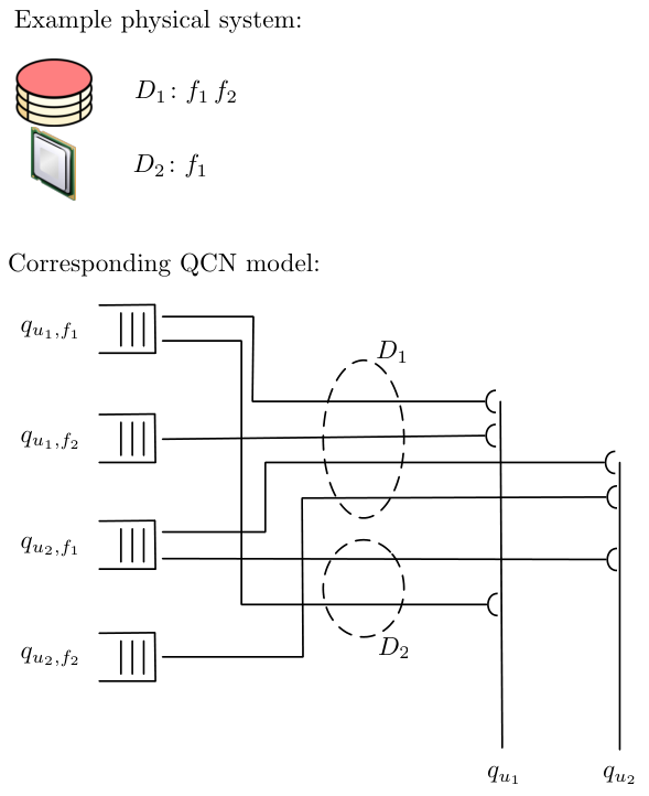
In Sec. IV, we develop a QCN model that can be used to map a storage network with arbitrary file layouts across drives into a queueing network, including systems with nonuniform file or chunk replication. In the spirit of [17], Sec. IV-A describes our QCN model as a moded system, whereby valid modes are described as inequalities that capture multipacket reception, drives with multiple service units, and multiple unicast, broadcast, and multicast traffic or communication patterns. See Fig. 3 for an example.
- 2.
Sec. V-A describes the construction of a conflict graph from the QCN model, in which we divide our analysis into systems in which drives have infinite or finite I/O access bandwidth.
- 3.
Sec. V-B characterizes the stable set polytope for finite I/O bandwidth systems. We show that, for systems under a multicast traffic pattern, associated conflict graphs are not guaranteed to be claw-free. However, systems with a broadcast only as well as broadcast or single unicast traffic patterns result in perfect and claw-free conflict graphs. In a system with sufficient multipacket reception or with a multiple unicast traffic pattern, the conflict graph is a quasi-line graph. We then use recent results [18] that allows the characterization of stable set polytopes for quasi-line graphs, which are a strict superset of perfect graphs. See Table I for a summary.
- 4.
Sec. V-C adopts and adjusts techniques from Tassiulas et al. [3] to transform our conflict graph characterizations into an offline scheduling algorithm that is rate optimal for uncoded storage. For coded storage, Sec. VI develops a RR upper bound, for which we provide an intuitive interpretation, or equivalently the RR given particular dynamic coding systems. The upper bound is found by adding links into an equivalent uncoded QCN model, which intuitively depicts coded storage’s additional initial scheduling options.
Sec. VII then presents examples and numerical results showing that the RR of coded storage can subsume that of uncoded storage, with increases in volume averaging 50% across traffic patterns.
The remainder of this paper is organized as follows. The general system model and basic notation is described in Sec. II. Preliminaries are detailed in Sec. III. The QCN model construction is detailed in Sec. IV and the characterization of associated conflict graphs is presented in Sec. V. Sec. VI discusses the effect of coded storage, and Sec. VII presents examples and numerical results. Finally, Sec. VIII concludes the paper.
II System Model
We study storage systems with the following system model.
- •
File layout: Without loss of generality, consider a single chunked file is stored in drives, and the th drive stores a subset of chunks .11 1 may represent one or more logical physical files. (We do not consider multisets in which single drives can store multiple chunk replicas.) Let the total number of chunks stored in the system be equal to , and .
- •
Drive behavior: Drives have deterministic read and communication pattern of one chunk per timeslot per service unit. (We do not allow preemption or processor sharing between drives.) Drive has service units vis-à-vis queueing theory. We refer to each service unit as a virtual drive, and label the set of virtual drives as , where .
- •
User management: At any given time, the system can manage up to finite active users, denoted by . These users can be, for instance, subscribers to a system or connected routers or other aggregating nodes in a larger content distribution network.
- •
Server behavior: As in classic PMP (PMP) networks [19], we consider servers that can multicast chunks read from drives to user subsets with various structures, including a multicast traffic pattern.
Consider a queueing network composed of a set of input queues or buffers , each of potentially infinite size, and a set of output lines or sinks connecting to outside users. Outside users send read request for file chunks to the network, and requests arrive at . When a read request is serviced, appropriate chunks are read from one or more drives, and that read data is then transmitted to a set of users using output lines in . We say that a read request has been serviced when that request has left its input queue, the requested chunk has been read from drives and then completed transmission on all appropriate output lines.
All lines have the same capacity called the line rate. All virtual drives have the same deterministic capacity and read-times. Time is slotted, where the length of a timeslot is the reciprocal of the line rate plus the read time of a service unit.
III Preliminaries
This section will introduce select topics in queueing and graph theory used later in the paper. It will also introduce the reader to the communications or traffic patterns that are considered throughout the paper. Again, refer to Fig. 2 for an illustration of the method used in this paper. Readers fluent in both queueing and graph theory are encouraged to immediately read Sec. IV and to use this section simply as a reference for notation.
III-A Queueing Theory
This subsection lists preliminary queueing theory definitions used throughout the paper. The reader is referred to [20] for a more thorough survey on queueing theory.
A flow and rate are the stream of all read request chunks, and the average number per timeslot, respectively, that arrive at some input queue that need to be serviced via output lines . Let denote the rate vector of all rates into all input queues.
A set of flows is called admissible if the sum of the rates of all the flows through each input queue or output line does not exceed one, so inputs and outputs are not oversubscribed.
A rate vector is said to be achievable if there exists a schedule that can serve it, while keeping all queues stable.
The rate region is the set of all achievable rate vectors.
III-B Traffic Patterns
We explore various storage, communication, link, and traffic patterns throughout the paper. In PMP (PMP) networks, a number of communication strategies or traffic patterns are possible between the physical drives that read chunks, and the users receiving those chunks, depending on the system technologies. Unless explicitly stated otherwise, all systems are assumed to have single packet reception.22 2 A packet will consist of the read chunk, as well as some overhead as required by the communication protocol. We assume that such overheads are negligible.
A PMP storage system has a particular traffic pattern if, in every timeslot, the set of feasible flows from virtual drives to output lines must meet particular constraints. General traffic patterns are captured by the QCN (QCN) model described in Sec. IV. Specific traffic patterns analyzed in this paper are:
(Single Unicast) A system uses a single unicast traffic pattern if, in every timeslot, a maximum of one output line can be used to service a chunk read by a single virtual drive.
(Multiple Unicast) A system uses a multiple unicast traffic pattern if, in every timeslot, each output line can be used to service a chunk, but chunks transmitted along each output line must be read by distinct virtual drives.
(Broadcast) A system uses a broadcast traffic pattern if, in every timeslot, each output line must transmit the same chunk read by the same virtual drive.
(Multicast) A system uses a multicast traffic pattern if, in every timeslot, each output line can be used to service a single chunk from any virtual drive.
(Multipacket Reception) A system uses -chunk multipacket reception if, in each timeslot, the th output line or channel can be used to transmit unique chunks without error. From a modeling perspective, multipacket reception (MPR) for communications can be viewed as a generalization of speed-up in cross-bar switches [15]. Speed-up is obtained by the communication medium operating at a faster rate, and multipacket reception can be obtained either by speed-up or by particular communication receivers or codes being employed.
III-C Coded Storage
Coded storage allows physical drives to store linear combinations of chunks, as opposed to only individual chunk subsets. We refer the reader to [1] for a survey of codes for distributed storage. We denote the th uncoded chunk as , and the corresponding th coded chunk in the coded system, stored in the same physical location, as . The set of chunks whose information is encoded or mixed with is called the generation of chunk , whose set of uncoded chunk indices we denote by . Chunks, be they coded or not, consume the same storage space (ignoring any overhead for storing coding parameters). In this manuscript, we focus on MDS (MDS) codes, and do not allow the coded chunks to update or regenerate once they are loaded onto physical drives. MDS codes are those in which a set of chunks or a generation is encoded into coded chunks and, if a user downloads any coded chunks, then that full generation can be decoded. We make two key assumptions regarding coding:
- •
No user should receive a replica coded chunk from a generation prior to being able to decode that generation.
- •
If a chunk is coded within any generation, then all replicas of are also coded.
A Reed-Solomon code is an example of an MDS code. During a particular timeslot, a user is said to require additional degrees of freedom if they require unique additional coded chunks from the storage system to decode a particular generation to be able to decode chunks in the associated generation. Further, is said to be innovative for a user if receiving would reduce the required degrees of freedom for that user by one.
III-D Graph Theory
This subsection lists graph theory definitions used throughout the paper. We refer the reader to [16] for a more thorough survey on graph theory. Definitions are across graph , composed of vertices and edges .
(Hyperedge) A hyperedge is of graph is an edge , the power set of . In particular, a hyperedge can connect any number of vertices from that graph, instead of only two vertices.
(Incidence vector) The incidence vector of a set of vertices is a -vector whose entries are labeled with the vertices of . If , then vertex is in ; otherwise, .
(Clique) A subgraph is called a clique if all vertices in the subgraph are pairwise connected.
(Stable set) A set of vertices forms a stable set if for every pair of vertices in , there is no edge connecting the two.
(Stability number) The stability number is the maximum cardinality of a stable set of .
(Stable set polytope) The stable set polytope of a graph is the convex hull of the incidence vectors of the stable sets of .
(Claw-free graph) We say that a conflict graph is claw-free if no induced subgraph of is a vertex with three pairwise disconnected neighbors.
(Quasi-line graph) A graph is a quasi-line graph if the closed neighborhood of every vertex can be partitioned into two cliques.
(Chromatic number) The chromatic number of graph is the smallest number of colors needed to color the vertices of so that no two adjacent vertices share the same color.
(Perfect graph) A graph is perfect if the chromatic number of every induced subgraph equals the size of the largest clique of that subgraph.
III-E Conflict Graphs
Conflict graphs are discussed in detail in [21, 22]. A brief overview follows. Given network graph , and associated feasibility constraints across , conflict graphs allow the visualization of those feasibility constraints. In this paper conflict graphs are between hyperedges in the queueing network model. In general, conflict graph construction generates a simple33 3 A graph is simple if it has no loops or parallel edges. and finite conflict graph as follows:
- •
For every possible hyperedge , create a set of vertices in so that there is a one-to-one correspondence between all possible states of hyperedge (excluding the empty set state ) and the vertices .
- •
Connect vertices and if assigning state to and state to simultaneously is impossible due to a conflict across feasibility constraints [15].
A stable set from the conflict graph represents a collection of links that can operate simultaneously without conflict, hence it represents a valid system mode. The SSP (SSP) can be thought of as the convex combination of all valid modes and through timesharing, any point in the SSP can be set as the system operating point.
General conflict graphs have the potential to have a large number of states and to be computationally intractable. Indeed, for general graphs the problem of solving the maximum stable set problem is known to be NP-hard. If the graph has particular structure such as being claw-free, then the maximum stable set problem can be solved in polynomial time. However, more than 20 years after the discovery of a polynomial algorithm for the maximum stable set problem for claw-free graphs, the explicit description or characterization of the SSP for claw-free graphs remains an open problem [18]. Recently, it was proved that if the conflict graph is a quasi-line graph (a strict subset of claw-free graphs), then the SSP can be characterized exactly using the clique-family inequalities presented in [18]. We use this result in this paper. In addition, note that if the conflict graph is perfect (a strict subset of quasi-line graphs), then the SSP can also be exactly characterized using the techniques summarized by Kim et al. [15].
III-F Generating Rate Regions from Conflict Graphs
For networks composed of buffers, each of potentially infinite size, and without multicast capabilities, it is well known that the rate region is given by
| (1) |
where are the maximum stable sets of the conflict graph, and denotes the non-negative real -vectors [17], where is the total number of input buffers in . This is exactly the SSP of the traffic pattern’s conflict graph. In addition, it has been shown in [23] that in infinite buffer networks with multicast traffic patterns but no fanout-splitting, the RR is again the SSP of the traffic pattern’s conflict graph.
III-G Generating Scheduling Algorithms from Conflict Graphs
We consider the development of offline scheduling algorithms, which require knowledge of the incoming traffic statistics of read requests into . Given a cross-bar switch network, the stable set polytope from its conflict graph, and a particular operating point that is within the stable set polytope, it has been shown that frame-based algorithms, with parameters appropriately chosen, can serve any traffic pattern in the stable set polytope and achieve maximum throughput [15]. A frame is a set of consecutive timeslots, where is the frame size. Frame-based schedules are specified by a sequence of mode schedules and the scheduler cycles through these modes periodically. The authors in [15] generated conflict graphs such that each system queue can be served by a maximum of one vertex, and although this is an assumption we shall generalize, the ideas presented herein will rely heavily on the frame-based offline scheduling from [15].
IV Queued Cross-bar Network Model
This section presents our general queued cross-bar network (QCN) model, which is a queueing model constructed from a physical storage network, as per Sec. II. We generate this queueing network as follows.
- •
For chunk and user , there exists one infinite size input queue labeled . Consider the set of input queues.
- •
For every user we create an output sink , and denote the set of output sinks.
- •
As a reminder of the system model, for each service unit on each physical drive, we create a virtual drive . In the context of the QCN model, when we refer to drives we are always referring to virtual drives.
- •
For any that drive can read, we draw an edge from every queue in , i.e., corresponding to chunk for any user, to output line with label (labels are not necessarily unique).
System connectivity is represented using three matrices. Let chunk-drive connectivity be defined by , a matrix such that each element is defined as
| (2) |
During each timeslot, set the status of each user’s file knowledge through a matrix , such that for a particular timeslot, each element is defined as
The mode set is given as follows. Let be the set of all modes, where is the th mode which is an matrix where each element is defined as
| (3) |
Let chunk-drive usage indicator be defined as,
| (4) |
We call the system the QCN (QCN) model. See Fig. 3 for a simple illustration.
IV-A Constraints
The set of constraints required for mode to be valid are as follows.
- •
A user never receives a non-innovative chunk
(5) - •
Up to chunks can be received by the th user in each timeslot, i.e., user has -chunk multipacket reception capability
(6) - •
The th (virtual) drive allows up to one read per timeslot
(7) - •
Traffic pattern constraints:
- –
Single unicast constraint: Only a single chunk can be transmitted to a single output line
(8) - –
Multiple unicast constraint: Only up to one user can receive a chunk from the same drive
(9) - –
Broadcast constraint: If a read chunk is transmitted from to a user, then it is transmitted to all users
(10) - –
Multicast constraint: Up to users can receive the same chunk from the same drive
(11)
- –
The QCN model incorporates arbitrary chunk layouts, service unit numbers, as well as traffic patterns, which may make it a useful tool in high-traffic storage network analysis. Example systems with the traffic patterns described above are as follows. Some systems may be restricted to multiple unicast traffic patterns if they do not allow caching, others may be restricted to broadcast traffic patterns if they are transmitting wirelessly. Systems can be modeled as having multipacket reception if their scheduling is done at the level of frames, or multiple timeslots if output buffers exist on each output line.
IV-B Properties
To explore the storage system types that the QCN model can capture and model, we introduce the following properties.
(Conservation of flow:) We say that a queueing model has the conservation of flow if in any timeslot, the sum of the number of read requests serviced across input queues is equal to the sum of the number of chunks received at output lines , regardless of traffic pattern constraints.
(Multiple service unit property:) We say that a queueing model has the multiple service unit property, if for any physical drive , up to any fixed unique and stored chunks can be read from physical drive in any timeslot. A queueing model that has both conservation of flow and the multiple service unit property can be used to model a large variety of systems, regardless of chunk-to-drive layouts.
Theorem 1.
Any QCN model has conservation of flow.
Proof.
Any queueing network with fixed topology and in which all service units have deterministic service time has conservation of flow by construction. For a QCN model, in each timeslot a single mode is selected and so we need to check that no mode exists which does not have conservation of flow.
Suppose mode does not have conservation of flow. In this case, either we service more read requests from than are received at , or we transmit more chunks down output lines than are serviced across .
Suppose mode services more read requests than are received by users. This implies there exists output line that receives less chunks than are serviced at queues . implies any valid mode can only activate edges on virtual drives with chunks in demand, and owing to (7), there is either overflow servicing from the same chunk on different virtual drives, or from different chunks from different drives. Suppose it is the same chunk on different virtual drives; if those cross bars are activated then cross bars are activated. The only way for such invalid overflow to occur is if , and by (6) we have a contradiction. The same contradiction holds for different chunks on different virtual drives.
Suppose mode services fewer read requests than are received by users. This implies there exists a queue that transmits a request to more than . However, by construction no such labeled links exist in the QCN model, so we have a contradiction.
∎
Theorem 2.
The QCN model has the multiple service unit property.
Proof.
This follows naturally from the construction of the QCN queueing model from a physical network. If a physical drive has service units, we construct virtual drives, all with access to physical drive ’s chunks. All constraints are indexed across virtual drives in , so the property holds by construction. ∎
V Rate Region Characterization
In this section we generate our conflict graph and then characterize the rate region.
V-A Conflict Graph
Conflict graphs are constructed as follows. We use hyperedges as defined by traffic pattern constraints, so that all data is transmitted along the same fingers of the same hyperedge.
In our conflict graph analysis, we restrict ourselves to edge-based conflict graphs. A conflict graph can be edge-based if ; for -multipacket reception with , then the conflict graph may require hyperedges to capture the selection of different copies of chunks.
Drive I/O access bandwidth—tightly coupled to the number of service units per drive—is a key parameter of modern storage systems. As such, to build up intuition, we begin by analyzing simpler systems with infinite I/O access bandwidth, and then move to finite bandwidth systems. An infinite I/O system model would be helpful when individual drive blocking is not a bottleneck, and instead traffic patterns are the main constraint so wish to analyze their effects directly.
V-A1 Infinite I/O Access Bandwidth
Consider the case when . In this scenario, a drive can read out all chunks simultaneously in a timeslot, so no intra-drive conflicts can arise.
As defined prior, is the set of active users in the system. To simplify the problem and reduce vertex numbers, we define valid conflict graph vertices using the set of valid traffic pattern constraints. The connectivity between these vertices is then set by storage and link constraints.
Vertices: For every chunk stored in the system , we ignore the drive that stores it since each drive has infinite I/O bandwidth. Given a particular conflict graph traffic pattern constraint, we generate a set of vertices in our conflict graph as
- •
Multicast: , where is the powerset of all active users excluding the empty set of users. The total number of vertices in the conflict graph then scales as .
- •
Broadcast: , i.e., a single vertex. The total number of vertices in the conflict graph scales as .
- •
Multiple unicast: , i.e., a set of vertices. The total number of vertices in the conflict graph scales as .
Edges: Consider two vertices generated by the traffic pattern constraints, , and . Given some and such that , if setting
| (12) |
and
| (13) |
violates at least one storage or link constraint as in Sec. IV-A, then connect , and with an edge.
V-A2 Finite I/O Access Bandwidth
Consider the case when .
Vertices: Similarly to the infinite I/O scenario, we generate viable vertices via our traffic pattern constraints. The primary addition is that we generate separate vertices for duplicate chunks stored on other virtual drives.
Given our chunk-drive connectivity matrix , for every non-zero element of we generate a set of vertices in our conflict graph, given by our traffic pattern constraints as:
- •
Multicast: , where is the powerset of all active users excluding the empty set of users. The total number of vertices then scales as . As a reminder, is the number of chunks, the number of virtual drives, and the number of users.
- •
Broadcast: , i.e., a single vertex. The total number of vertices scales as .
- •
Multiple unicast: , i.e., a set of vertices. The total number of vertices scales as .
Edges: Consider two vertices generated by the traffic pattern constraints, , and . If setting
| (14) |
and
| (15) |
violates at least one storage or link constraint from Sec. IV-A, then connect , and with an edge.
As a simple example of a conflict graph, consider a storage system with two users and and two chunks and stored on two drives as and . The conflict graph of this system under multicast traffic pattern with and drives having single service units is shown in Fig. 4(a). In this graph, as can be seen, since each user can receive only up to one chunk at each timeslot, the vertices that correspond to the same user conflict with each other. In addition, since drives have single service units, the vertices that correspond to the same drive conflict with each other. Furthermore, the conflict graph of the above system under multicast traffic pattern with is shown in Fig. 4(b). In this graph, since multipacket reception is allowed, receivers are able to receive up to two chunks per timeslot. Therefore, there is no conflict between the vertices of the same user. However, due to drives’ single service units, still the vertices that correspond to the same drive conflict with each other.
V-B Characterizing the SSP
As a reminder, we restrict our characterization to edge-based conflict graphs. We provide characterization analysis for the conflict graphs generated in the prior subsection for finite I/O access bandwidth systems; characterizations for infinite I/O systems are extremely similar.
Unless otherwise stated, we do not allow multipacket reception so . In multipacket reception systems we use the multicast traffic pattern. The framework we have setup thus far provides rapid analysis of many storage systems with various traffic patterns. See Table I for scenarios for which we have characterized the associated conflict graphs, and by extension their associated SSP.
| Traffic Pattern | Claw-free | Notes |
|---|---|---|
| Single unicast | Yes | Perfect (Lem. 2) |
| Broadcast | Yes | Perfect (Lem. 2) |
| Broadcast and single unicast | Yes | Perfect (Lem. 2) |
| Multiple unicast | Yes | Quasi-line (Lem. 3) |
| Multicast | No | (Lem. 1) |
| Broadcast and multiple unicast | No | (Cor. 1) |
| -multipacket reception | Yes | Quasi-line (Thm. 3) |
| -chunk multipacket reception | Unknown |
Given a multicast traffic pattern, the general conflict graph is not claw-free, making exact SSP characterization challenging and motivating the exploration of more restrictive traffic patterns.
Lemma 1.
Given a QCN model operating with a multicast traffic pattern, with greater than two users and greater than two chunks, then the associated conflict graph is not guaranteed to be claw-free.
Proof.
Suppose the conflict graph is claw-free. Consider the counter example given by Fig. 5. Given there are chunks in our target file and users, consider the broadcast traffic pattern. Owing to the lack of multipacket reception, the set of vertices form a single clique, where we use the simplifying notation . For a given chunk , the set of vertices form a clique, as do vertices for a given user . In Fig. 5 we depict each of these cliques as a rectangle. As highlighted in red with curved edges, the set of unique vertices form a claw.
∎
The presented counterexample immediately generates an additional corollary: Systems that allow both multiple unicast and broadcast traffic patterns are not guaranteed to admit claw-free conflict graphs.
Corollary 1.
Given a QCN model operating with a traffic pattern that allows either broadcast or multiple unicast, with greater than two users and greater than two chunks, then the associated conflict graph is not guaranteed to be claw-free.
Proof.
As per the counterexample shown in Fig. 5. ∎
We now consider systems with restricted traffic patterns, including single unicast, broadcast, and broadcast with single unicast.
Lemma 2.
Suppose a QCN model operates with a traffic pattern of either single unicast, broadcast, or broadcast and single unicast. Then its associated conflict graph is claw-free, perfect, and with stability number equal to one.
Proof.
First, consider a single unicast traffic pattern. The set of associated conflict graph vertices form a single clique. Second, consider a broadcast traffic pattern. The set of associated conflict graph vertices again form a single clique. Third, consider the broadcast or single unicast traffic pattern. The associated conflict graph has one clique from the broadcast and another from the single unicast traffic pattern. Owing to there being no multipacket reception, these two cliques are both fully connected. Cliques have stability number of one and are an example of perfect graphs. ∎
Lemma 3.
Suppose a QCN model operates with a multiple unicast traffic pattern. Then its associated conflict graph is a quasi-line graph.
Proof.
In constructing the conflict graph, there exist two constraints of note. First, each virtual drive can make up to one transmission, as per (7). Second, each user can receive up to one unicast chunk, as per the multiple unicast traffic pattern. Consider conflict graph vertex . It is a member of two cliques: first, across all chunks on drive and across all users. We illustrate this as the horizontal clique panels in Fig. 6. Second, given user set , all drives and chunks form another clique. We illustrate this as the vertical clique panels in Fig. 6. Not all cliques in Fig. 6 need be of the same size. There are no other connections or conflicts between vertices. The conflict graph is then a quasi-line graph. ∎
Theorem 3.
Suppose a QCN model operates with any traffic pattern, and all users have at least -chunk multipacket reception. Then its associated conflict graph is a quasi-line graph.
Proof.
Consider chunk . The vertices generated in the conflict graph associated with are a function of the traffic pattern used and the drive service unit constraints. Regardless of traffic pattern particulars, all vertices associated with will form a clique owing to drive constraints, i.e., for any and , they must be connected, where . Crucially, however, owing to multipacket reception, unique vertices and , are not connected. The conflict graph is then a set of disjoint cliques, where each clique is associated with a single chunk on a single drive. This set of disjoint cliques is a quasi-line graph as each closed neighborhood can be partitioned into the union of two cliques. ∎
We also point out a connection between claw- and net-free conflict graphs and QCN models. In graph theory, the study of claw-free graphs is often associated with claw- and net-graphs, which are both claw- and net-free. A net is illustrated in Fig. 7, which is formed by starting with a triangle and adding to each vertex a new vertex. More is known about claw- and net-free graphs than only claw-free graphs. In the generation of our conflict graphs we explicitly do not consider null or do-not-transmit vertices, as per the our hyperedges no including the emptyset. We point out that if do-not-transmit vertices are included in conflict graph generation, then those conflict graphs are not guaranteed to be net-free.
Lemma 4.
If do-not-transmit vertices are used in the construction of conflict graph , then is not guaranteed to be net-free.
Proof.
Consider a QCN model with infinite I/O operating with a broadcast traffic pattern, with three chunks on a virtual drive, and one user . Using do-not-transmit vertices for the conflict graph generation, we have three transmit vertices which form a central clique. We then also generate three additional vertices , where each vertex in this set denotes not transmitting chunk . We then connect vertex pairs with edges for each chunk, and we have a net graph. ∎
Given a conflict graph whose SSP can be characterized, as per Table I, we now describe how to characterize the rate regions based on these SSP.
V-C Characterizing the Rate Region
This subsection establishes the achievable rate region of QCN systems in terms of their associated conflict graphs, where the SSP has been characterized. We find the rate regions by adapting scheduling policy from [3]—which was also adapted to become offline scheduling Algorithm 1 from [15]—to operate on QCN models. The main difference between this paper and policy from [3] is that our approach also allows traffic pattern selection. Further, in Algorithm 1 from [15] each queue in is served by a maximum of one vertex in the conflict graph. In this work, multiple vertices can service any particular queue. As such, we introduce two types of incidence vectors:
( incidence vector): An incidence vector is a vector of size , being the total number of stable sets in the conflict graph, whose entries are labeled with the stable sets . If where , then ; otherwise .
(incidence vector): To obtain the incidence vector , we add up all incidence vectors ,
| (16) |
Recall that frame-based schedules can be specified by a sequence of switch configurations such that the switch cycles through these configurations periodically. These schedules are decided based on prior knowledge of the arrival rates of the flows, and do not use the instantaneous queue size information to decide the switch configuration.
Our frame-based offline scheduling algorithm is shown in Algorithm 1, which is a modified version of Algorithm 1 in [15] and in [3] using -incidence vectors.
| (17) |
Theorem 4.
A QCN model that follows Algorithm 1 is stable if and only if the operating point is within the rate region of the QCN model.
Proof.
To prove that under the offline algorithm the queues are stable, it is enough to show that the average service rate of queue is always greater that or equal to the arrival rate of flow . Essentially, (17) expresses the rate as a convex combination of the stable sets, which in turn leads to a switch schedule. This is similar to switch schedules generated via the Birkhoff-von Neumann [7] theorem. From (17), it can be seen that on average the summation of the fraction of times allocated to each of the stable sets guarantees that the service time of each queue is at least equal to the arrival rate of requests to that queue. ∎
We note that there exist online scheduling algorithms, which do not require knowledge of incoming traffic statistics, which can be applied to our QCN model. For instance, [3] provides an online scheduling policy that achieves maximum throughput if the arrivals into queues are i.i.d. and independent across incoming flows. Since this property holds in our QCN model, this online policy can be directly applied, in which case the weight assigned to each vertex in the conflict graph is the sum of all queue lengths of the ingress queues to which it is associated.
VI The Effect of Coded Storage
Given an uncoded QCN model, we show how to generate an associated coded QCN model, and then compare the rate regions of these two systems. Since analyzing the rate region of coded storage is nontrivial, we develop an upper bound on its rate region instead.
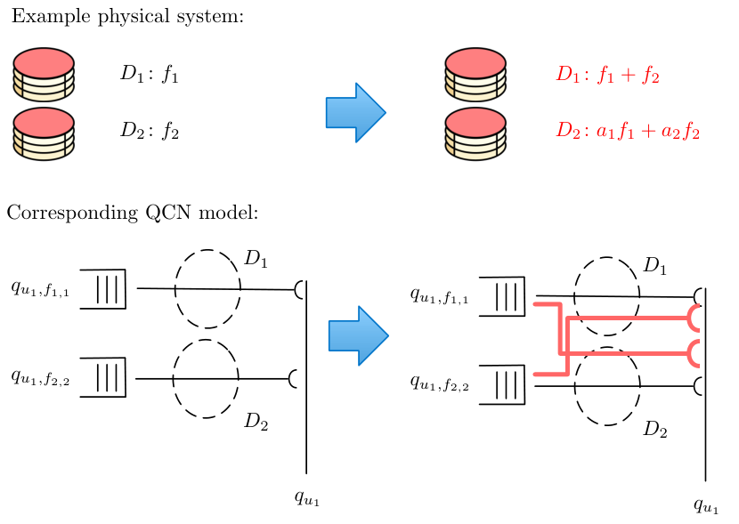
The upper bound for the coded rate region is generated as follows. For each coded chunk stored on (which is a linear combination of chunks in its generation), from each ingress buffer in the set , add a labeled edge or link to sink labeled . See Fig. 8 as a simple single user example, where in the uncoded physical system two unique chunks are stored on unique drives. In the coded physical system, , and , so we add two edges to the coded QCN model, as compared to the uncoded QCN model. In the general case, in constructing this upper bound we assume that any request in an ingress buffer is successfully serviced by sending any coded chunk that has the requested chunk in its generation, and that no penalty is paid for the user needing to wait to decode the chunk of interest by receiving sufficient degrees of freedom.
The upper bound is equivalent to setting all elements of the user’s file knowledge matrix equal to one, in all states. This upper bound can be met if coefficient cycling is performed, where coefficient cycling is the dynamic updating or refreshing of coefficients in a coded chunk such that every degree of freedom request can be served by any coded chunk, as first defined in [24]. Coefficient cycling guarantees reading of chunks from drives without replacement. If chunks are read without replacement within the same generation, then we can then directly apply Algorithm 1. Similar to [25], which considers the achievability of coded storage in systems with an infinite number of storage nodes, we consider achievability given sufficient storage space and chunk layouts on drives. Since it is unclear whether or not coefficient cycling is feasible in all systems, we show that the coded storage upper bound is achievable if all drives store sufficient coded information, even without dynamic coding.44 4 Without loss of generality, we assume each coded chunk is unique and therefore, multisets are not required.
Lemma 5.
Suppose a QCN model operates with a unicast traffic pattern. The coded storage upper bound is achievable if, for every stored on drive , then drive also stores at least additional unique coded chunks from the same generation, .
Proof.
The upper bound holds if all ingress buffers can be served by all valid modes across their connected edges, regardless of any user’s state via . More specifically, select any ingress buffer with connected edges labelled . For any fixed , if in any timeslot, then must hold in all timeslots. If there exists a read request in , then user has received less than innovative degrees of freedom. Due to the unicast traffic pattern, since stores at least unique coded chunks, then no matter which strict subset of chunks stored on has already received, can always serve a coded chunk that is innovative for . Hence, can receive an innovative chunk in every timeslot and if in any timeslot, then in all timeslots. ∎
Lemma 6.
Suppose a QCN model operates with any traffic pattern. The coded storage upper bound is achievable if, for every stored on drive , then drive also stores at least additional unique coded chunks from the same generation .
Proof.
The upper bound holds if all ingress buffers can be served by all their connected edges and valid modes, regardless of . Consider the ingress queues with connected edges labeled . Suppose there exists a subset of users for which user state in some timeslot, and such that in another timeslot. Consider the timeslot in which such that . This implies contains no coded chunk that is innovative for all users . By definition of , all users in are in a state where they have received less than innovative coded chunks. However, the scheduler can then read one of the additional coded chunks, since the drive stores coded chunks from the same generation. We can continue this process for all timeslots until all users have received degrees of freedom, so we have a contradiction. ∎
Note that the uncoded system rate region is a lower bound for the coded storage. See Sec. VII for examples that compare the uncoded RR with the coded RR upper bound.
VII Examples & Numerical Results
This section walks the reader through the generation of an uncoded system’s RR (RR) under a variety of traffic patterns. All examples are of small storage systems to allow for ease of presentation. We then compare the uncoded RR and coded storage RR upper bound.
VII-A Uncoded RR Examples
This subsection walks the reader through simple RR computation examples using our conflict graph and SSP approach.
Ex. 1, one chunk, two users under multicast: Consider a system with two users and and a single chunk stored on drive , under a multicast traffic pattern. Assuming arrival rate of for requests of from user , , and a general multicast scenario, the conflict graph is shown in Fig. 9. In this conflict graph, three stable sets can be found, where the incidence vectors corresponding to these stable sets are as follows
| (18) |
The first, second and third elements of these incidence vectors correspond to vertices , , and , respectively. Based on the above incidence vectors, the and incidence vectors, and , can be expressed as
| (19) |
Since there exists only one drive in the system, the - and -incidence vectors, and , can be obtained as
| (20) |
Using (17), the following system of linear equations can be obtained
| (21) |
The RR corresponding to this system of linear equations is shown in Fig. 9(b), with area of 1.
Ex. 2, one chunk, two users under unicast: Consider Ex. 1 under the unicast traffic pattern, as opposed to multicast. The updated conflict graph is shown in Fig. 10(a). In this conflict graph, two stable sets can be found and the incidence vectors corresponding to these stable sets are as follows
| (22) |
The first and second elements of these incidence vectors correspond to vertices and , respectively. Based on the above incidence vectors and the fact that there exists only one drive in the system, the - and -incidence vectors, and , can be expressed as
| (23) |
By using (17), the following system of linear equations can be obtained
| (24) |
The corresponding rate region is shown in Fig. 10(b), with area of 1/2.
Ex. 3, one chunk, two users under broadcast: Consider Ex. 1 under the broadcast traffic pattern. This example shows that there are caveats in using RR area/volume as a performance metric that should be carefully considered. The conflict graph is shown in Fig. 11(a), in which only one stable set exists, with incidence vector
| (25) |
Based on the above incidence vector, the - and -incidence vectors, and , are
| (26) |
By using (17), the following system of linear equations can be obtained
| (27) |
The corresponding RR is shown in Fig. 11(b), with area of 0.
VII-B Comparison of Uncoded and Coded Storage RR
This subsection compares the RR areas of uncoded storage and the coded storage upper bound. Our coded storage numerical examples use a striped file coded storage layout, which can be seen in [24], and assume . We first walk the reader through a very simple example that demonstrates the increased scheduling flexibility allowed by coded storage. We then summarize other examples across various traffic patterns.
Ex. 4, uncoded, two chunks, one user with : Consider an uncoded system with one user and two chunks and which are stored on drives and , respectively. Assuming arrival rate of for request of from user , , and a multicast with multipacket reception setting, the conflict graph is shown in Fig 12(a). In this conflict graph, three stable sets can be found, where the incidence vectors corresponding to these stable sets are as follows
| (28) |
The first and second elements of these incidence vectors correspond to vertices and , respectively. Based on the above incidence vectors, the - and -incidence vectors, and , can be expressed as
| (29) |
By using (17), the following system of linear equations can be obtained
| (30) |
The RR corresponding to the above system of linear equations is shown in Fig. 12(b), with area 1.
Ex. 5, coded, two chunks, one user with : Now consider Ex. 4 under a coded storage system, where and . The conflict graph of the coded system is shown in Fig 13(a). In this conflict graph, eight stable sets can be found, where the incidence vectors corresponding to these stable sets are as follows
| (31) |
The first, second, third and fourth elements of these incidence vectors correspond to vertices , , and , respectively. Furthermore, based on the above incidence vectors, the , , and -incidence vectors, , , and , can be expressed as
| (32) |
Therefore, the - and -incidence vectors, and , are
| (33) |
Then, by using (17), the following system of linear equations can be obtained
| (34) |
The corresponding rate region can be obtained as shown in Fig. 13(b), of area 2, whereas the uncoded equivalent has area of 1 (as shown in Fig. 12(b)).
Intuition behind this increase is as follows. Suppose two requests are in queue and none are in . In this case, in the uncoded system servicing this would take two timeslots. In comparison, the coded system could service these two requests in one timeslot.
Ex. 6, uncoded and coded, two users, two chunks: Consider an uncoded system with two users , and two chunks and stored on drives and . For the coded system, consider the following drive mapping: and . A comparison of the RR volumes under different traffic patterns and MPR assumptions is presented in Table II. Furthermore, as an example, the conflict graphs for the uncoded and coded systems under a multicast traffic pattern with are illustrated in Fig. 14. Note neither graph is a simple clique. For instance, since multicast is allowed, in the uncoded conflict graph, there are no edges between vertices reading from different drives and transmitting to different users, e.g. between and , and between and . Similarly, for the coded system, there are no edges between vertices of the form and , , where and .
| Traffic Pattern | Uncoded | Coded | % |
| Single unicast | 0.0417 | 0.0417 | 0 |
| Multiple unicast | 0.1667 | 0.25 | 50 |
| Multiple Unicast, with MPR | 0.25 | 0.6667 | 167 |
| Broadcast | 0 | 0 | 0 |
| Broadcast, with MPR | 0 | 0 | 0 |
| Multicast | 0.25 | 0.25 | 0 |
| Multicast, with MPR | 1 | 2.6667 | 167 |
| Average | 54.8 |


Ex. 7, uncoded and coded, two users, three chunks: Consider an uncoded system with two users , and three chunks , , and stored on drives , and . For the coded system, consider the following drive mapping: , and , a comparison of the RR’s volume for this system under different traffic patterns is presented in Table III.
| Traffic Pattern | Uncoded | Coded | % |
| Single unicast | 0.0014 | 0.0014 | 0 |
| Multiple unicast | 0.0236 | 0.0278 | 17.8 |
| Multiple unicast, with MPR | 0.1250 | 1.0125 | 710 |
| Broadcast | 0 | 0 | 0 |
| Broadcast, with MPR | 0 | 0 | 0 |
| Multicast | 0.0278 | 0.0278 | 0 |
| Multicast, with MPR | 1 | 8.1 | 710 |
| Average | 205.4 |
Results show significant increases in RR volume when using coded storage, averaged across traffic patterns, and as traffic patterns change, the bound shows sizable variability in coded storage gains. This encouraging gain is tempered by the fact that it is an upper bound. Yet, the size of such potential increases warrants further and more exact coded storage RR analysis.
VIII Discussion & Conclusions
Potential areas of future work in this area are as follows. Although the QCN model can be used for arbitrary chunk-to-drive mappings, the seeking within drives is assumed to be deterministic. This may be a reasonable model if drives are of particular solid state varieties, but deterministic drive models for HDD are problematic. It would be interesting to extend the model to allow for internal finite buffers at drives themselves, as well as arbitrary service distributions.
The conflict graphs generated by the QCN model are a powerful tool for exploring different traffic patterns. However, the state space of the conflict graphs grows quickly in the general case, and it may be useful to explore special cases of storage and traffic patterns that allow for conflict graphs that may not require particular structures that allow for exact characterization, such as quasi-line conflict graphs.
We have developed an upper bound for coded storage rate regions, which is achievable in certain dynamic coding systems, as well as in certain chunk-to-drive mappings. It would be useful to examine the tightness of this bound, as well as to develop a strict lower bound, or to find an exact solution to the rate region of coded storage. Potential avenues include characterizing coded QCN models via user’s file knowledge matrix directly.
In conclusion, we have developed a method to map a physical storage system into a simple queued cross-bar network model, with particular application to high-traffic storage systems. In doing so, our method and related analysis tools use existing work in arbitrary queueing networks literature, cross-bar switching, as well as conflict graphs. This allows the QCN method as a natural modeling and analysis tool for systems with non-regular chunk-to-drive mappings, replication, as well as for coded storage. We have used a conflict graph approach, which is a function of storage system traffic patterns, to exactly characterize the stable set polytope of the conflict graphs in a number of cases. We have then computed and compared the rate regions of uncoded storage and of the coded storage upper bound, quantifying promising benefits of coded storage over uncoded systems in terms of RR volume. We have also shown how optimal offline and online scheduling algorithms can be generated from our model.
References
- [1] A. G. Dimakis, K. Ramchandran, Y. Wu, and C. Suh, “A survey on network codes for distributed storage,” Proc. IEEE, vol. 99, no. 3, pp. 476–489, Mar. 2011.
- [2] D. Ford, F. Labelle, F. I. Popovici, M. Stokely, V.-A. Truong, L. Barroso, C. Grimes, and S. Quinlan, “Availability in globally distributed storage systems,” in Proceedings of the 9th USENIX conference on Operating systems design and implementation, ser. OSDI’10. Berkeley, CA: USENIX Association, 2010, pp. 1–7. [Online]. Available: http://dl.acm.org/citation.cfm?id=1924943.1924948
- [3] L. Tassiulas and A. Ephremides, “Stability properties of constrained queueing systems and scheduling policies for maximum throughput in multihop radio networks,” IEEE Trans. Autom. Control, vol. 37, no. 12, pp. 1936–1948, Dec. 1992.
- [4] N. B. Shah, K. Lee, and K. Ramchandran, “The MDS Queue: Analysing latency performance of codes and redundant requests,” CoRR, http://arxiv.org/abs/1211.5405, 2012.
- [5] L. Huang, S. Pawar, Z. Hao, and K. Ramchandran, “Codes can reduce queueing delay in data centers,” in Proc. IEEE Int. Symp. on Inf. Theory, Jul. 2012, pp. 2766–2770.
- [6] T. E. Anderson, S. S. Owicki, J. B. Saxe, and C. P. Thacker, “High-speed switch scheduling for local-area networks,” ACM Trans. Comput. Syst., vol. 11, no. 4, pp. 319–352, Nov. 1993. [Online]. Available: http://doi.acm.org/10.1145/161541.161736
- [7] N. McKeown, A. Mekkittikul, V. Anantharam, and J. Walrand, “Achieving 100% throughput in an input-queued switch,” IEEE Trans. Commun., vol. 47, no. 8, pp. 1260–1267, Aug 1999.
- [8] C. Caramanis, M. Rosenblum, M. X. Goemans, and V. Tarokh, “Scheduling algorithms for providing flexible, rate-based, quality of service guarantees for packet-switching in banyan networks,” in In Proc. of the 38th annual conf. on info. sciences and systems (CISS), 2004, pp. 160–166.
- [9] M. A. Marsan, A. Bianco, P. Giaccone, E. Leonardi, and F. Neri, “Multicast traffic in input-queued switches: optimal scheduling and maximum throughput,” IEEE/ACM Trans. Netw., vol. 11, no. 3, pp. 465–477, Jun. 2003. [Online]. Available: http://dx.doi.org/10.1109/TNET.2003.813048
- [10] B. Prabhakar, N. McKeown, and R. Ahuja, “Multicast scheduling for input-queued switches,” vol. 15, no. 5, pp. 855–866, Jun. 1997.
- [11] H. Yu, S. Ruepp, and M. S. Berger, “Multi-level round-robin multicast scheduling with look-ahead mechanism,” in Proc. IEEE Int. Conf. on Commun., Kyoto, Japan, Jun. 2011, pp. 1–5.
- [12] C. Feng and B. Li, Network coding: Fundamentals and applicaions, 1st ed. Academic Press, 2012, ch. Network coding for conten distribution and multimedia streaming in peer-to-peer networks.
- [13] G. N. Rouskas and V. Sivaraman, “Packet scheduling in broadcast WDM networks with arbitrary transceiver tuning latencies,” IEEE/ACM Trans. Netw., vol. 5, no. 3, pp. 359–370, Jun. 1997.
- [14] D. Traskov, M. Heindlmaier, M. Médard, and R. Koetter, “Scheduling for network-coded multicast,” IEEE/ACM Transactions on Networking (TON), vol. 20, no. 5, pp. 1479–1488, 2012.
- [15] M. Kim, J. K. Sundararajan, M. Médard, A. Eryilmaz, and R. Kötter, “Network coding in a multicast switch,” IEEE Trans. Inf. Theory, vol. 57, no. 1, pp. 436–460, 2011.
- [16] D. B. West, Introduction to graph theory, 2nd ed. NJ: Prentice Hall, 2001.
- [17] K. Ross and N. Bambos, “Optimizing capacity in interconnection networks with finite buffers,” in Technical Report UCSC-CRL-07-03, 2007.
- [18] F. Eisenbrand, G. Oriolo, G. Stauffer, and P. Ventura, “The stable set polytope of quasi-line graphs,” Combinatorica, vol. 28, no. 1, pp. 45–67, 2008.
- [19] K. Fouli, J. Casse, I. Sergeev, M. Médard, and M. Maier, “Broadcasting XORs: On the application of network coding in access point-to-multipoint networks,” in MACOM, 2012.
- [20] L. Kleinrock, Queueing theory: Theory. New York: John Wiley & Sons, 1975, vol. 1.
- [21] A. Schrijver, Combinatorial optimization: Polyhedra and efficiency. New York: Springer, 2003.
- [22] M. Grötschel, L. Lovász, and A. Schrijver, Geometric algorithms and combinatorial optimization. Berlin Heidelberg: Springer-Verlag, 1993.
- [23] J. Sundararajan, S. Deb, and M. Médard, “Extending the Birkhoff-von Neumann switching strategy for multicast - on the use of optical splitting in switches,” IEEE J. Sel. Areas Commun., vol. 25, no. 6, pp. 36–50, 2007.
- [24] U. J. Ferner, M. Médard, and E. Soljanin, “Toward sustainable networking: Storage area networks with network coding,” in Proc. Allerton Conf. on Commun., Control and Computing, Champaign, IL, Oct. 2012.
- [25] S. Acedański, S. Deb, M. Médard, and R. Koetter, “How good is random linear coding based distributed network storage?” in Proc. 1st Workshop on Network Coding, Theory, and Applications (Netcod’05), Apr. 2005.