A General Quaternion-valued Gradient Operator and Its Applications to Computational Fluid Dynamics and Adaptive BeamformingThanks: Submitted to the 2014 International Conference on Digital Signal Processing (DSP2014, held in August 2014, Hong Kong) on 29 April 2014 and accepted on 21 May 2014.

We first introduce the definition of differentiation with respect to a quaternion $q$. Assume that $f(q)$ is a function of the quaternion variable $q$, expressed as

$$f(q)=f_{a}+if_{b}+jf_{c}+kf_{d}\;,$$

(1)

where $f(q)$ is in general quaternion-valued. $f(q)$, as well as its components $f_{a}(q)$, $f_{b}(q)$, $f_{c}(q)$, and $f_{d}(q)$, can be viewed as functions of $q_{a}$, $q_{b}$, $q_{c}$ and $q_{d}$, which can be expressed in terms of $q$ and its involutions [9]:

	$\displaystyle q^{i}$	$\displaystyle=$	$\displaystyle-iqi=q_{a}+q_{b}i-q_{c}j-q_{d}k$
	$\displaystyle q^{j}$	$\displaystyle=$	$\displaystyle-jqj=q_{a}-q_{b}i+q_{c}j-q_{d}k$
	$\displaystyle q^{k}$	$\displaystyle=$	$\displaystyle-kqk=q_{a}-q_{b}i-q_{c}j+q_{d}k.$		(2)

As a consequence, we have

	$\displaystyle q_{a}=\frac{1}{4}(q+q^{i}+q^{j}+q^{k})\;,q_{b}=\frac{1}{4i}(q+q^{i}-q^{j}-q^{k})$
	$\displaystyle q_{c}=\frac{1}{4j}(q-q^{i}+q^{j}-q^{k})\;,q_{d}=\frac{1}{4k}(q-q^{i}-q^{j}+q^{k})$

and

	$\displaystyle q+iqi+jqj+kqk$	$\displaystyle=$	$\displaystyle-2q^{*}$
	$\displaystyle q-iqi-jqj-kqk$	$\displaystyle=$	$\displaystyle 4q_{a}.$		(4)

Given the above relations between the involutions and the real and imaginary parts of $q$, $f(q)$ can be regarded as a function of $q$, $q^{i}$, $q^{j}$ and $q^{k}$. Therefore, in what follows, we consider generally a function of $q$ and the involutions, i.e., $f(q,q^{i},q^{j},q^{k})$. Using the Taylor expansion of $f$, the differential $df$ is given by

$$df=\frac{\partial f}{\partial q}dq+\frac{\partial f}{\partial q^{i}}dq^{i}+\frac{\partial f}{\partial q^{j}}dq^{j}+\frac{\partial f}{\partial q^{k}}dq^{k}$$

(5)

Note $\partial f/\partial q$ and $dq$ are both quaternion, therefore they do not commute. On the other hand, $df=df_{a}+idf_{b}+jdf_{c}+kdf_{d}$. Since $df_{a}$ is the differential of a real function of real numbers $q_{a}$, $q_{b}$, $q_{c}$ and $q_{d}$, we have

	$\displaystyle df_{a}(q_{a},q_{b},q_{c},q_{d})$
	$\displaystyle=\frac{\partial f_{a}}{\partial q_{a}}dq_{a}+\frac{\partial f_{a}}{\partial q_{b}}dq_{b}+\frac{\partial f_{a}}{\partial q_{c}}dq_{c}+\frac{\partial f_{a}}{\partial q_{d}}dq_{d}$
	$\displaystyle=\frac{\partial f_{a}}{\partial q_{a}}[\frac{1}{4}(dq+dq^{i}+dq^{j}+dq^{k})]$
	$\displaystyle+\frac{\partial f_{a}}{\partial q_{b}}[\frac{1}{4i}(dq+dq^{i}-dq^{j}-dq^{k})]$
	$\displaystyle+\frac{\partial f_{a}}{\partial q_{c}}[\frac{1}{4j}(dq-dq^{i}+dq^{j}-dq^{k})]$
	$\displaystyle+\frac{\partial f_{a}}{\partial q_{d}}[\frac{1}{4k}(dq-dq^{i}-dq^{j}+dq^{k})]$
	$\displaystyle=\frac{1}{4}(\frac{\partial f_{a}}{\partial q_{a}}-i\frac{\partial f_{a}}{\partial q_{b}}-j\frac{\partial f_{a}}{\partial q_{c}}-k\frac{\partial f_{a}}{\partial q_{d}})dq$
	$\displaystyle+\frac{1}{4}(\frac{\partial f_{a}}{\partial q_{a}}-i\frac{\partial f_{a}}{\partial q_{b}}+j\frac{\partial f_{a}}{\partial q_{c}}+k\frac{\partial f_{a}}{\partial q_{d}})dq^{i}$
	$\displaystyle+\frac{1}{4}(\frac{\partial f_{a}}{\partial q_{a}}+i\frac{\partial f_{a}}{\partial q_{b}}-j\frac{\partial f_{a}}{\partial q_{c}}+k\frac{\partial f_{a}}{\partial q_{d}})dq^{j}$
	$\displaystyle+\frac{1}{4}(\frac{\partial f_{a}}{\partial q_{a}}+i\frac{\partial f_{a}}{\partial q_{b}}+j\frac{\partial f_{a}}{\partial q_{c}}-k\frac{\partial f_{a}}{\partial q_{d}})dq^{k}$		(6)

Similar expressions for $idf_{b}$, $jdf_{c}$, $kdf_{d}$ can be derived in the same way. The sum of the four expressions give an expressions for $df$. Comparing the resulted expression with equation (5), we observe that the coefficient for $dq$ should be the same, hence:

	$\displaystyle\frac{\partial f}{\partial q}$	$\displaystyle=$	$\displaystyle\frac{1}{4}(\frac{\partial f_{a}}{\partial q_{a}}-i\frac{\partial f_{a}}{\partial q_{b}}-j\frac{\partial f_{a}}{\partial q_{c}}-k\frac{\partial f_{a}}{\partial q_{d}})$		(7)
			$\displaystyle+\frac{i}{4}(\frac{\partial f_{b}}{\partial q_{a}}-i\frac{\partial f_{b}}{\partial q_{b}}-j\frac{\partial f_{b}}{\partial q_{c}}-k\frac{\partial f_{b}}{\partial q_{d}})$
			$\displaystyle+\frac{j}{4}(\frac{\partial f_{c}}{\partial q_{a}}-i\frac{\partial f_{c}}{\partial q_{b}}-j\frac{\partial f_{c}}{\partial q_{c}}-k\frac{\partial f_{c}}{\partial q_{d}})$
			$\displaystyle+\frac{k}{4}(\frac{\partial f_{d}}{\partial q_{a}}-i\frac{\partial f_{d}}{\partial q_{b}}-j\frac{\partial f_{d}}{\partial q_{c}}-k\frac{\partial f_{d}}{\partial q_{d}})$
		$\displaystyle=$	$\displaystyle\frac{1}{4}(\frac{\partial f}{\partial q_{a}}-\frac{\partial f}{\partial q_{b}}i-\frac{\partial f}{\partial q_{c}}j-\frac{\partial f}{\partial q_{d}}k)$

Therefore, $\dfrac{\partial f(q)}{\partial q}$ is given by

$$\dfrac{\partial f(q)}{\partial q}=\frac{1}{4}(\displaystyle\frac{\partial{f(q)}}{\partial q_{a}}-\displaystyle\frac{\partial{f(q)}}{\partial q_{b}}i-\displaystyle\frac{\partial{f(q)}}{\partial q_{c}}j-\displaystyle\frac{\partial{f(q)}}{\partial q_{d}}k)$$

(8)

Expressions for $\partial f/\partial q^{i}$, $\partial f/\partial q^{j}$ and $\partial f/\partial q^{k}$ can be derived similarly. Note that, in general $\partial f(q)/\partial q_{b}$ is a quaternion, therefore $\partial f(q)/\partial q_{b}i\neq i\partial f(q)/\partial q_{b}$, i.e., the two factors do not commute. The same argument applies to the last two terms in equation (8).

$f(q)$ can also be viewed as a function of $q^{*}$ and its involutions. Following the same arguments, we can also find the derivative of $f(q)$ with respect to $q^{*}$, which is given by

$$\dfrac{\partial f(q)}{\partial q^{*}}=\frac{1}{4}(\displaystyle\frac{\partial{f(q)}}{\partial q_{a}}+\displaystyle\frac{\partial{f(q)}}{\partial q_{b}}i+\displaystyle\frac{\partial{f(q)}}{\partial q_{c}}j+\displaystyle\frac{\partial{f(q)}}{\partial q_{d}}k)$$

(9)

where $q^{*}=q_{a}-q_{b}i-q_{c}j-q_{d}k$.

With these results, we can then calculate the derivatives of some simple quaternion functions. For example, we easily obtain

$$\frac{\partial q}{\partial q}=1,~\frac{\partial q}{\partial q^{*}}=-\frac{1}{2}\;.$$

(10)

On the other hand, the product rule is not true in general due to the non-commutativity of quaternion products. However, it holds for the differentiation of quaternion-valued functions to real variables. Suppose $f(q)$ and $g(q)$ are two quaternion-valued functions of the quaternion variable $q$, and $q_{a}$ is the real variable. Then we can have the following result

	$\displaystyle\frac{\partial f(q)g(q)}{\partial q_{a}}$	$\displaystyle=$	$\displaystyle\frac{\partial}{\partial q_{a}}(f_{a}+if_{b}+jf_{c}+kf_{d})g$		(11)
		$\displaystyle=$	$\displaystyle\frac{\partial f_{a}g}{\partial q_{a}}+i\frac{\partial f_{b}g}{\partial q_{a}}+j\frac{\partial f_{c}g}{\partial q_{a}}+k\frac{\partial f_{d}g}{\partial q_{a}}$
		$\displaystyle=$	$\displaystyle(f_{a}\frac{\partial g}{\partial q_{a}}+\frac{\partial f_{a}}{\partial q_{a}}g)+i(f_{b}\frac{\partial g}{\partial q_{a}}+\frac{\partial f_{b}}{\partial q_{a}}g)$
			$\displaystyle+j(f_{c}\frac{\partial g}{\partial q_{a}}+\frac{\partial f_{c}}{\partial q_{a}}g)+k(f_{d}\frac{\partial g}{\partial q_{a}}+\frac{\partial f_{d}}{\partial q_{a}}g)$
		$\displaystyle=$	$\displaystyle(f_{a}+if_{b}+jf_{c}+kf_{d})\frac{\partial g}{\partial q_{a}}$
			$\displaystyle+(\frac{\partial f_{a}}{\partial q_{a}}+i\frac{\partial f_{b}}{\partial q_{a}}+j\frac{\partial f_{c}}{\partial q_{a}}+k\frac{\partial f_{d}}{\partial q_{a}})g$
		$\displaystyle=$	$\displaystyle f(q)\frac{\partial g(q)}{\partial q_{a}}+\frac{\partial f(q)}{\partial q_{a}}g(q)$

When the quaternion variable $q$ is replaced by a quaternion-valued vector w, given by

$$\textbf{w}=[w_{1}~w_{2}~\cdots~w_{M}]^{T}$$

(12)

where $w_{m}=a_{m}+b_{m}i+c_{m}j+d_{m}k$, $m=1,...,M$, the differentiation of $f(\textbf{w})$ with respect to w can be derived using a combination of (8) as follows

$\displaystyle\dfrac{\partial f}{\partial\textbf{w}}=\frac{1}{4}\left[\begin{matrix}\frac{\partial f}{\partial a_{1}}-\frac{\partial f}{\partial b_{1}}i-\frac{\partial f}{\partial c_{1}}j-\frac{\partial f}{\partial d_{1}}k\\ \frac{\partial f}{\partial a_{2}}-i\frac{\partial f}{\partial b_{2}}i-\frac{\partial f}{\partial c_{2}}j-\frac{\partial f}{\partial d_{2}}k\\ \vdots\\ \frac{\partial f}{\partial a_{M}}-\frac{\partial f}{\partial b_{M}}i-\frac{\partial f}{\partial c_{M}}j-\frac{\partial f}{\partial d_{M}}k\end{matrix}\right]$

(13)

Similarly, we define $\dfrac{\partial f}{\partial\textbf{w}^{*}}$ as

$\displaystyle\dfrac{\partial f}{\partial\textbf{w}^{*}}=\frac{1}{4}\left[\begin{matrix}\frac{\partial f}{\partial a_{1}}+\frac{\partial f}{\partial b_{1}}i+\frac{\partial f}{\partial c_{1}}j+\frac{\partial f}{\partial d_{1}}k\\ \frac{\partial f}{\partial a_{2}}+\frac{\partial f}{\partial b_{2}}i+\frac{\partial f}{\partial c_{2}}j+\frac{\partial f}{\partial d_{2}}k\\ \vdots\\ \frac{\partial f}{\partial a_{M}}+\frac{\partial f}{\partial b_{M}}i+\frac{\partial f}{\partial c_{M}}j+\frac{\partial f}{\partial d_{M}}k\end{matrix}\right]$

(14)

Obviously, when $M=1$, (13) and (14) are reduced to (8) and (9), respectively.

The output $y[n]$ and error $e[n]$ of a standard adaptive filter can be expressed as

	$\displaystyle y[n]$	$\displaystyle=$	$\displaystyle{\textbf{w}^{T}[n]}{\textbf{x}[n]}$		(15)
	$\displaystyle e[n]$	$\displaystyle=$	$\displaystyle d[n]-{\textbf{w}^{T}[n]}{\textbf{x}[n]},$		(16)

where $\textbf{w}[n]$ is the adaptive weight vector with a length of $M$, $d[n]$ is the reference signal, $\textbf{x}[n]=[x[n-1],x[n-2],\cdots,x[n-M]]^{T}$ is the input sample sequence, and $\{\cdot\}^{T}$ denotes the transpose operation. The cost function with the quaternion-valued error is $J_{0}[n]=e[n]e^{*}[n]$. Its gradient is given by

	$\displaystyle\nabla_{\textbf{w}^{*}}J_{0}[n]=\frac{\partial{J_{0}[n]}}{\partial\textbf{w}^{*}}$		(17)
	$\displaystyle\nabla_{\textbf{w}}J_{0}[n]=\frac{\partial{J_{0}[n]}}{\partial\textbf{w}}$		(18)

with respect to $\textbf{w}^{*}[n]$ and $\textbf{w}[n]$, respectively. According to [10, 11], the conjugate gradient gives the maximum steepness direction for the optimization surface. Therefore, the conjugate gradient $\nabla_{\textbf{w}^{*}}J_{0}[n]$ will be used to derive the update of the coefficient weight vector.

First we have

	$\displaystyle J_{0}[n]=d[n]d^{*}[n]-d[n]{\textbf{x}^{H}[n]}{\textbf{w}^{*}[n]}-{\textbf{w}^{T}[n]}{\textbf{x}[n]}d^{*}[n]$
	$\displaystyle+{\textbf{w}^{T}[n]}{\textbf{x}[n]}{\textbf{x}^{H}[n]}{\textbf{w}^{*}[n]}$		(19)

For different parts, we obtain the following results

$$\frac{\partial(d[n]d^{*}[n])}{\partial{\textbf{w}^{*}[n]}}=0$$

(20)

$$\frac{\partial(d[n]{\textbf{x}^{H}[n]}{\textbf{w}^{*}[n]})}{\partial{\textbf{w}^{*}[n]}}=d[n]\textbf{x}^{*}[n]$$

(21)

$$\frac{\partial({\textbf{w}^{T}[n]}{\textbf{x}[n]}d^{*}[n])}{\partial{\textbf{w}^{*}[n]}}=-\frac{1}{2}d[n]\textbf{x}^{*}[n]$$

(22)

$$\frac{\partial({\textbf{w}^{T}[n]}{\textbf{x}[n]}{\textbf{x}^{H}[n]}{\textbf{w}^{*}[n]})}{\partial{\textbf{w}^{*}[n]}}=\frac{1}{2}{\textbf{w}^{T}[n]}{\textbf{x}[n]}{\textbf{x}^{*}[n]}$$

(23)

Then we have the final gradient result

$$\nabla_{\textbf{w}^{*}}J_{0}[n]=-\frac{1}{2}e[n]\textbf{x}^{*}[n].$$

(24)

With the general update equation for the weight vector

$$\textbf{w}[n+1]=\textbf{w}[n]-\mu\nabla_{\textbf{w}^{*}}J_{0}[n],$$

(25)

we arrive at the following update equation for the QLMS algorithm with step size $\mu$

$$\textbf{w}[n+1]=\textbf{w}[n]+\mu(e[n]\textbf{x}^{*}[n]).$$

(26)

Recently, to fully exploit the second-order statistics of the signals, an augmented formulation of the data vector has been proposed, first for complex-valued signals and then for quaternion-valued ones. For complex-valued signals, the augmented vector is composed of the original data and its conjugate, while for the latter, due to existence of the three perpendicular quaternion involutions, the choice for the augmented vector is not unique. Without loss of generality, here we adopt the simplest formulation by combining the data vector $\textbf{x}[n]$ and its conjugate $\textbf{x}^{*}[n]$ to produce an augmented vector $\textbf{x}_{a}[n]=\big[\textbf{x}^{T}[n]~~\textbf{x}^{H}[n]\big]^{T}$ [12], where $\{\cdot\}^{H}$ is a combination of the operations of $\{\cdot\}^{T}$ and $\{\cdot\}^{*}$ for a quaternion. For such a “widely linear” model, the quaternion-valued output for the conjugate part of the input is given by

$$\hat{y}[n]=\textbf{g}^{T}[n]\textbf{x}^{*}[n],$$

(27)

where $\textbf{g}[n]$ denotes the weight vector for the conjugate part of the input $\textbf{x}[n]$.

As to the AQLMS algorithm, the update of the weight vector of the conjugate part $\textbf{g}[n]$ can be found with the same method as that of the QLMS in (26), i.e.

$$\textbf{g}[n+1]=\textbf{g}[n]+\mu(e[n]\textbf{x}[n]).$$

(28)

With the augmented weight vector $\textbf{h}_{a}[n]$ defined as

$$\textbf{h}_{a}[n]=\big[\textbf{w}^{T}[n]~~\textbf{g}^{T}[n]\big]^{T},$$

(29)

we obtain the following update equation

$$\textbf{h}_{a}[n+1]=\textbf{h}_{a}[n]+\mu(e_{a}[n]{\textbf{x}_{a}}^{*}[n])$$

(30)

where $e_{a}[n]=d[n]-{\textbf{h}_{a}}^{T}[n]\textbf{x}_{a}[n]$.

The Navier-Stokes equations are the basis of fluid problems. They are essentially the mathematical formulation of the Newton’s second law applied to fluid motions. The general expression of the equations is

$$\rho(\frac{\partial\textbf{u}}{\partial t}+(\textbf{u}\cdot\nabla)\textbf{u})=-\nabla{P}+\eta\Delta{\textbf{u}}$$

(31)

where u is the fluid velocity at a particular spatial location at a given time, $P$ is the pressure and $\rho$ is the fluid density. The left hand side of the equation is the acceleration of the fluid, whilst on the right side are (the gradient of) the forces, including pressure and viscous force. Together with the conservation of mass and suitable boundary conditions, the Navier-Stokes equations can model a large class of fluid motions accurately [13].

The second term on the left hand side of equation (31) represents the contribution from the advection of fluid particles to fluid acceleration, and is customarily called the inertial force. The second term on the right hand side represents the viscous force. The ratio of these two forces is defined as the Reynolds number ($Re$). As it turns out, when $Re$ is large, the flows tend to become unstable and generate a spectrum of high frequency components in the velocity signal. Such a regime of fluid motions is called turbulence. Atmospheric flows, including the wind fields around wind farms, are always turbulence [14]. Due to the presence of the high frequency components, the CFD calculation of the velocity signal in turbulent wind fields becomes very time consuming unless simplifying models are introduced.

DNS solves the Navier-Stokes equations directly without any turbulence models. The advantage of this method is that it is simple as well as accurate with complete information. However, the computational cost can be very high if $Re$ is large. Therefore, this method is not yet applicable to practical situations, for example, the atmospheric flows we will deal with [13]. Nevertheless, as a first step, we choose to use DNS to generate the velocity signals in this study.

The velocity signals are generated by DNS, where the Navier-Stokes equations are solved using a pseudo-spectral method. The CFD code is written in FORTRAN 90. Running the code, we generate a time series of three dimensional turbulent wind velocity fields in a 3-D periodic box. We consider the flow field as an idealized wind field with the mean velocity having been subtracted, and the signal normalized.

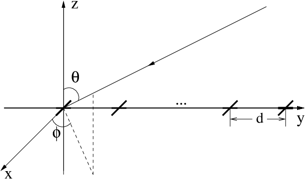
A uniform linear array (ULA) with $M$ crossed-dipole pairs is shown in Fig. 1. These pairs are located along the y-axis with an adjacent spacing $d$, and at each location the two crossed components are parallel to x-axis and y-axis, respectively. Assume there is a far-field incident signal with direction of arrival (DOA) defined by the angles $\theta$ and $\phi$ impinging upon the array from the y-z plane, so that $\phi=\pi/2$ as well as $\phi=-\pi/2$, and $0\leq\theta\leq\pi/2$. As a result, the spatial steering vector for the signal is expressed as

	$\displaystyle\textbf{S}_{c}(\theta,\phi)$	$\displaystyle=$	$\displaystyle[1,e^{-j2\pi dsin{\theta}sin{\phi}/{\lambda}},$		(32)
			$\displaystyle\cdots,e^{-j2\pi(M-1)dsin{\theta}sin{\phi}/{\lambda}}]^{T}$

where $\lambda$ is the wavelength of the incident signal. For a crossed dipole the spatial-polarization coherent vector can be given by [15, 16]

$$\textbf{S}_{p}(\theta,\phi,\gamma,\eta)=\begin{cases}[-cos{\gamma},cos{\theta}sin{\gamma}e^{j\eta}]&\text{for $\phi=\pi/2$}\\ [cos{\gamma},-cos{\theta}sin{\gamma}e^{j\eta}]&\text{for $\phi=-\pi/2$}\end{cases}$$

(33)

where $\gamma$ is the auxiliary polarization angle with $\gamma\in[0,\pi/2]$, and the $\eta\in[-\pi,\pi]$ is the polarization phase difference.

The array structure can be divided into two sub-arrays. One is parallel to the x-axis and the other is parallel to the y-axis. The complex-valued steering vector of the x-axis sub-array is given by

$$\textbf{S}_{x}(\theta,\phi,\gamma,\eta)=\begin{cases}-cos{\gamma}\textbf{S}_{c}(\theta,\phi)&\text{for $\phi=\pi/2$}\\ cos{\gamma}\textbf{S}_{c}(\theta,\phi)&\text{for $\phi=-\pi/2$}\end{cases}$$

(34)

and for the y-axis it is expressed as

$$\textbf{S}_{y}(\theta,\phi,\gamma,\eta)=\begin{cases}cos{\theta}sin{\gamma}e^{j\eta}\textbf{S}_{c}(\theta,\phi)&\text{for $\phi=\pi/2$}\\ -cos{\theta}sin{\gamma}e^{j\eta}\textbf{S}_{c}(\theta,\phi)&\text{for $\phi=-\pi/2$}\end{cases}$$

(35)

Combining these two steering vectors together, we have a quaternion-valued composite steering vector given as below

$$\textbf{S}_{q}(\theta,\phi,\gamma,\eta)=\textbf{S}_{x}(\theta,\phi,\gamma,\eta)+i\textbf{S}_{y}(\theta,\phi,\gamma,\eta).$$

(36)

The response of the array is

$\displaystyle r(\theta,\phi,\gamma,\eta)=\textbf{w}^{H}\textbf{S}_{q}(\theta,\phi,\gamma,\eta)$

(37)

where w is the quaternion-valued weight vector.

When a reference signal $d[n]$ is available, adaptive beamforming can be implemented by the standard adaptive filter structure, as shown in Fig. 2, where $x_{m}[n]$, $m=1,2,\cdots,M$ are the received quaternion-valued vector sensor signals, $w_{m}[n]$, $m=1,2,\cdots,M$ are the corresponding quaternion-valued coefficients, $y[n]$ is the beamformer output and $e[n]$ is the error signal.

In this part, both the QLMS and the AQLMS algorithms are applied to the wind data generated by CFD simulations with a sampling frequency of 1 Hz. The parameters are as follows. The step size is $\mu=2.5\times 10^{-4}$ and the adaptive filter length is $L=16$. The prediction step is 2. The adaptive weight vector is initialized as an all-zero vector. Fig. 3 and Fig. 4 show the results for the QLMS and AQLMS algorithms, respectively. As we can see from the results, both algorithms can track the change of the wind speed signal effectively.

Now we run simulations for the adaptive beamforming scenario. The vector sensor array with 10 crossed-dipoles and half-wavelength spacing is considered to obtain the output using the QLMS algorithm. The stepsize $\mu$ here is set to be $1\times 10^{-6}$. A desired signal with 20 dB SNR impinges from the broadside and two interfering signals with the signal to interference ratio (SIR) of 0 dB arrive from $30^{\circ}$ and $-20^{\circ}$, respectively. All the signals have the same polarisation of $(\gamma,\eta)=(0,0)$. The learning curve averaged over 100 simulation runs is shown in Fig. 5, where we can see the normalised error has reached about -10 dB, indicating an effective beamforming operation.

References

- [1] N. Le Bihan and J. Mars, “Singular value decomposition of quaternion matrices: a new tool for vector-sensor signal processing,” Signal Processing, vol. 84, no. 7, pp. 1177–1199, 2004.
- [2] X. R. Zhang, W. Liu, Y. G. Xu, and Z. W. Liu, “Quaternion-valued robust adaptive beamformer for electromagnetic vector-sensor arrays with worst-case constraint,” Signal Processing, vol. 104, pp. 274–283, November 2014.
- [3] M. B. Hawes and W. Liu, “A quaternion-valued reweighted minimisation approach to sparse vector sensor array design,” in Proc. of the International Conference on Digital Signal Processing, Hong Kong, August 2014.
- [4] C. C. Took and D. P. Mandic, “The quaternion LMS algorithm for adaptive filtering of hypercomplex processes,” IEEE Transactions on Signal Processing, vol. 57, no. 4, pp. 1316–1327, 2009.
- [5] M. D. Jiang, W. Liu, Y. Li, and X. R. Zhang, “Frequency-domain quaternion-valued adaptive filtering and its application to wind profile prediction,” in Proc. of the IEEE TENCON Conference, Xi’an, China, October 2013.
- [6] H. L. Van Trees, Optimum Array Processing, Part IV of Detection, Estimation, and Modulation Theory. New York: Wiley, 2002.
- [7] W. Liu and S. Weiss, Wideband Beamforming: Concepts and Techniques. Chichester, UK: John Wiley & Sons, 2010.
- [8] A. Nehorai, K. C. Ho, and B. T. G. Tan, “Minimum-noise-variance beamformer with an electromagnetic vector sensor,” IEEE Transactions on Signal Processing, vol. 47, no. 3, pp. 601–618, March 1999.
- [9] T. A. Ell and S. J. Sangwine, “Quaternion involutions and anti-involutions,” Computers & Mathematics with Applications, vol. 53, no. 1, pp. 137–143, 2007.
- [10] D. P. Mandic, C. Jahanchahi, and C. C. Took, “A quaternion gradient operator and its applications,” IEEE Signal Processing Letters, vol. 18, no. 1, pp. 47–50, 2011.
- [11] D. Brandwood, “A complex gradient operator and its application in adaptive array theory,” in IEE Proceedings H (Microwaves, Optics and Antennas), vol. 130, no. 1. IET, 1983, pp. 11–16.
- [12] C. C. Took and D. P. Mandic, “A quaternion widely linear adaptive filter,” IEEE Transactions on Signal Processing, vol. 58, no. 8, pp. 4427–4431, 2010.
- [13] J. Ferzige and M. Peric, Computational methods for fluid dynamics. Springer, 2001.
- [14] S. B. Pope, Turbulent flows. Cambridge university press, 2000.
- [15] R. Compton Jr, “On the performance of a polarization sensitive adaptive array,” IEEE Transactions on Antennas and Propagation, vol. 29, no. 5, pp. 718–725, 1981.
- [16] J. Li and R. Compton Jr, “Angle and polarization estimation using esprit with a polarization sensitive array,” IEEE Transactions on Antennas and Propagation, vol. 39, pp. 1376–1383, 1991.