Exact simulation of Brown-Resnick random fields at a finite number of locations

Max-stable random fields are fundamental models for spatial extremes. These models have been coined by de Haan [9], and have recently found applications to extreme meteorological events such as rainfall modeling and extreme temperatures (Buishand et al. [3], de Haan and Zhou [10], Dombry et al. [6], Davis et al. [4], Huser and Davison [11]). There are three different kinds of normalized max-stable processes, with Gumbel, Fréchet, and Weibull marginals, respectively. In what follows, we restrict ourselves to max-stable processes with Gumbel marginals; corresponding results for Fréchet and Weibull marginals can be obtained by a monotone transformation of the Gumbel case.

This paper studies a particular class of max-stable random fields known as Brown-Resnick random fields. Simulation of these and related processes is complicated, and the literature exclusively focuses on approximate simulation techniques; see for example Schlather [21], Oesting et al. [16], Engelke et al. [8], Oesting and Schlather [17], Dombry et al. [6].

This paper is the first to devise an exact simulation method for Brown-Resnick random fields. The key ingredient is a new representation for Brown-Resnick random fields, which is of independent interest. In fact, we show that there is an uncountable family of representations. At the heart of our derivation of these representations lies a change of measure argument.

The representation (1.1) is not particularly suitable for exact sampling. Although $(V_{i})$ and $(W_{i})$ are easily simulated, it turns out that the naive simulation approach of replacing $\sup_{i\geq 1}$ by $\sup_{i\leq N}$ for some large $N$, may fail. For example, assume that $W_{i}$ is standard Brownian motion on ${\mathbb{R}}$. Then, in view of the law of the iterated logarithm, each of the processes $W_{i}(t)-\sigma^{2}(t)/2$ drifts to $-\infty$ a.s. as $t\to\infty$. In turn, the process $\sup_{i\leq N}\big(V_{i}+W_{i}(t)-\sigma^{2}(t)/2\big)$ drifts to $-\infty$ as $t\to\infty$ as well. In particular, the simulation of $\eta$ requires an increasing number $N$ if one aims at a sample path of the process on a larger interval. More importantly, it is unclear how $N$ should be chosen.

Using our new representations, we obtain an exact sampling method for $\eta$ at the points $t_{1},\ldots,t_{n}\in{\mathbb{R}}^{d}$, meaning that the output of the method has the same distribution as $(\eta(t_{1}),\ldots,\eta(t_{n}))$. In our method, it is no longer problematic that the processes $W_{i}(t)-\sigma^{2}(t)/2$ drift away to $-\infty$ and a truncation point is automatically identified by our algorithm.

Several properties of Brown-Resnick processes readily follow from our representations, although they are not straightforward to see from (1.1). For instance, the process $\eta$ is stationary in the sense that $\eta$ has the same distribution as $\eta(\cdot+c)$ for any choice of $c\in{\mathbb{R}}^{d}$. The process $\eta$ also has standard Gumbel marginals. In deriving our representations from (1.1), $\sigma^{2}$ drops out and we recover the known fact that the law of $\eta$ only depends on the variogram

These properties were proved in Kabluchko et al. [13] with arguably more elaborate techniques.

Given an exact simulation method for the Brown-Resnick process with Gumbel marginals, we also have an exact simulation method for this process with Fréchet or Weibull marginals. For example, the processes ${\rm e}\,^{\eta}$ and $-{\rm e}\,^{-\eta}$ have Fréchet $\Phi_{1}(x)={\rm e}\,^{-x^{-1}}$, $x>0$, and Weibull $\Psi_{1}(x)={\rm e}\,^{-|x|}$, $x<0$, marginals, respectively.

In this section we provide new representations for the Brown-Resnick random field $\eta$ given in (1.1). These representations arise from a change of measure. We make the same assumptions on the stationary Brown-Resnick process as in the previous section. All proofs for this section are in Section 5. We fix the functions $\sigma^{2}$ and $\gamma$ throughout this section.

The following theorem is the main result of this section.

Theorem 2.1 leads to the following three well known facts proved in Kabluchko et al. [13].

This section presents a simulation algorithm for Brown-Resnick random fields on a discrete set of points $t_{1},\ldots,t_{n}\in\mathbb{R}^{d}$. We may assume that $\sigma^{2}/2=\gamma$ in this section. Since Theorem 2.1 gives a different representation for each choice of $\mu$, it would be interesting to know which choice leads to the fastest algorithm. Here we simply let $\mu$ be uniform on $\{t_{1},\ldots,t_{n}\}$.

Remark 2.4 shows that the vector $(N(t_{1}),\ldots,N(t_{n}))$ with, for $j=1,\ldots,n$,

has the same distribution as $(\eta(t_{1}),\ldots,\eta(t_{n}))$, where $\big((V_{i},T_{i})\big)_{i\geq 1}$ belong to a Poisson process on ${\mathbb{R}}\times\{t_{1},\ldots,t_{n}\}$ with intensity measure ${\rm e}\,^{-x}dx\times\big(n^{-1}\sum_{i=1}^{n}\delta_{t_{i}}(dy)\big)$. We slightly rewrite the above display as

This is the representation we use for our simulation algorithm.

A point $V_{i}$ on $\mathbb{R}$ gives rise to a ‘cluster’ of points $\{C_{i}(t_{j}):j=1,\ldots,n\}$ with

These cluster points can be visualized by interpreting them as belonging to different levels depending on the value of $j$; see Figure 1. The variable $N(t_{j})=\sup_{i\geq 1}C_{i}(t_{j})$ is then the maximum of all cluster points on the $j$-th level. The crucial insight is that only a finite number of points/cluster pairs $(V_{i},C_{i})$ need to be generated, since $C_{i}(t_{j})\leq V_{i}+\log n$ and we seek $\sup_{i\geq 1}C_{i}(t_{j})$ for $j=1,\ldots,n$. The algorithm generates points/cluster pairs $(V+\log n,C)$ in decreasing order of $(V+\log n)$-value, until the next $(V+\log n)$-value is smaller than the current maximum over the cluster points on each level. For instance, in Figure 1, after $V_{3}+\log 4$ has been generated, none of the remaining cluster points can change the values of $(N(t_{1}),\ldots,N(t_{4}))$, which have been given a different color.

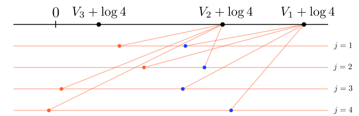
To get a sense of how many points of $V$ will be generated, let us consider the (degenerate) case where $t_{1}=\cdots=t_{n}=t$. We then have $C_{i}(t_{j})=V_{i}$ for $j=1,\ldots,n$, so the algorithm terminates after generating $\inf\{M:V_{M}+\log n<V_{1}\}$ points of $V$. For large $n$, this implies that the number of points is of order $n$.

We remark that this algorithm is suitable for parallelization. Indeed, several points of the $V$-process can be generated simultaneously instead of one at the time, with corresponding clusters being computed on different processors. Specifically, with one master and $K$ workers, the algorithm would consist of a number of steps, each of which computes the next $K$ clusters in parallel. At each step of the algorithm, the master generates the next $K$ $V$-points in decreasing order. This is readily done since the points $({\rm e}\,^{-V_{i}})$ constitute a standard Poisson process on $\mathbb{R}_{+}$. Each of the $K$ clusters would then be computed on a worker node, after which the master checks whether the algorithm can be terminated or whether further steps are needed.

This section reports on several simulation experiments we have carried out in order to validate our algorithm and to test its performance in terms of speed. Throughout, we work with Brown-Resnick random fields with variogram $\gamma(t)=|t|^{\alpha}/2$ for some $\alpha\in(0,2]$. Appendix A has some implementation details.

This section presents the proof of Theorem 2.1 We fix the functions $\sigma^{2}$ and $\gamma$ throughout this section. Contrary to the preceding two sections, we do not assume that $\gamma=\sigma^{2}/2$ but we shall see that the function $\sigma^{2}$ vanishes from our calculations.

We start with an auxiliary lemma; see de Haan [9] and Kabluchko et al. [13] for proofs.

The following change of measure lemma plays a key role in our argument, and shows why the variance function $\sigma^{2}$ vanishes from the calculations. It is a field version of Lemma 1 in Dieker and Yakir [5], see also [12, Prop. 2] for the underlying change of measure result. We only sketch the key idea of the proof insofar as it highlights the differences with [5], since the lemma follows from the same arguments as given there.

The authors are grateful to the organizers of the workshop Stochastic Networks And Risk Analysis IV in Bedlewo, Poland, where much of this work was completed. TM thanks Liang Peng for inviting him to Georgia Tech in April 2013, when this work was initiated. ABD is supported in part by NSF CAREER grant CMMI-1252878, and TM by DFF grant 4002-00435. We thank the anonymous referees for their constructive comments and suggestions.

References

- [2] Brown, B. and Resnick, S.I. (1977) Extreme values of independent stochastic processes. J. Appl. Probab. 14, 732–739.
- [3] Buishand, T., Haan, L. de and Zhou, C. (2008) On spatial extremes: with applications to a rainfall problem. Ann. Appl. Stat. 2, 624–642.
- [4] Davis, R.A., Klüppelberg, C. and Steinkohl, C. (2013) Statistical inference for max-stable processes in space and time. J. Royal Statist. Soc. Series B. 75, 791–819.
- [5] Dieker, A. B. and Yakir, B. (2014) On asymptotic constants in the theory of Gaussian processes. Bernoulli 20, 1600–1619.
- [6] Dombry, C., Éyi-Minko, F. and Ribatet, M. (2013) Conditional simulation of max-stable processes. Biometrika 100, 111–124.
- [7] Embrechts, P., Klüppelberg, C. and Mikosch, T. (1997) Modelling Extremal Events for Insurance and Finance. Springer, Berlin.
- [8] Engelke, S., Kabluchko, Z and Schlather, M. (2011) An equivalent representation of the Brown-Resnick process. Stat. Probab. Letters 81, 1150–1154.
- [9] Haan, L. de (1984) A spectral representation for max-stable processes. Ann. Probab. 12, 1194–1204.
- [10] Haan, L. de and Zhou, C. (2008) On extreme value analysis of a spatial process. REVSTAT 6, 71–81.
- [11] Huser, R. and Davison, A.C. (2014) Space-time modelling for extremes. J. Royal Statist. Soc. Series B. 76, 439–461.
- [12] Kabluchko, Z. (2009) Spectral representations of sum- and max-stable processes. Extremes 12, 401–424.
- [13] Kabluchko, Z., Schlather, M. and Haan, L de (2009) Stationary max-stable fields associated to negative definite functions. Ann. Probab. 37, 2042–2065.
- [14] Kroese, D.P. and Botev, Z.I. (2013) Spatial process generation. In: Schmidt, V. (Ed.). Lectures on Stochastic Geometry, Spatial Statistics and Random Fields. Volume II: Analysis, Modeling and Simulation of Complex Structures. Springer-Verlag, Berlin.
- [15] Leadbetter, M.R., Lindgren, G. and Rootzén, H. (1983) Extremes and Related Properties of Random Sequences and Processes. Springer, Berlin.
- [16] Oesting, M., Kabluchko, Z. and Schlather, M. (2012) Simulation of Brown-Resnick processes. Extremes 15, 89–107.
- [17] Oesting, M. and Schlather, M. (2014) Conditional sampling for max-stable processes with a mixed moving maxima representation. Extremes, 17, 157–192.
- [18] Oesting, M., Schlather M. and Zhou, C. (2013) On the normalized spectral representation of max-stable processes on a compact set. Preprint available from http://arxiv.org/abs/1310.1813.
- [19] Piterbarg, V.I. (1996) Asymptotic Methods in the Theory of Gaussian Processes and Fields. AMS Translations and Mathematical Monographs. 148.
- [20] The R Project for Statistical Computing; see http://www.r-project.org/.
- [21] Schlather, M. (2002) Models for stationary max-stable random fields. Extremes 5, 33–44.
- [22] Nguyen Xuan Xanh (1979) Ergodic theorems for subadditive spatial processes. Z. Wahrscheinlichkeitstheorie verw. Gebiete 48, 159–176.