Consistently Orienting Facets in Polygon Meshes by
Minimizing the Dirichlet Energy of Generalized Winding Numbers

As a preprocessing step, facets that are topologically connected and forming a two-manifold surface are grouped together as a patch, similar to Borodin et al.’s method [BZK04]. If the mesh has non-manifold edges, the mesh is split around these edges, and multiple patches are generated. All facets belonging to the same patch share the same decision about whether they should be flipped or not in the output. Given $n$ patches, our goal is to seek an assignment for $n$ binary variables representing whether the $i$-th patch $\mathcal{P}_{i}$ should be flipped or not ($1\leq i\leq n$).

Let us first review the concept of generalized winding numbers [JKSH13]. The generalized winding number (hereafter we drop the word “generalized”) at a point $\mathbf{p}\in\mathds{R}^{3}$ is defined as

$$w(\mathbf{p})=\frac{1}{4\pi}\sum_{\tau\in\mathcal{M}}\theta_{\tau}(\mathbf{p})\ ,$$

(1)

where $\mathcal{M}$ is the input mesh (denoted as a set of facets), $\tau\in\mathcal{M}$ is a facet in $\mathcal{M}$, and $\theta_{\tau}$ is the signed solid angle subtended by $\tau$ viewed from $\mathbf{p}$. Note that the sign of the angle is defined to be positive for points in the half space corresponding to the back side of a facet. In particular, the winding number of points inside and outside a watertight mesh is 1 and 0, respectively.

Since the winding number of a watertight and consistently oriented mesh is piecewise constant and hence its Dirichlet energy is zero, our intuition is that the Dirichlet energy of the winding number for an imperfect mesh should decrease as its facet orientations become more consistent. We give a mathematical formulation of the Dirichlet energy in the following.

For each $i$-th patch $\mathcal{P}_{i}\subseteq\mathcal{M}\ (1\leq i\leq n)$, we want to determine a binary variable $s_{i}\in\{+1,-1\}$ called sign, where $s_{i}=-1$ means that all facets in $\mathcal{P}_{i}$ should be flipped in the output. Now we can define the winding number with respect to the given sign $\mathbf{s}=(s_{1},\cdots,s_{n})$ as

$$w_{\mathbf{s}}(\mathbf{p})=\frac{1}{4\pi}\sum_{i=1}^{n}s_{i}\sum_{\tau\in\mathcal{P}_{i}}\theta_{\tau}(\mathbf{p})\ .$$

(2)

Note that the orientation of each triangle $\tau$ is fixed to the original configuration when computing $\theta_{\tau}$. The Dirichlet energy of $w_{\mathbf{s}}$ denoted as $E(\mathbf{s})$ is a function of $\mathbf{s}$ and is defined as the integral of the gradient magnitude squared of $w_{\mathbf{s}}$ over the volumetric domain $\Omega=\mathds{R}^{3}\setminus\mathcal{M}$:

$$E(\mathbf{s})=\int_{\mathbf{p}\in\Omega}\left\|\nabla w_{\mathbf{s}}(\mathbf{p})\right\|^{2}dV\ .$$

(3)

Reorganizing the integrand as

	$\displaystyle\left\|\nabla w_{\mathbf{s}}(\mathbf{p})\right\|^{2}$	$\displaystyle=$	$\displaystyle\left\|\frac{1}{4\pi}\sum_{i=1}^{n}s_{i}\sum_{\tau\in\mathcal{P}_{i}}\nabla\theta_{\tau}(\mathbf{p})\right\|^{2}$		(4)
		$\displaystyle=$	$\displaystyle\frac{1}{16\pi^{2}}\left(\sum_{i=1}^{n}s_{i}\sum_{\tau\in\mathcal{P}_{i}}\nabla\theta_{\tau}(\mathbf{p})\right)\cdot\left(\sum_{j=1}^{n}s_{j}\sum_{\mu\in\mathcal{P}_{j}}\nabla\theta_{\mu}(\mathbf{p})\right)$		(5)
		$\displaystyle=$	$\displaystyle\frac{1}{16\pi^{2}}\sum_{i=1}^{n}\sum_{j=1}^{n}s_{i}s_{j}\left(\sum_{\tau\in\mathcal{P}_{i}}\nabla\theta_{\tau}(\mathbf{p})\right)\cdot\left(\sum_{\mu\in\mathcal{P}_{j}}\nabla\theta_{\mu}(\mathbf{p})\right),$		(6)

the energy can be written concisely in quadratic form as

$$E(\mathbf{s})=\mathbf{s}^{\top}\mathbf{Q}\ \mathbf{s}\ ,$$

(7)

where $Q$ is an $n$-by-$n$ matrix with elements

$$Q_{ij}=\frac{1}{16\pi^{2}}\sum_{\tau\in\mathcal{P}_{i}}\sum_{\mu\in\mathcal{P}_{j}}\int_{\mathbf{p}\in\Omega}\nabla\theta_{\tau}(\mathbf{p})\cdot\nabla\theta_{\mu}(\mathbf{p})\ dV\ .$$

(8)

$Q$ is fixed per model independently of $\mathbf{s}$. Our goal is to find a set of facet orientations $\mathbf{s}^{*}$ that gives the smallest Dirichlet energy:

$$\mathbf{s}^{*}=\mathop{\rm arg~min}\limits_{\mathbf{s}\in\{-1,+1\}^{n}}E(\mathbf{s}).$$

(9)

Since $s_{i}^{2}=1$, the energy can be further reorganized as

$$E(\mathbf{s})=2\sum_{i=1}^{n-1}\sum_{j=i+1}^{n}s_{i}s_{j}Q_{ij}+\underbrace{\sum_{i=1}^{n}Q_{ii}}_{\mathrm{const.}}\ .$$

(10)

Ignoring the diagonals of $\mathbf{Q}$, we can also consider

$$\tilde{E}(\mathbf{s})=\sum_{i=1}^{n-1}\sum_{j=i+1}^{n}s_{i}s_{j}Q_{ij}$$

(11)

as the energy instead.

We need to compute $Q_{ij}$ in order to evaluate $E(\mathbf{s})$. A straightforward approach would be to tessellate the finite volume around the input mesh with sufficiently large volume and fine resolution to capture the variations of the winding numbers and then numerically compute the integral over this tessellation. However, this approach can be computationally expensive, especially when the mesh contains many small details and a fine tessellation is needed for achieving sufficient accuracy.

Fortunately, since the winding number function is harmonic (i.e., $\Delta w(\mathbf{p})=0$) [JKSH13], we can convert the volumetric integral over the domain $\Omega$ into a surface integral over the domain boundary $\partial\Omega$ using Green’s first identity. For a once differentiable scalar function $\psi$ and a twice differentiable scalar function $\phi$, Green’s first identity states

$$\int_{\Omega}\psi\Delta\phi\ dV+\int_{\Omega}\nabla\psi\cdot\nabla\phi\ dV=\int_{\partial\Omega}\psi\left(\nabla\phi\cdot\mathbf{n}\right)dS$$

(12)

where $\mathbf{n}$ is an outgoing normal at the domain boundary (the positional variable $\mathbf{p}$ is omitted here for brevity). By substituting $\psi=\theta_{\tau}$ and $\phi=\theta_{\mu}$ and recalling that winding numbers are harmonic, we get

$$\cancelto{0}{\int_{\Omega}\theta_{\tau}\Delta\theta_{\mu}\ dV}+\int_{\Omega}\nabla\theta_{\tau}\cdot\nabla\theta_{\mu}\ dV=\int_{\partial\Omega}\theta_{\tau}(\nabla\theta_{\mu}\cdot\mathbf{n})dS\ ,$$

(13)

which shows that the volumetric integral in (8) is now converted to a surface integral.

To compute this surface integral, we make the following notes on the domain and its boundary. The domain $\Omega$ consists of the entire 3D space $\mathds{R}^{3}$ with a hole of infinitesimally thin slab carved out by each facet $\tau\in\mathcal{M}$, and the domain boundary $\partial\Omega$ consists of such holes. Each hole corresponding to $\tau$ has its front and back sides denoted by $\tau^{+}$ and $\tau^{-}$, respectively. Note that the domain’s outgoing normals on $\tau^{+}$ and $\tau^{-}$ are pointing toward the hole and are opposite to each other, see Figure 1. Now the domain boundary can be written as

$$\partial\Omega=\bigcup_{\tau\in\mathcal{M}}\tau^{+}\cup\tau^{-}.$$

(14)

For a facet $\tau\in\mathcal{M}$ and a point on it $\mathbf{p}\in\tau$, let us denote the corresponding point on the front and back sides as $\mathbf{p}^{+}\in\tau^{+}$ and $\mathbf{p}^{-}\in\tau^{-}$, respectively. Then, it is easy to see that the following properties hold:

	$\displaystyle\theta_{\tau}(\mathbf{p}^{+})$	$\displaystyle=$	$\displaystyle-\theta_{\tau}(\mathbf{p}^{-})=-2\pi$		(15)
	$\displaystyle\nabla\theta_{\tau}(\mathbf{p}^{+})$	$\displaystyle=$	$\displaystyle\nabla\theta_{\tau}(\mathbf{p}^{-})\ ,$		(16)

where the latter is due to the derivative of the arctangent. Note that $\theta_{\tau}$ and $\nabla\theta_{\tau}$ are undefined along the edges of $\tau$; we simply ignore the edge parts (i.e., parts connecting $\tau^{+}$ and $\tau^{-}$) in the surface integral, since the measure of all the edges vanishes (as opposed to the measure of the facets’ interiors).

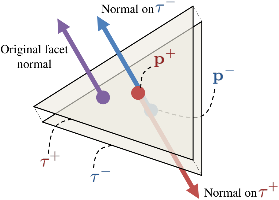
For any other third facet $\gamma\neq\tau$, $\theta_{\tau}$ and $\nabla\theta_{\mu}$ take the same value on $\gamma^{+}$ and $\gamma^{-}$. Therefore,

	$\displaystyle\int_{\gamma^{+}\cup\gamma^{-}}\theta_{\tau}(\nabla\theta_{\mu}\cdot\mathbf{n})dS$	$\displaystyle=$	$\displaystyle\int_{\gamma^{+}}\theta_{\tau}(\nabla\theta_{\mu}\cdot\mathbf{n})dS+\int_{\gamma^{-}}\theta_{\tau}(\nabla\theta_{\mu}\cdot\mathbf{n})dS$		(17)
		$\displaystyle=$	$\displaystyle\int_{\gamma^{+}}\theta_{\tau}(\nabla\theta_{\mu}\cdot\mathbf{n})dS+\int_{\gamma^{+}}\theta_{\tau}(\nabla\theta_{\mu}\cdot(-\mathbf{n}))dS$		(18)
		$\displaystyle=$	$\displaystyle 0$		(19)

where in (18) we replaced the integral over $\gamma^{-}$ with an integral over $\gamma^{+}$ with a negated surface normal. Therefore, the integral over $\partial\Omega$ is reduced to an integral over $\tau^{+}\cup\tau^{-}$, i.e.,

	$\displaystyle\int_{\partial\Omega}\theta_{\tau}(\nabla\theta_{\mu}\cdot\mathbf{n})dS$	$\displaystyle=$	$\displaystyle\sum_{\gamma\in\mathcal{M}}\int_{\gamma^{+}\cup\gamma^{-}}\theta_{\tau}(\nabla\theta_{\mu}\cdot\mathbf{n})dS$		(20)
		$\displaystyle=$	$\displaystyle\int_{\tau^{+}\cup\tau^{-}}\theta_{\tau}(\nabla\theta_{\mu}\cdot\mathbf{n})dS\ .$		(21)

Using the properties above, we arrive at:

	$\displaystyle\int_{\tau^{+}\cup\tau^{-}}\theta_{\tau}(\nabla\theta_{\mu}\cdot\mathbf{n})dS$	$\displaystyle=$	$\displaystyle\int_{\tau^{+}}(-2\pi)(\nabla\theta_{\mu}\cdot\mathbf{n})dS+\int_{\tau^{-}}(2\pi)(\nabla\theta_{\mu}\cdot\mathbf{n})dS$		(22)
		$\displaystyle=$	$\displaystyle-2\pi\int_{\tau^{+}}\nabla\theta_{\mu}\cdot\mathbf{n}\ dS+2\pi\int_{\tau^{+}}\nabla\theta_{\mu}\cdot(-\mathbf{n})\ dS$		(23)
		$\displaystyle=$	$\displaystyle-4\pi\int_{\tau^{+}}\nabla\theta_{\mu}\cdot\mathbf{n}\ dS\ .$		(24)

In summary, $Q_{ij}$ is computed as

$$Q_{ij}=\sum_{\tau\in\mathcal{P}_{i}}\sum_{\mu\in\mathcal{P}_{j}}F(\tau,\mu)$$

(25)

where

$$F(\tau,\mu)=-\frac{1}{4\pi}\int_{\mathbf{p}\in\tau^{+}}\nabla\theta_{\mu}(\mathbf{p})\cdot\mathbf{n}(\mathbf{p})\ dS\ .$$

(26)

By deriving an analytic form of $F(\tau,\mu)$ using Maple, we found that it evaluates to infinity (either positive or negative depending on relative orientation of $\tau$ and $\mu$) when some edges of $\tau$ and $\mu$ coincide geometrically. An intuitive explanation for this is that the magnitude of $\nabla\theta_{\mu}(\mathbf{p})$ becomes infinitely large when $\mathbf{p}\in\tau^{+}$ goes infinitesimally close to the edges of $\tau$ that are geometrically coinciding with the edges of $\mu$. In particular, the diagonal entries $Q_{ii}$ always evaluate to positive infinity. Although we can ignore the diagonals using (11), off-diagonal entries $Q_{ij}$ can still evaluate to infinity if some boundary edges of $\mathcal{P}_{i}$ and $\mathcal{P}_{j}$ coincide geometrically. In our experiments, we numerically evaluate the energy with a sufficiently fine discretization of $\partial\Omega$ where the finite entries in $\mathbf{Q}$ are converged.

The minimization problem in (9) is referred to as Quadratic Unconstrained Binary Optimization (QUBO). QUBO is NP-hard, and various heuristic methods exist [BHT07]. In our experiments, we take a brute force approach and exhaustively search for the optimal solution, so that we can examine the nature of our approach with small toy examples.

References

- [BHT07] Endre Boros, PeterL. Hammer, and Gabriel Tavares. Local search heuristics for quadratic unconstrained binary optimization (qubo). Journal of Heuristics, 13(2):99–132, 2007.
- [BZK04] Pavel Borodin, Gabriel Zachmann, and Reinhard Klein. Consistent normal orientation for polygonal meshes. In Proceedings of the Computer Graphics International, CGI ’04, pages 18–25, 2004.
- [JKSH13] Alec Jacobson, Ladislav Kavan, and Olga Sorkine-Hornung. Robust inside-outside segmentation using generalized winding numbers. ACM Trans. Graph., 32(4):33:1–33:12, 2013.
- [LW10] Shengjun Liu and Charlie C.L. Wang. Orienting unorganized points for surface reconstruction. Computers & Graphics, 34(3):209–218, 2010.
- [MDGD+10] Patrick Mullen, Fernando De Goes, Mathieu Desbrun, David Cohen-Steiner, and Pierre Alliez. Signing the unsigned: Robust surface reconstruction from raw pointsets. Computer Graphics Forum, 29(5):1733–1741, 2010.