跳到论文正文
W Papers独立论文阅读器 arXiv:1406.5335 论文正文 计算阅读时间 · 0%
引用这篇论文根据当前论文元数据生成,正式投稿前建议核对。


License: arXiv.org perpetual non-exclusive license
arXiv:1406.5335v1 [astro-ph.SR] 20 Jun 2014

Generalization of the noise model for time-distance helioseismology

D. Fournier Affiliation: Institut für Numerische und Angewandte Mathematik, Lotzestrasse 16-18, 37083 Göttingen, Germany Email: d.fournier@math.uni-goettingen.de    L. Gizon Affiliation: Max-Planck-Institut für Sonnensystemforschung, Justus-von-Liebig-Weg 3, 37077 Göttingen, Germany Affiliation: Institut für Astrophysik, Georg-August-Universität Göttingen, Friedrich-Hund-Platz 1, 37077 Göttingen, Germany    T. Hohage Affiliation: Institut für Numerische und Angewandte Mathematik, Lotzestrasse 16-18, 37083 Göttingen, Germany Email: d.fournier@math.uni-goettingen.de    A. C. Birch Affiliation: Max-Planck-Institut für Sonnensystemforschung, Justus-von-Liebig-Weg 3, 37077 Göttingen, Germany
Received ; accepted
Abstract

Context. In time-distance helioseismology, information about the solar interior is encoded in measurements of travel times between pairs of points on the solar surface. Travel times are deduced from the cross-covariance of the random wave field. Here we consider travel times and also products of travel times as observables. They contain information about e.g. the statistical properties of convection in the Sun.

Aims. Using the travel time definition of Gizon & Birch (2004) we derive analytic formulae for the noise covariance matrix of travel times and products of travel times.

Methods. The basic assumption of the model is that noise is the result of the stochastic excitation of solar waves, a random process which is stationary and Gaussian. We generalize the existing noise model by dropping the assumption of horizontal spatial homogeneity. Using a recurrence relation, we calculate the noise covariance matrices for the moments of order 4, 6, and 8 of the observed wave field, for the moments of order 2, 3 and 4 of the cross-covariance, and for the moments of order 2, 3 and 4 of the travel times.

Results. All noise covariance matrices depend only on the expectation value of the cross-covariance of the observed wave field. For products of travel times, the noise covariance matrix consists of three terms proportional to 1/T1/T, 1/T21/T^{2}, and 1/T31/T^{3}, where TT is the duration of the observations. For typical observation times of a few hours, the term proportional to 1/T21/T^{2} dominates and Cov​[τ1​τ2,τ3​τ4]≈Cov​[τ1,τ3]​Cov​[τ2,τ4]+Cov​[τ1,τ4]​Cov​[τ2,τ3]\textrm{Cov}[\tau_{1}\tau_{2},\tau_{3}\tau_{4}]\approx\textrm{Cov}[\tau_{1},\tau_{3}]\textrm{Cov}[\tau_{2},\tau_{4}]+\textrm{Cov}[\tau_{1},\tau_{4}]\textrm{Cov}[\tau_{2},\tau_{3}], where the τi\tau_{i} are arbitrary travel times. This result is confirmed for p1p_{1} travel times by Monte Carlo simulations and comparisons with SDO/HMI observations.

Conclusions. General and accurate formulae have been derived to model the noise covariance matrix of helioseismic travel times and products of travel times. These results could easily be generalized to other methods of local helioseismology, such as helioseismic holography and ring diagram analysis.

Key Words.
Sun: helioseismology – Sun: oscillations – Sun: granulation – convection – methods: statistical – methods: data analysis

1 Introduction

The purpose of time-distance helioseismology (Duvall et al. 1993; Gizon & Birch 2005, and references therein) is to infer the subsurface structure and dynamics of the Sun using spatial-temporal correlations of the random wave field observed at the solar surface. Wave travel times between pairs of points (denoted τ\tau) are measured from the cross-covariance function. Wave speed perturbations and vector flows are then obtained by inversion of the travel times (e.g. Kosovichev (1996); Jackiewicz et al. (2012)). Such inversions require knowledge of the noise covariance matrix Cov[τ,τ\tau,\tau]. Typically, noise is very high and strong correlations exist among travel times. Gizon & Birch (2004) studied the noise properties of travel times and derived a simple noise model that successfully explains the observations. The model is based on the assumption that the stochastic noise is stationary and horizontally spatially homogeneous, as a result of the excitation of waves by turbulent convection. In addition to time-distance helioseismology, this noise model has found applications in direct modeling inversions (Woodard 2006; Woodard 2009) and ring-diagram analysis (Birch et al. 2007).

Time-distance helioseismology has been successfully applied to map flow velocities, vjv_{j}, at supergranulation scales (Kosovichev 1996; Duvall Jr. & Gizon 2000; Gizon et al. 2001; Jackiewicz et al. 2008). The statistical properties of convection can further be studied by computing horizontal averages of the turbulent velocities. For example, Duvall Jr. & Gizon (2000); Gizon et al. (2010) showed that the horizontal divergence and the vertical vorticity of the flows are correlated through the influence of the Coriolis force on convection. It would be highly desirable to extract additional properties of the turbulent velocities, for example the (anisotropic) Reynolds stresses ⟨vi​vj⟩\langle v_{i}v_{j}\rangle that control the global dynamics of the Sun (Kitchatinov & Rüdiger 2005, differential rotation and meridional circulation, see). The noise associated with such measurement involves the fourth order moments of the travel times, Cov​[τ​τ,τ​τ]\textrm{Cov}[\tau\tau,\tau\tau].

Alternatively, we would like to consider spatial averages of products of travel times ⟨τ​τ⟩\langle\tau\tau\rangle as the fundamental data from which to infer the Reynolds stresses (or other second-order moments of turbulence). Spatial averages are meaningful when turbulent flows are horizontally homogeneous over the averaging region. Inversions of average products of travel times are desirable since input data are fewer and less noisy. Once again, we need to know the noise covariance matrix Cov​[⟨τ​τ⟩,⟨τ​τ⟩]\textrm{Cov}[\langle\tau\tau\rangle,\langle\tau\tau\rangle] in order to perform the inversion.

In this paper, we study the noise properties of travel times and products of travel times. In Section 2, the definitions for the cross-covariance function and the travel times are given. Section 3 presents the assumptions of the noise model generalizing the model of Gizon & Birch (2004). In Section 4 and in the Appendix, we derive analytical formulae for the noise covariance matrices of travel times and products of travel times. These formulae are confirmed in Section 5 by comparison to numerical Monte Carlo simulations and to SDO/HMI observations. The effects of horizontal spatial averaging are considered in Section 6.

2 Observables: cross-covariance function, travel times, and products of travel times

The fundamental observation in helioseismology is the filtered line-of-sight Doppler velocity ϕ⁡(𝐱,t)\phi(\mathbf{x},t) at points 𝐱\mathbf{x} on the surface of the Sun and at times tt. The filter acts by multiplication in the Fourier domain. In this paper we will only consider the p1−p_{1}-ridge filter as an example. Note that all the results presented in this paper do not depend on the choice of the filter. The signal ϕ⁡(𝐱,t)\phi(\mathbf{x},t) is recorded over a duration time T=(2​N+1)​htT=(2N+1)h_{t} where hth_{t} is the temporal resolution at observation times tn=n​htt_{n}=nh_{t} for n=−N,…,Nn=-N,\dots,N. The observed wavefield during the observation time TT is denoted ϕT\phi_{T}. We have ϕT​(𝐱,t)=ϕ⁡(𝐱,t)​WinT⁡(t)\phi_{T}(\mathbf{x},t)=\phi(\mathbf{x},t)\Win_{T}(t) where WinT\Win_{T} is a window function (equal to 1 if |t|≤T/2\left|t\right|\leq T/2 and 0 otherwise).

Helioseismic analysis is performed in Fourier space. Let us define the temporal Fourier transform of ϕT\phi_{T} by

ϕT​(𝐱,ω):=ht2​π​∑n=−NNϕ⁡(𝐱,tn)​exp⁡(i​ω​tn).\phi_{T}(\mathbf{x},\omega):=\frac{h_{t}}{2\pi}\sum_{n=-N}^{N}\phi(\mathbf{x},t_{n})\exp(i\omega t_{n}).

The frequencies ω\omega are treated as continuous variables in the remainder of this paper in order to be able to take into account the frequency correlations (see Section 3.3). The cross-covariance function between two points at the surface of the Sun is a multiplication in the Fourier domain (Duvall et al. 1993)

C⁡(𝐱1,𝐱2,ω)=2​πT​ϕT∗​(𝐱1,ω)​ϕT​(𝐱2,ω).C(\mathbf{x}_{1},\mathbf{x}_{2},\omega)=\frac{2\pi}{T}\phi_{T}^{\ast}(\mathbf{x}_{1},\omega)\phi_{T}(\mathbf{x}_{2},\omega). (1)

Working in Fourier space is faster (and easier). In the time-domain the cross-covariance becomes

C⁡(𝐱1,𝐱2,tn):=12​N+1​∑j=max⁡(−N,−N−n)min⁡(N,N−n)ϕ⁡(𝐱1,tj)​ϕ​(𝐱2,tj+n).C(\mathbf{x}_{1},\mathbf{x}_{2},t_{n}):=\frac{1}{2N+1}\sum_{j=\max(-N,-N-n)}^{\min(N,N-n)}\phi(\mathbf{x}_{1},t_{j})\phi(\mathbf{x}_{2},t_{j+n}). (2)

where tnt_{n} is the correlation time lag.

Cross-covariances are the basic data to compute the travel times. We denote τ+​(𝐱1,𝐱2)\tau_{+}(\mathbf{x}_{1},\mathbf{x}_{2}) the travel time for a wave packet traveling from point 𝐱1\mathbf{x}_{1} to point 𝐱2\mathbf{x}_{2} and τ−​(𝐱1,𝐱2)\tau_{-}(\mathbf{x}_{1},\mathbf{x}_{2}) the travel time for a wave packet traveling from 𝐱2\mathbf{x}_{2} to 𝐱1\mathbf{x}_{1}. In the limit discussed by Gizon & Birch (2004) the incremental travel times can be measured from the estimated cross-covariance using

τ±(𝐱1,𝐱2):=ht∑n=−NN\displaystyle\tau_{\pm}(\mathbf{x}_{1},\mathbf{x}_{2}):=h_{t}\sum_{n=-N}^{N} W±(𝐱1,𝐱2,tn)×\displaystyle W_{\pm}(\mathbf{x}_{1},\mathbf{x}_{2},t_{n})\times
(C⁡(𝐱1,𝐱2,tn)−Cref​(𝐱1,𝐱2,tn))\displaystyle\left(C(\mathbf{x}_{1},\mathbf{x}_{2},t_{n})-C^{\textrm{ref}}(\mathbf{x}_{1},\mathbf{x}_{2},t_{n})\right) (3)

where CrefC^{\textrm{ref}} is a deterministic reference cross-covariance coming from spatial averaging or from a solar model and the weight function W±W_{\pm} are defined as

W±​(𝐱1,𝐱2,t):=∓f(±t)∂tCref(𝐱1,𝐱2,t)ht​∑nf⁡(±tn)​[∂tCref​(𝐱1,𝐱2,tn)]2W_{\pm}(\mathbf{x}_{1},\mathbf{x}_{2},t):=\frac{\mp f(\pm t)\partial_{t}C^{\textrm{ref}}(\mathbf{x}_{1},\mathbf{x}_{2},t)}{h_{t}\sum_{n}f(\pm t_{n})[\partial_{t}C^{\textrm{ref}}(\mathbf{x}_{1},\mathbf{x}_{2},t_{n})]^{2}} (4)

with ff a window function used to select an interval of time around the first arrival time of the wave packet (for example, a cut-off function). Notice that for spatially homogeneous noise we generally choose that Cref​(𝐱1,𝐱2,t)=Cref​(𝐱2−𝐱1,t)C^{\textrm{ref}}(\mathbf{x}_{1},\mathbf{x}_{2},t)=C^{\textrm{ref}}(\mathbf{x}_{2}-\mathbf{x}_{1},t) which implies that W⁡(𝐱1,𝐱2,t)=W⁡(𝐱2−𝐱1,t)W(\mathbf{x}_{1},\mathbf{x}_{2},t)=W(\mathbf{x}_{2}-\mathbf{x}_{1},t). However, this assumption is not necessary in the remainder of this paper.

We write τα\tau_{\alpha} where the subscript

α∈{+,−,diff,mean}\alpha\in\{+,-,\textrm{diff},\textrm{mean}\}

denotes the type of travel time and the corresponding weight function WαW_{\alpha}. The mean and difference travel times τdiff\tau_{\textrm{diff}} and τmean\tau_{\textrm{mean}} can be obtained from the one way travel times by τdiff=τ+−τ−\tau_{\textrm{diff}}=\tau_{+}-\tau_{-} and τmean=(τ++τ−)/2\tau_{\textrm{mean}}=(\tau_{+}+\tau_{-})/2.

In this paper, we are interested in the noise covariance matrix for travel times τα1​(𝐱1,𝐱2)\tau_{\alpha_{1}}(\mathbf{x}_{1},\mathbf{x}_{2}) and products of travel times τα1​(𝐱1,𝐱2)​τα2​(𝐱3,𝐱4)\tau_{\alpha_{1}}(\mathbf{x}_{1},\mathbf{x}_{2})\tau_{\alpha_{2}}(\mathbf{x}_{3},\mathbf{x}_{4}) where τ\tau is defined by Eq. (3). To simplify the notations, let

τ1:=τα1​(𝐱1,𝐱2),τ2:=τα2​(𝐱3,𝐱4),\tau_{1}:=\tau_{\alpha_{1}}(\mathbf{x}_{1},\mathbf{x}_{2}),\quad\tau_{2}:=\tau_{\alpha_{2}}(\mathbf{x}_{3},\mathbf{x}_{4}),
and more generally ​τi:=ταi​(𝐱2​i−1,𝐱2​i).\textrm{and more generally }\tau_{i}:=\tau_{\alpha_{i}}(\mathbf{x}_{2i-1},\mathbf{x}_{2i}). (5)

3 Generalization of the noise model

3.1 Assumptions

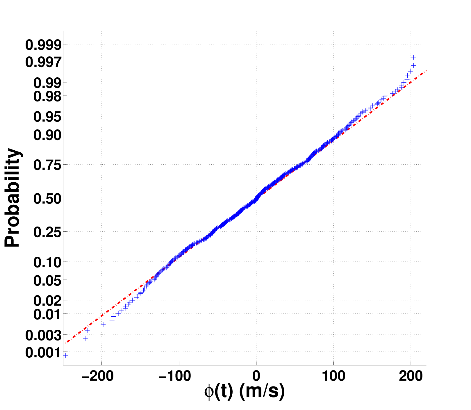
The basic assumption of the noise model is the following: The observations at the relevant spatial points 𝐱1,…,𝐱M\mathbf{x}_{1},\dots,\mathbf{x}_{M} are described by a vector-valued stationary Gaussian time series (ϕ⁡(𝐱𝟏,𝐭𝐧),…,ϕ⁡(𝐱𝐌,𝐭𝐧))\mathbf{(\phi(\mathbf{x}_{1},t_{n}),\dots,\phi(\mathbf{x}_{M},t_{n}))}. For the sake of simplicity, we can also assume without loss of generality that 𝔼⁡[ϕ⁡(𝐱m,tn)]=0\mathbb{E}\left[\phi(\mathbf{x}_{m},t_{n})\right]=0 at each 𝐱m\mathbf{x}_{m} for all n∈ℤn\in\mathbb{Z}. This model is valid in the quiet Sun (away from evolving active regions) but does not assume that the noise is spatially homogeneous contrary to the model of Gizon & Birch (2004) as detailed in Section 3.2. This assumption is supported by the observed distribution of the HMI Doppler velocity: Figure 1 shows the probability density of the filtered line-of-sight velocity. For a Gaussian distribution, the data should line up along a straight line. We can see a very good agreement for probabilities betweeen 5%5\% and 95%95\%. The deviations in the tail of the plot (for probabilities smaller than 5%5\%) may be due to statistical errors (as we have less realisations for these events).
Refer to caption
Figure 1: Probability density plot representing the filtered line-of-sight velocity ϕ⁡(t)\phi(t) for a p1−p_{1}-ridge with an observation time T=8T=8 h. For Gaussian observations, all data should be on a straight line.

One may also replace the spatial points by some spatial averages. Such averages are often used to improve the signal-to-noise ratio We will denote C¯\overline{C} the expectation value of the cross-covariance

C¯​(𝐱a,𝐱b,ω)=𝔼⁡[C⁡(𝐱a,𝐱b,ω)]=2​πT​𝔼​[ϕT∗​(𝐱a,ω)​ϕT​(𝐱b,ω)].\overline{C}(\mathbf{x}_{a},\mathbf{x}_{b},\omega)=\mathbb{E}\left[C(\mathbf{x}_{a},\mathbf{x}_{b},\omega)\right]=\frac{2\pi}{T}\mathbb{E}\left[\phi_{T}^{\ast}(\mathbf{x}_{a},\omega)\phi_{T}(\mathbf{x}_{b},\omega)\right]. (6)

3.2 Independance of the geometry

Gizon & Birch (2004) assumed that the observations ϕ⁡(𝐱i​j,tn)\phi(\mathbf{x}_{ij},t_{n}) are given on a Cartesian grid {𝐱i​j}\{\mathbf{x}_{ij}\} by an approximately flat patch of the Sun’s surface. The discrete Fourier transform of the finite dimensional signal was assumed to be of the form

ϕ⁡(𝐤i​j,ωl)=𝒫⁡(𝐤i​j,ωl)​𝒩i​j​l\phi({\bf k}_{ij},\omega_{l})=\sqrt{\mathcal{P}({\bf k}_{ij},\omega_{l})}\mathcal{N}_{ijl} (7)

where 𝒫{\mathcal{P}} is the power spectrum, ωl:=2​π​l/T\omega_{l}:=2\pi l/T, and 𝒩i​j​l\mathcal{N}_{ijl} are complex independent and identically distributed Gaussian variables with zero-mean and unit variance. In this case, the frequency correlations were ignored and

2​πT​𝔼​[ϕ∗​(𝐱a,ωj)​ϕ​(𝐱b,ωl)]=δj​l​C¯G​B​(𝐱b−𝐱a,ωl)\frac{2\pi}{T}\mathbb{E}\left[\phi^{\ast}(\mathbf{x}_{a},\omega_{j})\phi(\mathbf{x}_{b},\omega_{l})\right]=\delta_{jl}\overline{C}_{GB}(\mathbf{x}_{b}-\mathbf{x}_{a},\omega_{l}) (8)

was assumed. We have denoted C¯G​B\overline{C}_{GB} the expectation value of the cross-covariance used by Gizon & Birch (2004). Our assumption is more general as it does not require a planar geometry and allows a natural treatment of spatially averaged quantities. It means that all our results are valid in any geometry and it is in particular the case for the results presented in Gizon & Birch (2004).

3.3 On frequency correlations

As the observation time TT is finite, the discrete Fourier transforms ϕT​(𝐱,ωj)\phi_{T}(\mathbf{x},\omega_{j}) and ϕT​(𝐱,ωl)\phi_{T}(\mathbf{x},\omega_{l}) for j≠lj\neq l are no longer uncorrelated because of the window function. The necessity of a correction term for finite TT was discussed, but not further analyzed in Gizon & Birch (2004). It turns out that there is an explicit formula for this correction term in terms of the periodic Hilbert transform of C¯\overline{C} and a smoothed version of C¯\overline{C}. The exact formulation is given in Appendix A where it is also shown that the error made by considering a finite observation time can be bounded

supj,l|2​πT𝔼[ϕT∗(𝐱a,ωj)ϕT(𝐱b,ωl)]−δj​lC¯G​B(𝐱b−𝐱a,ωl)]|\displaystyle\sup_{j,l}\left|\frac{2\pi}{T}\mathbb{E}\left[\phi_{T}^{\ast}(\mathbf{x}_{a},\omega_{j})\phi_{T}(\mathbf{x}_{b},\omega_{l})\right]-\delta_{jl}\overline{C}_{GB}(\mathbf{x}_{b}-\mathbf{x}_{a},\omega_{l})]\right|
≤ht4​T​|∑k=−2​N2​N|tk|​C¯​(𝐱a,𝐱b,tk)|.\displaystyle\leq\frac{h_{t}}{4T}\left|\sum_{k=-2N}^{2N}\left|t_{k}\right|\overline{C}(\mathbf{x}_{a},\mathbf{x}_{b},t_{k})\right|. (9)

Note that the right hand side of (9) depends only on TT and on a quantity depending on the correlation length of the waves. This can be better seen using an analytic cross-covariance given by a Lorentzian of the form

C¯​(𝐱,𝐱,ω)=C01+(ω−ω0)2/γ2\overline{C}(\mathbf{x},\mathbf{x},\omega)=\frac{C_{0}}{1+(\omega-\omega_{0})^{2}/\gamma^{2}} (10)

where γ\gamma is the half width at half maximum of the Lorentzian centered at a frequency ω0\omega_{0}. In this case, one can check that the bound in Eq. (9) is equal to 1/(4​π2​γ​T)1/(4\pi^{2}\gamma T). Therefore the correlations between frequencies should only be neglected when this bound is small, i.e. the observation time is long enough to represent correctly the mode.

As the covariance between travel times is known to be also of order 1/T1/T (Gizon & Birch 2004), it is legitimate to wonder if the frequency correlations should be taken into account. It is shown below (see Eq. (13)) that considering frequency correlations will only lead to additional terms of order 1/T21/T^{2} that can be neglected for long observation times.

4 Model noise covariances

In this section and Appendices B–E we present explicit formulae for the covariance matrices of cross-covariances CC, travel times τ\tau and products of cross-covariances or travel-times:

  • •

    Cov​[τ1,τ2]\textrm{Cov}[\tau_{1},\tau_{2}] and Cov​[C1,C2]\textrm{Cov}[C_{1},C_{2}] which are linked to the fourth order moment of ϕT\phi_{T},

  • •

    Cov​[τ1​τ2,τ3]\textrm{Cov}[\tau_{1}\tau_{2},\tau_{3}] and Cov​[C1​C2,C3]\textrm{Cov}[C_{1}C_{2},C_{3}] which requires the knowledge of the sixth order moment of ϕT\phi_{T} and is necessary to compute the moment of order four of τ\tau and CC,

  • •

    Cov​[τ1​τ2,τ3​τ4]\textrm{Cov}[\tau_{1}\tau_{2},\tau_{3}\tau_{4}] and Cov​[C1​C2,C3​C4]\textrm{Cov}[C_{1}C_{2},C_{3}C_{4}] which depend on the eighth order moment of ϕT\phi_{T}.

For the covariance between two complex random variables XX and YY we will use the convention

Cov​[X,Y]=𝔼⁡[X​Y∗]−𝔼⁡[X]​𝔼​[Y∗].\textrm{Cov}[X,Y]=\mathbb{E}\left[XY^{\ast}\right]-\mathbb{E}\left[X\right]\mathbb{E}\left[Y^{\ast}\right]. (11)

In particular, as the mean value of the observables is zero, we have C¯​(𝐱1,𝐱2,ω)=2​πT​Cov​[ϕT​(𝐱2,ω),ϕT​(𝐱1,ω)].\overline{C}(\mathbf{x}_{1},\mathbf{x}_{2},\omega)=\frac{2\pi}{T}\textrm{Cov}[\phi_{T}(\mathbf{x}_{2},\omega),\phi_{T}(\mathbf{x}_{1},\omega)].

We will show that all moments of cross-covariance functions depend on C¯\overline{C} only. Because the travel time measurement procedure is linear in CC, the moments of the travel-times can be expressed in terms of C¯\overline{C} and of the weight functions WiW_{i} (see Eq. (4)).

4.1 Covariance matrix for CC and travel times

As a first step, we show in Appendix C that the covariance between two cross-correlations is given by

(T2​π)2\displaystyle\left(\frac{T}{2\pi}\right)^{2} Cov​[C⁡(𝐱1,𝐱2,ω1),C⁡(𝐱3,𝐱4,ω2)]=\displaystyle\textrm{Cov}[C(\mathbf{x}_{1},\mathbf{x}_{2},\omega_{1}),C(\mathbf{x}_{3},\mathbf{x}_{4},\omega_{2})]=
𝔼⁡[ϕ∗​(𝐱1,ω1)​ϕ​(𝐱3,ω2)]​𝔼​[ϕ⁡(𝐱2,ω1)​ϕ∗​(𝐱4,ω2)]\displaystyle\mathbb{E}[\phi^{\ast}(\mathbf{x}_{1},\omega_{1})\phi(\mathbf{x}_{3},\omega_{2})]\;\mathbb{E}[\phi(\mathbf{x}_{2},\omega_{1})\phi^{\ast}(\mathbf{x}_{4},\omega_{2})] (12)
+𝔼⁡[ϕ∗​(𝐱1,ω1)​ϕ∗​(𝐱4,ω2)]​𝔼​[ϕ⁡(𝐱2,ω1)​ϕ​(𝐱3,ω2)].\displaystyle+\mathbb{E}[\phi^{\ast}(\mathbf{x}_{1},\omega_{1})\phi^{\ast}(\mathbf{x}_{4},\omega_{2})]\;\mathbb{E}[\phi(\mathbf{x}_{2},\omega_{1})\phi(\mathbf{x}_{3},\omega_{2})].

For a comparison with and a small correction to the corresponding formula in Gizon & Birch (2004) we refer to Appendix B. The covariance between two travel times is given by

Cov[τ1,τ2]=(2​π)3T∫−π/htπ/htdωWα1∗(𝐱1,𝐱2,ω)×\displaystyle\textrm{Cov}[\tau_{1},\tau_{2}]=\frac{(2\pi)^{3}}{T}\int_{-\pi/h_{t}}^{\pi/h_{t}}d\omega W_{\alpha_{1}}^{\ast}(\mathbf{x}_{1},\mathbf{x}_{2},\omega)\times
(Wα2​(𝐱3,𝐱4,ω)​C¯​(𝐱1,𝐱3,ω)​C¯​(𝐱4,𝐱2,ω)CLOSE\displaystyle\quad\Bigl(W_{\alpha_{2}}(\mathbf{x}_{3},\mathbf{x}_{4},\omega)\overline{C}(\mathbf{x}_{1},\mathbf{x}_{3},\omega)\overline{C}(\mathbf{x}_{4},\mathbf{x}_{2},\omega) (13)
OPEN+Wα2∗​(𝐱3,𝐱4,ω)​C¯​(𝐱1,𝐱4,ω)​C¯​(𝐱3,𝐱2,ω))+X2T2+𝒪⁡(1Tm+1)\displaystyle\quad+W_{\alpha_{2}}^{\ast}(\mathbf{x}_{3},\mathbf{x}_{4},\omega)\overline{C}(\mathbf{x}_{1},\mathbf{x}_{4},\omega)\overline{C}(\mathbf{x}_{3},\mathbf{x}_{2},\omega)\Bigr)+\frac{X_{2}}{T^{2}}+{\mathcal{O}}\left(\frac{1}{T^{m+1}}\right)

where 𝒪⁡(1/Tm+1){\mathcal{O}}\left(1/T^{m+1}\right) means that the additional terms decay at least as 1/Tm+11/T^{m+1} (mm corresponds to the regularity, i.e. the number of derivatives of the functions C¯\overline{C} and WW). A good agreement between the leading order term in this formula and SOHO MDI measurements was found by Gizon & Birch (2004). An explicit formula for the second order term X2X_{2} is derived in Appendices B and D. If the observation time TT is so small that X2/T2X_{2}/T^{2} cannot be neglected, X2X_{2} can easily be evaluated numerically.

4.2 Covariance matrix for products of travel times

In this section, we are interested in the covariance matrix for the travel times correlations i.e. to evaluate the quantity

Cov​[τ1​(𝐱1,𝐱2)​τ2​(𝐱3,𝐱4),τ3​(𝐱5,𝐱6)​τ4​(𝐱7,𝐱8)].\textrm{Cov}[\tau_{1}(\mathbf{x}_{1},\mathbf{x}_{2})\tau_{2}(\mathbf{x}_{3},\mathbf{x}_{4}),\tau_{3}(\mathbf{x}_{5},\mathbf{x}_{6})\tau_{4}(\mathbf{x}_{7},\mathbf{x}_{8})]. (14)

This quantity is the most general we can evaluate for velocity correlations. It will be helpful to derive all the formulae in more specific frameworks. In general this quantity depends on the eight points 𝐱i\mathbf{x}_{i} but it is of course possible to look at simpler cases. For example, we may be interested in the correlations between a East-West (EW) and North-South (NS) travel time as presented in Figure 4. This quantity can give us informations about the correlations between the velocities vxv_{x} and vyv_{y}, velocities in the E​WEW and N​SNS directions respectively.

The formula for the product of cross-covariances is given in Appendix E (Eq. (65)) and will not be discussed in the text where we will focus on products of travel times. In Appendix E, we derive the general formula for Eq. (14)

Cov​[τ1​τ2,τ3​τ4]=1T​Z1+1T2​Z2+1T3​Z3+𝒪⁡(1T4)\textrm{Cov}[\tau_{1}\tau_{2},\tau_{3}\tau_{4}]=\frac{1}{T}Z_{1}+\frac{1}{T^{2}}Z_{2}+\frac{1}{T^{3}}Z_{3}+{\mathcal{O}}\left(\frac{1}{T^{4}}\right) (15)

where Z1Z_{1}, Z2Z_{2} and Z3Z_{3} are given by Eqs. (16), (18) and (20) and will be detailed later after some general remarks on this formula. An important point is that all the terms in ZiZ_{i} depend only on C¯\overline{C} and on the weight functions WW. Thus, it is possible to estimate directly the noise covariance matrix via this formula instead of performing a large number of Monte-Carlo simulations. This strategy is much more efficient as we will see in Section 5.3 where we demonstrate the rate of convergence of the stochastic simulations.

The terms on the right hand side of the general formula Eq. (15) are of different orders with respect to the observation time. The behaviour of these terms is studied in Section 5.6.2.

Let us now give the expressions for the different terms ZiZ_{i} in Eq. (15). The term of order T−1T^{-1} is given by (for details, see Appendix E):

1T​Z1=\displaystyle\frac{1}{T}Z_{1}= τ¯2​(τ¯4​Cov​[τ1,τ3]+τ¯3​Cov​[τ1,τ4])\displaystyle\overline{\tau}_{2}\Bigl(\overline{\tau}_{4}\textrm{Cov}[\tau_{1},\tau_{3}]+\overline{\tau}_{3}\textrm{Cov}[\tau_{1},\tau_{4}]\Bigr)
+τ¯1​(τ¯4​Cov​[τ2,τ3]+τ¯3​Cov​[τ2,τ4])\displaystyle+\overline{\tau}_{1}\Bigl(\overline{\tau}_{4}\textrm{Cov}[\tau_{2},\tau_{3}]+\overline{\tau}_{3}\textrm{Cov}[\tau_{2},\tau_{4}]\Bigr) (16)

where the covariance between two travel times is given by Eq. (13) and τ¯j\overline{\tau}_{j} is the expectation value of the travel time τj\tau_{j}, for example,

τ¯1=∫−π/htπ/htdωW1∗(𝐱1,𝐱2,ω)(C¯(𝐱1,𝐱2,ω)−Cref(𝐱1,𝐱2,ω)).\overline{\tau}_{1}=\int_{-\pi/h_{t}}^{\pi/h_{t}}d\omega W_{1}^{\ast}(\mathbf{x}_{1},\mathbf{x}_{2},\omega)\left(\overline{C}(\mathbf{x}_{1},\mathbf{x}_{2},\omega)-C^{\textrm{ref}}(\mathbf{x}_{1},\mathbf{x}_{2},\omega)\right). (17)

As CrefC^{\textrm{ref}} and C¯\overline{C} are generally close or even equal it is possible that this quantity is close to 0 or even exactly 0. This simplification is discussed in Section 4.3. Note that the time dependence (in T−1T^{-1}) in Eq. (16) is hidden on the right hand side in the covariance betweeen two travel times (cf. Eq. (13)).

The term of order T−2T^{-2} is given by:

1T2​Z2=\displaystyle\frac{1}{T^{2}}Z_{2}= Cov​[τ1,τ3]​Cov​[τ2,τ4]+Cov​[τ1,τ4]​Cov​[τ2,τ3]\displaystyle\textrm{Cov}[\tau_{1},\tau_{3}]\textrm{Cov}[\tau_{2},\tau_{4}]+\textrm{Cov}[\tau_{1},\tau_{4}]\textrm{Cov}[\tau_{2},\tau_{3}]
−τ¯1​(Cov​[τ2,τ3​τ4]+τ¯3​Cov​[τ2,τ4]+τ¯4​Cov​[τ2,τ3])\displaystyle-\overline{\tau}_{1}\left(\textrm{Cov}[\tau_{2},\tau_{3}\tau_{4}]+\overline{\tau}_{3}\textrm{Cov}[\tau_{2},\tau_{4}]+\overline{\tau}_{4}\textrm{Cov}[\tau_{2},\tau_{3}]\right)
−τ¯2​(Cov​[τ1,τ3​τ4]+τ¯3​Cov​[τ1,τ4]+τ¯4​Cov​[τ1,τ3])\displaystyle-\overline{\tau}_{2}\left(\textrm{Cov}[\tau_{1},\tau_{3}\tau_{4}]+\overline{\tau}_{3}\textrm{Cov}[\tau_{1},\tau_{4}]+\overline{\tau}_{4}\textrm{Cov}[\tau_{1},\tau_{3}]\right)
−τ¯3​(Cov​[τ1​τ2,τ4]+τ¯1​Cov​[τ2,τ4]+τ¯2​Cov​[τ1,τ4])\displaystyle-\overline{\tau}_{3}\left(\textrm{Cov}[\tau_{1}\tau_{2},\tau_{4}]+\overline{\tau}_{1}\textrm{Cov}[\tau_{2},\tau_{4}]+\overline{\tau}_{2}\textrm{Cov}[\tau_{1},\tau_{4}]\right)
−τ¯4​(Cov​[τ1​τ2,τ3]+τ¯1​Cov​[τ2,τ3]+τ¯2​Cov​[τ1,τ3])\displaystyle-\overline{\tau}_{4}\left(\textrm{Cov}[\tau_{1}\tau_{2},\tau_{3}]+\overline{\tau}_{1}\textrm{Cov}[\tau_{2},\tau_{3}]+\overline{\tau}_{2}\textrm{Cov}[\tau_{1},\tau_{3}]\right) (18)

where the covariance involving three travel times is given in the Appendix E.2 by Eq. (90) and the one between two travel times by Eq. (13). As we will see in Section 5 the first line of this term is dominant in most of the applications.

To write down the term Z3Z_{3} of order T−3T^{-3} we introduce a function Γα1,α2\Gamma_{\alpha_{1},\alpha_{2}} such that

Cov[τ1,τ2]=(2​π)3T∫−π/htπ/htdωΓα1,α2(𝐱1,𝐱2,𝐱3,𝐱4,ω)+𝒪(T−2),\textrm{Cov}[\tau_{1},\tau_{2}]=\frac{(2\pi)^{3}}{T}\int_{-\pi/h_{t}}^{\pi/h_{t}}d\omega\ \Gamma_{\alpha_{1},\alpha_{2}}(\mathbf{x}_{1},\mathbf{x}_{2},\mathbf{x}_{3},\mathbf{x}_{4},\omega)+\mathcal{O}(T^{-2}),

i.e. according to Eq. (13)

Γα1,α2​(𝐱1,𝐱2CLOSE,\displaystyle\Gamma_{\alpha_{1},\alpha_{2}}(\mathbf{x}_{1},\mathbf{x}_{2}, OPEN𝐱3,𝐱4,ω)=\displaystyle\mathbf{x}_{3},\mathbf{x}_{4},\omega)=
Wα1∗​(𝐱1,𝐱2)​(CLOSE\displaystyle W_{\alpha_{1}}^{\ast}(\mathbf{x}_{1},\mathbf{x}_{2})\Bigl( Wα2​(𝐱3,𝐱4,ω)​C¯​(𝐱1,𝐱3,ω)​C¯​(𝐱4,𝐱2,ω)\displaystyle W_{\alpha_{2}}(\mathbf{x}_{3},\mathbf{x}_{4},\omega)\overline{C}(\mathbf{x}_{1},\mathbf{x}_{3},\omega)\overline{C}(\mathbf{x}_{4},\mathbf{x}_{2},\omega)
OPEN+Wα2∗​(𝐱3,𝐱4,ω)​C¯​(𝐱1,𝐱4,ω)​C¯​(𝐱3,𝐱2,ω)).\displaystyle+W_{\alpha_{2}}^{\ast}(\mathbf{x}_{3},\mathbf{x}_{4},\omega)\overline{C}(\mathbf{x}_{1},\mathbf{x}_{4},\omega)\overline{C}(\mathbf{x}_{3},\mathbf{x}_{2},\omega)\Bigr). (19)

Then the term of order T−3T^{-3} is given by

Z3=(2​π)7T3∑μ∈ℳ∫−π/htπ/htdωΓα1,αμ1(𝐱1,𝐱2,𝐱μ1,𝐱μ2,ω)×Γαμ3,αμ5​(𝐱μ3,𝐱μ4,𝐱μ5,𝐱μ6,ω)\displaystyle\begin{aligned} Z_{3}=\frac{(2\pi)^{7}}{T^{3}}\sum_{\mu\in{\mathcal{M}}}\int_{-\pi/h_{t}}^{\pi/h_{t}}d\omega&\Gamma_{\alpha_{1},\alpha_{\mu_{1}}}(\mathbf{x}_{1},\mathbf{x}_{2},\mathbf{x}_{\mu_{1}},\mathbf{x}_{\mu_{2}},\omega)\times\\ &\Gamma_{\alpha_{\mu_{3}},\alpha_{\mu_{5}}}(\mathbf{x}_{\mu_{3}},\mathbf{x}_{\mu_{4}},\mathbf{x}_{\mu_{5}},\mathbf{x}_{\mu_{6}},\omega)\end{aligned} (20)

where μ={μ1,μ2,⋯,μ6}\mu=\{\mu_{1},\mu_{2},\cdots,\mu_{6}\} and the subset ℳ{\mathcal{M}} contains all μ\mu satisfying

{μ1+1<μ2​ if ​μ1​ odd μ1<μ2​ if ​μ1​ even μ3<μ4<μ5<μ6μ1,…​μ6∈3,…,8.\left\{\begin{array}[]{llll}\mu_{1}+1<\mu_{2}\textrm{ if }\mu_{1}\textrm{ odd }\\ \mu_{1}<\mu_{2}\textrm{ if }\mu_{1}\textrm{ even }\\ \mu_{3}<\mu_{4}<\mu_{5}<\mu_{6}\\ {\mu_{1},\ldots\mu_{6}}\in{3,\ldots,8}.\end{array}\right. (21)

ℳ{\mathcal{M}} contains 12 elements, so the term Z3Z_{3} consists in a sum of 12 terms containing a product of the functions Γ\Gamma defined by Eq. (19).

4.3 Important special cases

4.3.1 Case Cref=C¯C^{\textrm{ref}}=\overline{C}

As CrefC^{\textrm{ref}} is generally choosen as an average value of the observations, we have Cref=C¯C^{\textrm{ref}}=\overline{C} or at least Cref≈C¯C^{\textrm{ref}}\approx\overline{C}. If there is equality then we can simplify the formula given in the previous section because τ¯=0\overline{\tau}=0. It follows that the term Z1Z_{1} is zero as are some elements of Z2Z_{2}. Denoting by Z~2\tilde{Z}_{2} the value of Z2Z_{2} when Cref=C¯C^{\textrm{ref}}=\overline{C}, we have

1T2​Z~2=Cov​[τ1,τ3]​Cov​[τ2,τ4]+Cov​[τ1,τ4]​Cov​[τ2,τ3].\frac{1}{T^{2}}\tilde{Z}_{2}=\textrm{Cov}[\tau_{1},\tau_{3}]\textrm{Cov}[\tau_{2},\tau_{4}]+\textrm{Cov}[\tau_{1},\tau_{4}]\textrm{Cov}[\tau_{2},\tau_{3}]. (22)

This term is of order T−2T^{-2} as each of the covariance in Eq. (22) are of order T−1T^{-1}. The noise covariance matrix is now given by the sum of two terms of order T−2T^{-2} and T−3T^{-3}:

Cov​[τ1​τ2,τ3​τ4]\displaystyle\textrm{Cov}[\tau_{1}\tau_{2},\tau_{3}\tau_{4}] =1T2​Z~2+1T3​Z3+𝒪⁡(1T4).\displaystyle=\frac{1}{T^{2}}\tilde{Z}_{2}+\frac{1}{T^{3}}Z_{3}+{\mathcal{O}}\left(\frac{1}{T^{4}}\right). (23)

4.3.2 Case Cref≈C¯C^{\textrm{ref}}\approx\overline{C}

Suppose now that we do not have equality but Cref=(1+ϵ)​C¯C^{\textrm{ref}}=(1+\epsilon)\overline{C} where ϵ\epsilon is a small parameter measuring the difference between the reference cross-covariance and their expectation value. In this case Z1Z_{1} is of order ϵ2\epsilon^{2} and the terms that cancelled out previously in Z2Z_{2} when Cref=C¯C^{\textrm{ref}}=\overline{C} are of order ϵ\epsilon. The numerical tests from Section 5.6.1 will confirm that these terms of order ϵ\epsilon and ϵ2\epsilon^{2} can be neglected so that Eq. (23) can be used even if we just have Cref≈C¯C^{\textrm{ref}}\approx\overline{C}.

4.3.3 Simplified formula

We have now defined all the terms involved in Eq. (15) to compute the covariance of a product of travel times. As one term is of order T−2T^{-2} and the other one of order T−3T^{-3}, it will follow that Z2Z_{2} will dominate for long observation times. In this case, we have the simplified formula:

Cov​[τ1​τ2,τ3​τ4]=\displaystyle\textrm{Cov}[\tau_{1}\tau_{2},\tau_{3}\tau_{4}]= Cov​[τ1,τ3]​Cov​[τ2,τ4]\displaystyle\textrm{Cov}[\tau_{1},\tau_{3}]\textrm{Cov}[\tau_{2},\tau_{4}]
+Cov​[τ1,τ4]​Cov​[τ2,τ3].\displaystyle+\textrm{Cov}[\tau_{1},\tau_{4}]\textrm{Cov}[\tau_{2},\tau_{3}]. (24)

In the next section, we will show applications of this formula which will validate the model and the simplified formula. In particular, the numerical tests will tell us that Eq. (24) can be used if the observation time is more than roughly a few hours.

5 Examples and comparisons

5.1 SDO/HMI power spectrum for p1 ridge

Refer to caption Refer to caption
Figure 2: Average p1 power spectrum 𝒫⁡(𝐤,ω){{\mathcal{P}}}(\mathbf{k},\omega) obtained from SDO/HMI dopplergrams. The sampling is given by hk​R⊙=24.5h_{k}R_{\odot}=24.5 and hω/2​π=34.7h_{\omega}/2\pi=34.7 μ\muHz. Left panel: cut at frequency ω/2​π=3.4\omega/2\pi=3.4 mHz. Right panel: cut at ky=0k_{y}=0. The dark parts correspond to large values of the power spectrum, the white one to small values.

In this section we validate the analytic formulae for the noise by comparing with Monte Carlo simulations. We choose to use a homogeneous noise so the model depends only on the expectation value of the power spectrum, 𝒫⁡(𝐤,ω)=hω​𝔼​[|ϕ⁡(𝐤,ω)|2]{{\mathcal{P}}}(\mathbf{k},\omega)=h_{\omega}\mathbb{E}[\left|\phi(\mathbf{k},\omega)\right|^{2}]. This expectation value is computed in the Fourier domain in order to perform filtering to keep only the p1p_{1} ridge in this case. The quantity 𝒫⁡(𝐤,ω){{\mathcal{P}}}(\mathbf{k},\omega) can be estimated from observations by averaging over a set of (quiet-Sun) filtered power spectra |ϕ⁡(𝐤,ω)|2\left|\phi(\mathbf{k},\omega)\right|^{2}. Here we consider observations of line-of-sight Doppler velocity from the HMI instrument on board of the SDO spacecraft (Schou et al. 2011) between 6 April 2012 and 14 May 2012. We prepare Postel-projected datacubes of size Nx×Nx×N=512×512×610N_{x}\times N_{x}\times N=512\times 512\times 610 centered around the central meridian at a latitude of 40∘40^{\circ}. The spatial sampling is hx=0.35h_{x}=0.35 Mm in both directions and the temporal sampling is ht=45h_{t}=45 s. The physical size of the data-cube is L×L×T=180​Mm×180​Mm×8L\times L\times T=180\,{\rm Mm}\times 180\,{\rm Mm}\times 8 hr. The sampling in Fourier space is given by hk​R⊙=24.5h_{k}R_{\odot}=24.5 and hω/2​π=34.7h_{\omega}/2\pi=34.7 μ\muHz.

The filtered wave field, ϕ\phi, is obtained by applying a filter in 3D Fourier space that lets through the p1 ridge only. In this paper we consider only one filter for the sake of simplicity. The function 𝒫⁡(𝐤,ω){{\mathcal{P}}}(\mathbf{k},\omega) is estimated by averaging |ϕ⁡(𝐤,ω)|2\left|\phi(\mathbf{k},\omega)\right|^{2} over forty 8-hr data cubes separated by one day. In Figure 2, we show cuts through the average power spectrum.

5.2 Monte Carlo simulations

We use the expectation value of the observed power spectrum 𝒫⁡(𝐤,ω){{\mathcal{P}}}(\mathbf{k},\omega) defined above as input to the noise model. In order to validate the theoretical model, we run Monte Carlo simulations by generating many realizations of the wave field in Fourier space using Eq. (7). The normal distributions are generated with the ziggurat algorithm of MATLAB (Marsaglia & Tsang 1984). All realizations have the same dimensions as above, i.e. hk​R⊙=24.5h_{k}R_{\odot}=24.5 and hω/2​π=34.7h_{\omega}/2\pi=34.7 μ\muHz.

5.3 Rate of convergence toward the analytic formula

To show the importance of having an explicit formula for the noise, we look at the convergence of Monte Carlo simulations to the analytic formula. For that, we define the following measure of the error:

Err1​(n)=|Var​[τ]−Varn​[τ]|Var​[τ],\textrm{Err}_{1}(n)=\frac{\left|\textrm{Var}[\tau]-\textrm{Var}_{n}[\tau]\right|}{\textrm{Var}[\tau]}, (25)

where Var​[τ]=Cov​[τ,τ]\textrm{Var}[\tau]=\textrm{Cov}[\tau,\tau] is the theoretical variance for travel times computed by Eq. (13) and Varn​[τ]\textrm{Var}_{n}[\tau] is the variance obtained by Monte Carlo simulations with nn realisations. Similarly, we define

Err2​(n)=|Var​[τ2]−Varn​[τ2]|Var​[τ2],\textrm{Err}_{2}(n)=\frac{\left|\textrm{Var}[\tau^{2}]-\textrm{Var}_{n}[\tau^{2}]\right|}{\textrm{Var}[\tau^{2}]}, (26)

where Var​[τ2]=Cov​[τ2,τ2]\textrm{Var}[\tau^{2}]=\textrm{Cov}[\tau^{2},\tau^{2}] is the theoretical variance for a product of travel times computed by Eq. (15).

Refer to caption
Figure 3: Convergence of the numerical simulations to the model for a p1−p_{1}-ridge with an observation time T=8T=8 h. The errors Erri​(n)\textrm{Err}_{i}(n) defined by Eqs. (25, 26) are represented for Var​[τdiff]\textrm{Var}[\tau_{\textrm{diff}}] and Var​[τdiff2]\textrm{Var}[\tau_{\textrm{diff}}^{2}] for travel times between two points separated by a distance Δ=10\Delta=10 Mm. The dashed lines has a slope of 1/2 and shows that the error decays as n−12n^{-\frac{1}{2}}.
Refer to caption
Figure 4: Geometrical configuration #\#1: geometry used for the covariance between a EW and a NS travel time Cov​[τ1,τ2]\textrm{Cov}[\tau_{1},\tau_{2}] where τ1=τα1​(𝐱1,𝐱2)\tau_{1}=\tau_{\alpha_{1}}(\mathbf{x}_{1},\mathbf{x}_{2}) and τ2=τα2​(𝐱3,𝐱4)\tau_{2}=\tau_{\alpha_{2}}(\mathbf{x}_{3},\mathbf{x}_{4}). The distance between 𝐱1\mathbf{x}_{1} and 𝐱2\mathbf{x}_{2} and between 𝐱3\mathbf{x}_{3} and 𝐱4\mathbf{x}_{4} is Δ=10\Delta=10 Mm.

Figure 3 shows the errors Err1​(n)\textrm{Err}_{1}(n) for Var​[τdiff]\textrm{Var}[\tau_{\textrm{diff}}] and Err2​(n)\textrm{Err}_{2}(n) for Var​[τdiff2]\textrm{Var}[\tau_{\textrm{diff}}^{2}] for travel times between two points separated by a distance Δ=10\Delta=10Mm. As expected we have

Erri​(n)≈consti​n−12\textrm{Err}_{i}(n)\approx{\rm const}_{i}\,n^{-\frac{1}{2}} (27)

with constants depending on the type of measurement. Even if the rate of convergence is the same for τdiff\tau_{\textrm{diff}} or τdiff2\tau_{\textrm{diff}}^{2} the constant is much smaller for a travel time than for a product of travel times. The variance of a product of travel times converges much slower than the travel time variance. For example, an accuracy of 5%5\% is reached with about n=1000n=1000 realisations for τdiff\tau_{\textrm{diff}} but around n=5000n=5000 for τdiff2\tau_{\textrm{diff}}^{2}. This underlines the importance of having an analytic formula to obtain the correct limit when n→∞n\rightarrow\infty, especially in the case of products of travel times.

5.4 Noise of travel times: comparison with Monte-Carlo simulations and SDO/HMI observations

Refer to caption
Figure 5: Cov​[τ1,τ2]\textrm{Cov}[\tau_{1},\tau_{2}] (in s2) for a p1−p_{1}-ridge at a lattitude of 40∘40^{\circ} with an observation time T=8T=8 h in the configuration #\#1 given by Figure 4. τ+\tau_{+} is used for τ1\tau_{1} and τ2\tau_{2}. Left: SDO/HMI observations, middle: Monte Carlo simulation, right: analytic formula

To show the level of noise in the data, we compare the noise matrix with HMI data from 6 April 2012 until 14 May 2012. The point to point travel times are obtained for a distance Δ=10\Delta=10Mm in the xx and yy direction so that we can compare Cov​[τ+​(𝐱1,𝐱2),τ+​(𝐱3,𝐱4)]\textrm{Cov}[\tau_{+}(\mathbf{x}_{1},\mathbf{x}_{2}),\tau_{+}(\mathbf{x}_{3},\mathbf{x}_{4})] in the configuration given by Figure 4. The comparison between the data, Monte Carlo simulation and the explicit formula is given in Figure 5. As expected, data contain mainly noise as we are looking only at point-to-point travel-times and a good agreement is found between stochastic simulations and the analytic formula.

5.5 Noise of products of travel times: comparison with Monte-Carlo simulations and SDO/HMI observations

We show in the previous section that the data are dominated by noise in the case of point to point travel times so it is legitimate to ask if there is information in a product of travel times. We look at the covariance between two products of EW and NS travel times Cov​[τ+​(𝐱1,𝐱2)​τ+​(𝐱3,𝐱4),τ+​(𝐱5,𝐱6)​τ+​(𝐱7,𝐱8)]\textrm{Cov}[\tau_{+}(\mathbf{x}_{1},\mathbf{x}_{2})\tau_{+}(\mathbf{x}_{3},\mathbf{x}_{4}),\tau_{+}(\mathbf{x}_{5},\mathbf{x}_{6})\tau_{+}(\mathbf{x}_{7},\mathbf{x}_{8})] as presented in Figure 6.

Refer to caption
Figure 6: Geometrical configuration #\#2: geometry used for the covariance between a product of EW and NS travel times Cov​[τ1​τ2,τ3​τ4]\textrm{Cov}[\tau_{1}\tau_{2},\tau_{3}\tau_{4}] where τi=ταi​(𝐱2​i−1,𝐱2​i)\tau_{i}=\tau_{\alpha_{i}}(\mathbf{x}_{2i-1},\mathbf{x}_{2i}) are defined in Eq. (5) . The travel distance between pairs of points is Δ=10\Delta=10 Mm.
Refer to caption Refer to caption Refer to caption
Figure 7: Cov​[τ1​τ2,τ3​τ4]\textrm{Cov}[\tau_{1}\tau_{2},\tau_{3}\tau_{4}] (in s4) for a p1−p_{1}-ridge at a lattitude of 40∘40^{\circ} with an observation time T=8T=8 h in the configuration #\#2 given by Figure 6. τ+\tau_{+} is used for the four travel times. Left: SDO/HMI observations, middle: theory, right: cut through dy=0d_{y}=0 to compare SDO/HMI observations, theory, and Monte Carlo simulations.

The results are given in Figure 7. As previously we note a good agreement between the analytic formula and the Monte Carlo simulation. In this case, one can see the differences between the noise and the data which are separated by around 𝟐​σ\mathbf{2\sigma}. To confirm that this difference is due to the presence of physical signal (supergranulation) and not to a problem in the model, we show in Figure 9 the same covariance but at the equator instead of at a lattitude of 40∘40^{\circ}. In this case, data, analytic formula and Monte Carlo simulations fit perfectly. Since the product ⟨τx​τy⟩\langle\tau_{x}\tau_{y}\rangle (configuration #​2\#2 with 𝐝=0\mathbf{d}=0) measures the Reynolds stress ⟨vx​vy⟩\langle v_{x}v_{y}\rangle, it is expected to be zero at the equator and non-zero away from the equator (as we observe).

For both lattitudes, the correlation length is identical, equal to λ/4\lambda/4 where λ=7\lambda=7 Mm is the dominant wavelength of the filtered wave field. This is half of the correlation length for travel times as one can see with the simplified formula Eq. (24).

5.6 Test of simplified formula for products of travel times using Monte Carlo simulations

We have shown in Section 4.3 that some simplifications can be made to the analytic formula for the noise covariance matrix if Cref=C¯C^{\textrm{ref}}=\overline{C}. In this section, we show numerically that these simplifications can be done even if we do not have equality and that Eq. (24) is a good approximation for the noise covariance matrix.

5.6.1 Sensitivity to choice of CrefC^{\textrm{ref}}

Let us first consider a fixed observation time (T=8T=8 h for the numerical examples) and look at the dependence on the term CrefC^{\textrm{ref}}. This dependence is due to the term Z1Z_{1} and one part of Z2Z_{2} which depends on τ¯\overline{\tau}. Figure 8 makes this comparison for a product of travel times τdiff2\tau_{\textrm{diff}}^{2} between points separated by Δ\Delta. In this simple case, it is possible to write down the global behaviour of the different terms in the far field i..e when C¯​(Δ,ω)<C¯​(0,ω)\overline{C}(\Delta,\omega)<\overline{C}(0,\omega). If we suppose that Cref=(1+ϵ)​C¯C^{\textrm{ref}}=(1+\epsilon)\overline{C} then we have (cf. Appendix F)

1T​Z1\displaystyle\frac{1}{T}Z_{1} ∼ϵ2T​C¯​(Δ,ω)2​C¯​(0,ω)2\displaystyle\sim\frac{\epsilon^{2}}{T}\overline{C}(\Delta,\omega)^{2}\overline{C}(0,\omega)^{2}
1T2​Z2\displaystyle\frac{1}{T^{2}}Z_{2} ∼1T2​C¯​(0,ω)4+ϵT2​C¯​(0,ω)3​C¯​(Δ,ω)\displaystyle\sim\frac{1}{T^{2}}\overline{C}(0,\omega)^{4}+\frac{\epsilon}{T^{2}}\overline{C}(0,\omega)^{3}\overline{C}(\Delta,\omega)
1T3​Z3\displaystyle\frac{1}{T^{3}}Z_{3} ∼1T3​C¯​(0,ω)4.\displaystyle\sim\frac{1}{T^{3}}\overline{C}(0,\omega)^{4}.

Thus, even if ϵ\epsilon is not small, the term Z1Z_{1} and the second part of the term Z2Z_{2} are smaller than the other ones in the far field as C¯​(Δ,ω)<C¯​(0,ω)\overline{C}(\Delta,\omega)<\overline{C}(0,\omega). This is confirmed in Figure 8 where all the terms are plotted in the worst case, i.e. when Cref=0C^{\textrm{ref}}=0. Results are similar for the test cases using the configuration #​2\#2 so we did not plot them. Even if the simplifications presented above are only applicable for this particular test case, the terms containing τ¯\overline{\tau} seem to be always smaller than the other ones even when Cref=0C^{\textrm{ref}}=0. Thus, as discussed in Section 4.3, when CrefC^{\textrm{ref}} is close to C¯\overline{C} and TT is not too small it is a good approximation to neglect the terms containing τ¯\overline{\tau} and thus to use Eq. (23) to compute the noise covariance matrix.

Refer to caption
Figure 8: Comparison of the three terms terms in Eq. (15) for the variance of a product of travel times separated by a distance Δ\Delta. The comparison is done for a p1−p_{1}-ridge and an observation time of T=8T=8 h.
Refer to caption
Figure 9: Cov​[τ1​τ2,τ3​τ4]\textrm{Cov}[\tau_{1}\tau_{2},\tau_{3}\tau_{4}] (in s4) for a p1−p_{1}-ridge at the equator with an observation time T=8T=8 h in the configuration #\#2 given by Figure 6. This is a cut through dy=0d_{y}=0 comparing SDO/HMI observations, theory, and Monte Carlo simulations.

5.6.2 Dependence on observation duration TT

The formula giving the covariance for a product of travel times (Eq. (15)) contains three terms that behave differently as a function of the observation time TT. It is thus interesting to compare these terms to see if some can be dropped or if some are dominant. The term Z1Z_{1} is initially kept to ensure that the dependence on the observation time will not make this term become significant. As previously, we suppose that we have no knowledge about a reference cross-covariance (CrefC^{\textrm{ref}} = 0). Figure 10 makes this comparison for the variance in the configuration #\#1 and the covariance in the configuration #\#2 as a function of TT (with Δ=20\Delta=20 Mm). We see that the contribution of the term Z1Z_{1} is almost zero so this term can be neglected independently of the observation time. In the first configuration, the term Z3Z_{3} is always at least two decades smaller than Z~2\tilde{Z}_{2} and so only this last term can be kept. The situation is sligthly different for the second configuration. When TT is smaller than one hour, then the standard deviation varies as T−3T^{-3} and the term Z3Z_{3} is dominant. When the observation time is greater than four hours then it varies as T−2T^{-2} and Z~2\tilde{Z}_{2} is dominant. If TT is very long then the variations should be in T−1T^{-1}. This area happens theoretically for observation time longer than two monthes which is not realistic for solar applications and is thus not shown in Figure 10. The intersection between both terms is given by Tc=Z3/Z2T_{c}=Z_{3}/Z_{2}. For this test case, a good approximation can be found in the far field as presented in Appendix F where it is shown that Tc≈100T_{c}\approx 100min which is confirmed numerically in Figure 10. These comparisons of the different terms are extremely important as it implies that we can use the approximation given by Eq. (22) if we consider observation times of a few hours which is generally the case. If the observation time is shorter, Z~2\tilde{Z}_{2} is still a good approximation and gives a good estimate of the noise even if the amplitude is not exact. It is certainly sufficient to use Z~2\tilde{Z}_{2} as noise covariance matrix in order to perform an inversion but numerical tests still have to be performed.

Refer to caption Refer to caption
Figure 10: Left: Var​[τdiff2]\textrm{Var}[\tau_{\textrm{diff}}^{2}] as a function of the observation time with Δ=20\Delta=20 Mm. Right: Comparison of the three terms in Eq. (15) for the variance between a product of EW and NS travel time with Δ=20​Mm\Delta=20\textrm{Mm}.

6 Spatial averages

We define the average value of a quantity qq over an area AA as follows

⟨q⟩A=1A​hx2​∑𝐱∈Aq⁡(𝐱).\langle q\rangle_{A}=\frac{1}{A}h_{x}^{2}\sum_{\mathbf{x}\in A}q(\mathbf{x}). (28)

The noise covariance matrix for averaged travel times and products of travel times can be obtained by integrating respectively Eq. (13) and Eq. (15). Averaging data has the advantage of increasing the signal-to-noise ratio and allows to deal with fewer data. Table 1 shows the accuracy of the analytic formula and the importance of the averaging. It compares the value of the variance for a product betweeen EW and NS travel times (configuration #​2\#2 with d=0d=0) and the same variance when the quantities are averaged over a domain A=l2A=l^{2} with l=18l=18 Mm. First of all, we note a good agreement between the analytic formula and the Monte Carlo simulations. Second, the value of the variance is reduced of a factor 100 when we average the product of travel times over the spatial domain. As expected the variance decreases with the number of independent realisations which is the area AA divided by square of the correlation length λ/4\lambda/4 (see Section 5.5) i.e. 182/(7/4)2=10518^{2}/(7/4)^{2}=105. Finally, the signal to noise ratio increases with the averaging and we can see a difference due to physical signal between the observations and the noise model.

Var​(τx​τy)\textrm{Var}(\tau_{x}\tau_{y}) Var​(⟨τx​τy⟩A′)\textrm{Var}(\langle\tau_{x}\tau_{y}\rangle_{A^{\prime}})
(s2) (s4)
SDO/HMI Observations 5.7.1065.7.10^{6} 6.2.1046.2.10^{4}
Monte Carlo simulations 5.4.1065.4.10^{6} 5.0.1045.0.10^{4}
Analytic formula 5.4.1065.4.10^{6} 5.0.1045.0.10^{4}
Table 1: Var​[τ1​τ2]\textrm{Var}[\tau_{1}\tau_{2}] and Var​[⟨τ1​τ2⟩A]\textrm{Var}[\langle\tau_{1}\tau_{2}\rangle_{A}] (in s4) with l=18l=18 Mm for the product of a EW and NS travel time (configuration #​2\#2 with d=0d=0). Comparison of SDO/HMI observations, analytic formula and Monte Carlo simulations for a p1p_{1}-ridge at 40∘40^{\circ} lattitude and for an observation time T=8T=8 h.

7 Conclusions

In this paper we presented two main generalizations of the noise model of Gizon & Birch (2004) for helioseismic travel times. First, the assumption of spatial homogeneity has been dropped. This is useful to model noise in regions of magnetic activity (sunspots and active regions) where oscillation amplitudes are significantly reduced and also to model noise across the solar disk as at different center-to-limb distances. Second, we generalized the noise model to higher-order moments of the travel times, in particular products of travel times. We showed that the covariance matrix for products of travel times consists of three terms that scale like 1/T1/T, 1/T21/T^{2}, 1/T31/T^{3}, where TT is the total observation time. For standard applications of time-distance helioseismology, we showed that the term in 1/T21/T^{2} is dominant:

Cov​[τ1​τ2,τ3​τ4]=\displaystyle\textrm{Cov}[\tau_{1}\tau_{2},\tau_{3}\tau_{4}]= Cov​[τ1,τ3]​Cov​[τ2,τ4]\displaystyle\textrm{Cov}[\tau_{1},\tau_{3}]\textrm{Cov}[\tau_{2},\tau_{4}]
+Cov​[τ1,τ4]​Cov​[τ2,τ3].\displaystyle+\textrm{Cov}[\tau_{1},\tau_{4}]\textrm{Cov}[\tau_{2},\tau_{3}].

This very simple formula links the noise covariance of products of travel times to the covariance of travel times and depends only on the expectation value of the cross-covariance C¯​(𝐱,ω)\overline{C}(\mathbf{x},\omega) and can be obtained directly from the observations. The model is accurate and computationally efficient. It compares very well with Monte Carlo simulations and SDO/HMI observations. The analytic formulae presented in this paper can be used to compute the noise covariance matrices for averaged quantities and thus increase the signal to noise ratio. Finally we would like to emphasize that our results (moments of order 4, 6, and 8 of the wavefield ϕ⁡(𝐱,ω)\phi(\mathbf{x},\omega)) can be extended to modelling noise for other methods of local helioseismology such as ring-diagram analysis, holography, or far-side imaging.

Acknowledgements.
The authors acknowledge research funding by Deutsche Forschungsgemeinschaft (DFG) under grant SFB 963/1 “Astrophysical flow instabilities and turbulence” (Project A1, “Solar turbulent convection probed by helioseismology”).

References

  • Birch et al. (2007) Birch, A., Gizon, L., Hindman, B., & Haber, D. 2007, ApJ, 662, 730
  • Duvall et al. (1993) Duvall, T., Jefferies, S., Harvey, J., & Pomerantz, M. 1993, Nature, 362, 430
  • Duvall Jr. & Gizon (2000) Duvall Jr., T. & Gizon, L. 2000, Sol. Phys., 192, 177
  • Gizon & Birch (2004) Gizon, L. & Birch, A. 2004, ApJ, 614, 472
  • Gizon & Birch (2005) Gizon, L. & Birch, A. 2005, Living Rev. Solar. Phys., 2:6
  • Gizon et al. (2010) Gizon, L., Birch, A., & Spruit, H. 2010, ARAA, 48, 289
  • Gizon et al. (2001) Gizon, L., Duvall Jr., T., & Larsen, R. 2001, in Recent Insights into the Physics of the Sun and Heliosphere, eds. P. Brekke, B. Fleck & J.B. Gurman, IAU Symp. 203, 189-191
  • Isserlis (1918) Isserlis, L. 1918, Biometrika, 12, 134
  • Jackiewicz et al. (2012) Jackiewicz, J., Birch, A., Gizon, L., et al. 2012, Sol. Phys., 276, 19
  • Jackiewicz et al. (2008) Jackiewicz, J., Gizon, L., & Birch, A. 2008, Sol. Phys., 251, 381
  • Kitchatinov & Rüdiger (2005) Kitchatinov, L. & Rüdiger, G. 2005, Astron. Nachr., 326, 379
  • Kosovichev (1996) Kosovichev, A. 1996, Astrophys. J. Lett., 461, L55
  • Marsaglia & Tsang (1984) Marsaglia, G. & Tsang, W. 1984, SIAM Journal of Scientific and Statistical Programming, 5
  • Schou et al. (2011) Schou, J. et al. 2011, Sol. Phys., 275, 229
  • Woodard (2006) Woodard, M. F. 2006, ApJ, 649, 1140
  • Woodard (2009) Woodard, M. F. 2009, ApJ, 706, L62

Appendix A On frequency correlations for the observables

In this appendix we study the correlations in frequency space that result from a finite observation duration TT. First we collect some definitions.

Since observations are discrete and to avoid some technical difficulties, we only consider discrete time points tj=ht​jt_{j}=h_{t}j, j∈ℤj\in\mathbb{Z} in this paper. As a consequence, the frequency variable ω\omega is 2​π/ht2\pi/h_{t}-periodic. However, our definitions of the discrete Fourier transform and its inverse are chosen such that we obtain the time-continuous case in the limit ht→0h_{t}\to 0:

𝒫(ω)=ht2​π∑k=−∞∞ei​ω​tj𝒫(tj),𝒫(tk)=∫−π/htπ/hte−i​ω​tk𝒫(ω)dω.{\mathcal{P}}(\omega)=\frac{h_{t}}{2\pi}\sum_{k=-\infty}^{\infty}e^{i\omega t_{j}}{\mathcal{P}}(t_{j}),\qquad{\mathcal{P}}(t_{k})=\int_{-\pi/h_{t}}^{\pi/h_{t}}e^{-i\omega t_{k}}{\mathcal{P}}(\omega)\,d\omega. (29)

We will need the orthogonal projection DND_{N} of L2([−π/ht,π/ht])L^{2}([-\pi/h_{t},\pi/h_{t}]) onto the space ΠN\Pi_{N} of 2​π/ht2\pi/h_{t}-periodic trigonometric polynomials of degree ≤N\leq N with the Dirichlet kernel 𝒟N{\mathcal{D}}_{N}, the Fejér smoothing operator FN:L2([−π/ht,π/ht])→ΠNF_{N}:L^{2}([-\pi/h_{t},\pi/h_{t}])\to\Pi_{N} with the Fejér kernel ℱN{\mathcal{F}}_{N}, and the projected periodic Hilbert transform HN:L2([−π/ht,π/ht])→ΠNH_{N}:L^{2}([-\pi/h_{t},\pi/h_{t}])\to\Pi_{N} with kernel ℋN\mathcal{H}_{N}, which are defined by

𝒟N​(ω)\displaystyle{\mathcal{D}}_{N}(\omega) =∑k=−NNexp⁡(i​k​ω)={sin⁡((2​N+1)​ω/2)sin⁡(ω/2),ω≠02​N+1,ω=0\displaystyle=\sum_{k=-N}^{N}\exp(ik\omega)=\begin{cases}\frac{\sin((2N+1)\omega/2)}{\sin(\omega/2)},&\omega\neq 0\\ 2N+1,&\omega=0\end{cases} (DN𝒫)(ω):=ht2​π∫−π/htπ/ht𝒟N(ht(ω−ω~))𝒫(ω~)dω~,\displaystyle(D_{N}{\mathcal{P}})(\omega):=\frac{h_{t}}{2\pi}\int_{-\pi/h_{t}}^{\pi/h_{t}}{\mathcal{D}}_{N}(h_{t}(\omega-\tilde{\omega})){\mathcal{P}}(\tilde{\omega})\,d\tilde{\omega},
ℱN​(ω)\displaystyle{\mathcal{F}}_{N}(\omega) =∑k=−NNN+1−|k|N+1​exp⁡(i​k​ω)={1N+1​sin2⁡((N+1)​ω/2)sin2⁡(ω/2),ω≠0N+1,ω=0\displaystyle=\sum_{k=-N}^{N}\frac{N+1-\left|k\right|}{N+1}\exp(ik\omega)=\begin{cases}\frac{1}{N+1}\frac{\sin^{2}((N+1)\omega/2)}{\sin^{2}(\omega/2)},&\omega\neq 0\\ N+1,&\omega=0\end{cases} (FN𝒫)(ω):=ht2​π∫−π/htπ/htℱN(ht(ω−ω~))𝒫(ω~)dω~,\displaystyle(F_{N}{\mathcal{P}})(\omega):=\frac{h_{t}}{2\pi}\int_{-\pi/h_{t}}^{\pi/h_{t}}{\mathcal{F}}_{N}(h_{t}(\omega-\tilde{\omega})){\mathcal{P}}(\tilde{\omega})\,d\tilde{\omega},
ℋN​(ω)\displaystyle{\mathcal{H}}_{N}(\omega) =∑k=−NNsgn⁡(k)i​exp⁡(i​k​ω)={cos⁡(ω/2)−cos⁡((2​N+1)​ω/2)sin⁡(ω/2),ω≠00,ω=0\displaystyle=\sum_{k=-N}^{N}\frac{\sgn(k)}{i}\exp(ik\omega)=\begin{cases}\frac{\cos(\omega/2)-\cos((2N+1)\omega/2)}{\sin(\omega/2)},&\omega\neq 0\\ 0,&\omega=0\end{cases} (HN𝒫)(ω):=ht2​π∫−π/htπ/htℋN(ht(ω−ω~))𝒫(ω~)dω~.\displaystyle(H_{N}{\mathcal{P}})(\omega):=\frac{h_{t}}{2\pi}\int_{-\pi/h_{t}}^{\pi/h_{t}}{\mathcal{H}}_{N}(h_{t}(\omega-\tilde{\omega})){\mathcal{P}}(\tilde{\omega})\,d\tilde{\omega}.

Here sgn⁡(k):=1\sgn(k):=1 and sgn⁡(−k):=−1\sgn(-k):=-1 for k∈ℕk\in\mathbb{N}, and sgn⁡(0):=0\sgn(0):=0. HNH_{N} is related to the standard periodic Hilbert transform HH with convolution kernel ℋ⁡(ω)=cot⁡(ω/2){\mathcal{H}}(\omega)=\cot(\omega/2) by HN=H​DN=DN​HH_{N}=HD_{N}=D_{N}H. With our convention for the Fourier transform the Fourier convolution theorem is ht2​π∑k=−∞∞f(tk)𝒫(tk)ei​ω​tk=∫−π/htπ/htf(ω−ω~)𝒫(ω~)dω~\frac{h_{t}}{2\pi}\sum_{k=-\infty}^{\infty}f(t_{k}){\mathcal{P}}(t_{k})e^{i\omega t_{k}}=\int_{-\pi/h_{t}}^{\pi/h_{t}}f(\omega-\tilde{\omega}){\mathcal{P}}(\tilde{\omega})\,d\tilde{\omega}. In particular (with f⁡(ω)=ℱN​(ht​ω)f(\omega)={\mathcal{F}}_{N}(h_{t}\omega) and f⁡(tk)=2​πht​N+1−|k|N+1f(t_{k})=\frac{2\pi}{h_{t}}\frac{N+1-|k|}{N+1}, etc.) we have

(DN​𝒫)​(ω)=ht2​π​∑k=−NN𝒫⁡(tk)​ei​ω​tk,(FN​𝒫)​(ω)=ht2​π​∑k=−NNN+1−|k|N+1​𝒫​(tk)​ei​ω​tk,(HN​𝒫)​(ω)=ht2​π​∑k=−NNsgn⁡(k)i​𝒫​(tk)​ei​ω​tk.(D_{N}{\mathcal{P}})(\omega)=\frac{h_{t}}{2\pi}\sum_{k=-N}^{N}{\mathcal{P}}(t_{k})e^{i\omega t_{k}},\quad(F_{N}{\mathcal{P}})(\omega)=\frac{h_{t}}{2\pi}\sum_{k=-N}^{N}\frac{N+1-|k|}{N+1}{\mathcal{P}}(t_{k})e^{i\omega t_{k}},\quad(H_{N}{\mathcal{P}})(\omega)=\frac{h_{t}}{2\pi}\sum_{k=-N}^{N}\frac{\sgn(k)}{i}{\mathcal{P}}(t_{k})e^{i\omega t_{k}}. (30)

To simplify the notations, the cross-covariance (resp. its expectation value) C⁡(𝐱a,𝐱b,ω)C(\mathbf{x}_{a},\mathbf{x}_{b},\omega) (resp. C¯​(𝐱a,𝐱b,ω)\overline{C}(\mathbf{x}_{a},\mathbf{x}_{b},\omega)) will be simply written as Ca​b​(ω)C_{ab}(\omega) (resp. C¯a​b​(ω)\overline{C}_{ab}(\omega)) and similarly the weight functions W⁡(𝐱a,𝐱b,ω)W(\mathbf{x}_{a},\mathbf{x}_{b},\omega) will be Wa​b​(ω)W_{ab}(\omega). We will show the following theorem on the correlation function

𝒞a​b​(ω1,ω2):=2​πT​𝔼​[ϕ∗​(𝐱a,ω1)​ϕ​(𝐱b,ω2)]:\mathscr{C}_{ab}(\omega_{1},\omega_{2}):=\frac{2\pi}{T}\mathbb{E}[\phi^{\ast}(\mathbf{x}_{a},\omega_{1})\phi(\mathbf{x}_{b},\omega_{2})]: (31)

The covariance between the wavefield at two frequencies ω1\omega_{1} and ω2\omega_{2} can be expressed as

𝒞a​b​(ω1,ω2)\displaystyle\mathscr{C}_{ab}(\omega_{1},\omega_{2}) ={Ia​b​(ω1,ω2)+I​Ia​b​(ω1,ω2)for ​ω1≠ω2,(F2​N​C¯a​b)​(ω1)otherwise,\displaystyle=\begin{cases}I_{ab}(\omega_{1},\omega_{2})+II_{ab}(\omega_{1},\omega_{2})&\textrm{for }\omega_{1}\neq\omega_{2},\\ \left(F_{2N}\overline{C}_{ab}\right)(\omega_{1})&\textrm{otherwise},\end{cases} (32)
where Ia​b​(ω1,ω2)\displaystyle\textrm{where }\quad I_{ab}(\omega_{1},\omega_{2}) :=ht2​T​𝒟N​(ht​(ω2−ω1))​((D2​N​C¯a​b)​(ω2)+(D2​N​C¯a​b)​(ω1))\displaystyle:=\frac{h_{t}}{2T}{\mathcal{D}}_{N}(h_{t}(\omega_{2}-\omega_{1}))\Bigl(\left(D_{2N}\overline{C}_{ab}\right)(\omega_{2})+\left(D_{2N}\overline{C}_{ab}\right)(\omega_{1})\Bigr) (33)
I​Ia​b​(ω1,ω2)\displaystyle II_{ab}(\omega_{1},\omega_{2}) :=ht2​T​cos⁡(T⁡(ω2−ω1)/2)sin⁡(ht​(ω2−ω1)/2)​((H2​N​C¯a​b)​(ω1)−(H2​N​C¯a​b)​(ω2)).\displaystyle:=\frac{h_{t}}{2T}\frac{\cos\left(T(\omega_{2}-\omega_{1})/2\right)}{\sin(h_{t}(\omega_{2}-\omega_{1})/2)}\Bigl(\left(H_{2N}\overline{C}_{ab}\right)(\omega_{1})-\left(H_{2N}\overline{C}_{ab}\right)(\omega_{2})\Bigr). (34)

The second term is bounded by

|I​Ia​b​(ω1,ω2)|≤ht4​|∑k=−2​N2​N|tk|T​C¯a​b​(tk)|.\left|II_{ab}(\omega_{1},\omega_{2})\right|\leq\frac{h_{t}}{4}\left|\sum_{k=-2N}^{2N}\frac{|t_{k}|}{T}\overline{C}_{ab}(t_{k})\right|. (35)

For stationary Gaussian time series the error of the approximate noise model Eq. (8) in (Gizon & Birch 2004) is bounded by

|𝒞a​b​(hω​j,hω​l)−δj,l​(D2​N​C¯a​b)​(2​π​jT)|≤ht4​|∑k=−2​N2​N|tk|T​C¯a​b​(tk)|for​j,l∈ℤ,|j|,|l|≤N.\left|\mathscr{C}_{ab}(h_{\omega}j,h_{\omega}l)-\delta_{j,l}\left(D_{2N}\overline{C}_{ab}\right)\left(\frac{2\pi j}{T}\right)\right|\leq\frac{h_{t}}{4}\left|\sum_{k=-2N}^{2N}\frac{|t_{k}|}{T}\overline{C}_{ab}(t_{k})\right|\qquad\mbox{for}j,l\in\mathbb{Z},\;|j|,|l|\leq N. (36)

The proof of the above theorem is given below.

By the definition of ϕT\phi_{T}, the covariance betweeen the observations is given by

𝒞a​b​(ω1,ω2)=ht22​π​T​∑l=−NN∑k=−NN𝔼⁡[ϕ∗​(𝐱a,tl)​ϕ​(𝐱b,tk)]​e−i​ω1​tl​ei​ω2​tk=ht22​π​T​∑l=−NN∑k=−NNC¯a​b​(tk−tl)​e−i​ω1​tl​ei​ω2​tk=ht22​π​T​∑j=−2​N2​NC¯a​b​(tj)​ei​ω1​tj​∑|m|≤N,|j−m|≤Ne−i​ω1​tj−m​ei​ω2​tj−m=ht22​π​T​∑j=−2​N2​Ngω2−ω1​(j)​C¯a​b​(tj)​ei​ω1​tj\displaystyle\begin{aligned} \mathscr{C}_{ab}(\omega_{1},\omega_{2})&=\frac{h_{t}^{2}}{2\pi T}\sum_{l=-N}^{N}\sum_{k=-N}^{N}\mathbb{E}\left[\phi^{\ast}(\mathbf{x}_{a},t_{l})\phi(\mathbf{x}_{b},t_{k})\right]e^{-i\omega_{1}t_{l}}e^{i\omega_{2}t_{k}}=\frac{h_{t}^{2}}{2\pi T}\sum_{l=-N}^{N}\sum_{k=-N}^{N}\overline{C}_{ab}(t_{k}-t_{l})e^{-i\omega_{1}t_{l}}e^{i\omega_{2}t_{k}}\\ &=\frac{h_{t}^{2}}{2\pi T}\sum_{j=-2N}^{2N}\overline{C}_{ab}(t_{j})e^{i\omega_{1}t_{j}}\sum_{|m|\leq N,|j-m|\leq N}e^{-i\omega_{1}t_{j-m}}e^{i\omega_{2}t_{j-m}}=\frac{h_{t}^{2}}{2\pi T}\sum_{j=-2N}^{2N}g_{\omega_{2}-\omega_{1}}(j)\overline{C}_{ab}(t_{j})e^{i\omega_{1}t_{j}}\end{aligned} (37)

where j=k−lj=k-l, m=−lm=-l, and gω​(j)=∑|m|,|j−m|≤Nei​ω​ht​(j−m)=∑|m|,|j+m|≤Ne−i​ω​ht​mg_{\omega}(j)=\sum_{\left|m\right|,\left|j-m\right|\leq N}e^{i\omega h_{t}(j-m)}=\sum_{\left|m\right|,\left|j+m\right|\leq N}e^{-i\omega h_{t}m}.
For ω1=ω2\omega_{1}=\omega_{2}, we have g0​(j)=2​N+1−|j|g_{0}(j)=2N+1-\left|j\right|, so Eq. (32) for this case follows from Eq. (30).
We now consider the case ω1≠ω2\omega_{1}\neq\omega_{2}. For j>0j>0 we have

gω​(j)=∑m=−NN−je−i​ω​ht​m=ei​ω​ht​N​1−e−i​ω​ht​(2​N−j+1)1−e−i​ω​ht=ei​ω​ht​(N+1/2)​1−e−i​ω​ht​(2​N−j+1)ei​ω​ht/2−e−iωht/2=ei​ω​ht​j/2​sin⁡(ht​ω​(2​N−j+1)/2)sin⁡(ht​ω/2).g_{\omega}(j)=\sum_{m=-N}^{N-j}e^{-i\omega h_{t}m}=e^{i\omega h_{t}N}\frac{1-e^{-i\omega h_{t}(2N-j+1)}}{1-e^{-i\omega h_{t}}}=e^{i\omega h_{t}(N+1/2)}\frac{1-e^{-i\omega h_{t}(2N-j+1)}}{e^{i\omega h_{t}/2}-e^{-i\omega h_{t}/2}}=e^{i\omega h_{t}j/2}\frac{\sin(h_{t}\omega(2N-j+1)/2)}{\sin(h_{t}\omega/2)}.

If tj<0t_{j}<0, then gω​(j)=gω∗​(−j)g_{\omega}(j)=g^{\ast}_{\omega}(-j). Inserting the expression for gωg_{\omega} in Eq. (37), using the identity sin⁡(x−y)=sin⁡x​cos⁡y−cos⁡x​sin⁡y\sin(x-y)=\sin x\cos y-\cos x\sin y for x=T⁡(ω2−ω1)/2x=T(\omega_{2}-\omega_{1})/2 and y=ht​(ω2−ω1)​|j|/2y=h_{t}(\omega_{2}-\omega_{1})|j|/2, and finally using Eq. (30) leads to

𝒞a​b​(ω1,ω2)=ht22​π​T​sin⁡(ht​(ω2−ω1)/2)​∑j=−2​N2​NC¯a​b​(tj)​ei⁡(ω1+ω2)​tj/2​sin⁡(ht​ω2−ω12​(2​N+1−|j|))\displaystyle\mathscr{C}_{ab}(\omega_{1},\omega_{2})=\frac{h_{t}^{2}}{2\pi T\sin(h_{t}(\omega_{2}-\omega_{1})/2)}\sum_{j=-2N}^{2N}\overline{C}_{ab}(t_{j})e^{i(\omega_{1}+\omega_{2})t_{j}/2}\sin\left(h_{t}\frac{\omega_{2}-\omega_{1}}{2}(2N+1-\left|j\right|)\right)
=ht24​π​T​sin⁡(ht​(ω2−ω1)/2)​(sin⁡(ω2−ω12​T)​∑j=−2​N2​NC¯a​b​(tj)​(ei​ω1​tj+ei​ω2​tj)−cos⁡(ω2−ω12​T)​∑j=−2​N2​NC¯a​b​(tj)​sgn⁡(j)i​(ei​ω2​tj−ei​ω1​tj))\displaystyle\qquad=\frac{h_{t}^{2}}{4\pi T\sin(h_{t}(\omega_{2}-\omega_{1})/2)}\left(\sin\left(\frac{\omega_{2}-\omega_{1}}{2}T\right)\sum_{j=-2N}^{2N}\overline{C}_{ab}(t_{j})\left(e^{i\omega_{1}t_{j}}+e^{i\omega_{2}t_{j}}\right)-\cos\left(\frac{\omega_{2}-\omega_{1}}{2}T\right)\sum_{j=-2N}^{2N}\overline{C}_{ab}(t_{j})\frac{\sgn(j)}{i}\left(e^{i\omega_{2}t_{j}}-e^{i\omega_{1}t_{j}}\right)\right)
=ht2​T​sin⁡((ω2−ω1)​T/2)sin⁡(ht​(ω2−ω1)/2)​((D2​N​C¯a​b)​(ω1)+(D2​N​C¯a​b)​(ω2))−ht2​T​cos⁡((ω2−ω1)​T/2)sin⁡(ht​(ω2−ω1)/2)​((H2​N​C¯a​b)​(ω2)−(H2​N​C¯a​b)​(ω1)).\displaystyle\qquad=\frac{h_{t}}{2T}\frac{\sin((\omega_{2}-\omega_{1})T/2)}{\sin(h_{t}(\omega_{2}-\omega_{1})/2)}\left((D_{2N}\overline{C}_{ab})(\omega_{1})+(D_{2N}\overline{C}_{ab})(\omega_{2})\right)-\frac{h_{t}}{2T}\frac{\cos((\omega_{2}-\omega_{1})T/2)}{\sin(h_{t}(\omega_{2}-\omega_{1})/2)}\left((H_{2N}\overline{C}_{ab})(\omega_{2})-(H_{2N}\overline{C}_{ab})(\omega_{1})\right).

To bound I​Ia​bII_{ab} we may assume without loss of generality that |ω2−ω1|≤π/ht|\omega_{2}-\omega_{1}|\leq\pi/h_{t} due to 2​π/ht2\pi/h_{t}-periodicity. Using the mean value theorem and Eq. (30) and the inequality |x||sin⁡(x)|≤π/2sin⁡(π/2)=π2\frac{|x|}{|\sin(x)|}\leq\frac{\pi/2}{\sin(\pi/2)}=\frac{\pi}{2} for |x|≤π2|x|\leq\frac{\pi}{2} we obtain

|(H2​N​C¯a​b)​(ω2)−(H2​N​C¯a​b)​(ω1)sin⁡(ht​(ω2−ω1)/2)|\displaystyle\left|\frac{(H_{2N}\overline{C}_{ab})(\omega_{2})-(H_{2N}\overline{C}_{ab})(\omega_{1})}{\sin(h_{t}(\omega_{2}-\omega_{1})/2)}\right| ≤|ω2−ω1|sin⁡(ht​(ω2−ω1)/2)​supω|(H2​N​C¯a​b)′​(ω)|\displaystyle\leq\frac{|\omega_{2}-\omega_{1}|}{\sin(h_{t}(\omega_{2}-\omega_{1})/2)}\sup_{\omega}\left|(H_{2N}\overline{C}_{ab})^{\prime}(\omega)\right|
≤1π​ht​|ω2−ω1|/2sin⁡(ht​(ω2−ω1)/2)​|∑k=−2​N2​N|tk|​C¯a​b​(tk)|≤12​|∑k=−2​N2​N|tk|​C¯a​b​(tk)|.\displaystyle\leq\frac{1}{\pi}\frac{h_{t}|\omega_{2}-\omega_{1}|/2}{\sin(h_{t}(\omega_{2}-\omega_{1})/2)}\left|\sum_{k=-2N}^{2N}|t_{k}|\overline{C}_{ab}(t_{k})\right|\leq\frac{1}{2}\left|\sum_{k=-2N}^{2N}|t_{k}|\overline{C}_{ab}(t_{k})\right|. (38)

This yields Eq. (35). It also implies Eq. (36) for j≠lj\neq l since 𝒟N​(2​π​(j−l)2​N+1)=0{\mathcal{D}}_{N}\left(\frac{2\pi(j-l)}{2N+1}\right)=0, i.e. Ia​b​(hω​j,hω​l)=0I_{ab}(h_{\omega}j,h_{\omega}l)=0. To show Eq. (36) for j=lj=l we use the bound

|(D2​N​C¯a​b−F2​N​C¯a​b)​(ω)|≤ht2​π​|∑k=−2​N2​Nk4​N+2​C¯a​b​(tk)|=ht4​π​|∑k=−2​N2​N|tk|T​C¯a​b​(tk)|≤ht4​|∑k=−2​N2​N|tk|T​C¯a​b​(tk)|.\left|\left(D_{2N}\overline{C}_{ab}-F_{2N}\overline{C}_{ab}\right)(\omega)\right|\leq\frac{h_{t}}{2\pi}\left|\sum_{k=-2N}^{2N}\frac{k}{4N+2}\overline{C}_{ab}(t_{k})\right|=\frac{h_{t}}{4\pi}\left|\sum_{k=-2N}^{2N}\frac{|t_{k}|}{T}\overline{C}_{ab}(t_{k})\right|\leq\frac{h_{t}}{4}\left|\sum_{k=-2N}^{2N}\frac{|t_{k}|}{T}\overline{C}_{ab}(t_{k})\right|.

Appendix B On frequency correlations for the travel times

In this appendix we derive the noise covariance matrix for the cross-covariance function CC and for the travel time τ\tau when the frequency correlations are taken into account. Appendix A has shown that taking into account the frequency correlations leads to an additional term of order 1/T1/T in the covariance of the observables at the grid points. As the covariance betweeen two travel times is also of order 1/T1/T it is of interest to look if this correction should be taken into consideration. This appendix proves that the extra term in 1/T1/T of the observable covariance will only lead to an additional term in 1/T21/T^{2} for the travel times. We also underline the main difficulties that will occur when computing higher order moments of CC and τ\tau.

Since with our convention Eq. (29) the Fourier transform is unitary up to the factor 2​π/ht\sqrt{2\pi/h_{t}}, it follows from definition (3) that

τ1(𝐱1,𝐱2)=2π∫−π/htπ/htW12∗(ω1)[C12(ω1)−C12ref(ω1)]dω1.\tau_{1}(\mathbf{x}_{1},\mathbf{x}_{2})=2\pi\int_{-\pi/h_{t}}^{\pi/h_{t}}W_{12}^{\ast}(\omega_{1})\left[C_{12}(\omega_{1})-C^{\textrm{ref}}_{12}(\omega_{1})\right]\,d\omega_{1}.

Therefore,

Cov​[τ1​(𝐱1,𝐱2),τ2​(𝐱3,𝐱4)]=(2​π)2​∫d​ω1​∫d​ω2​W12∗​(ω1)​W34​(ω2)​Cov​[C12​(ω1),C34​(ω2)].\textrm{Cov}[\tau_{1}(\mathbf{x}_{1},\mathbf{x}_{2}),\tau_{2}(\mathbf{x}_{3},\mathbf{x}_{4})]=(2\pi)^{2}\int d\omega_{1}\int d\omega_{2}\ W_{12}^{\ast}(\omega_{1})W_{34}(\omega_{2})\textrm{Cov}[C_{12}(\omega_{1}),C_{34}(\omega_{2})]. (39)

The first difficulty is to evaluate the quantity Cov​[C12​(ω1),C34​(ω2)]\textrm{Cov}[C_{12}(\omega_{1}),C_{34}(\omega_{2})]. For higher order moment we will also need to evaluate Cov​[C12​(ω1)​C34​(ω2),C56​(ω3)]\textrm{Cov}[C_{12}(\omega_{1})C_{34}(\omega_{2}),C_{56}(\omega_{3})] and Cov​[C12​(ω1)​C34​(ω2),C56​(ω3)​C78​(ω4)]\textrm{Cov}[C_{12}(\omega_{1})C_{34}(\omega_{2}),C_{56}(\omega_{3})C_{78}(\omega_{4})]. The way to deal with these terms is presented in Appendix C where it is shown that

Cov​[C12​(ω1),C34​(ω2)]=𝒞13​(ω1,ω2)​𝒞42​(ω2,ω1)+𝒞14​(ω1,−ω2)​𝒞32​(−ω2,ω1).\textrm{Cov}[C_{12}(\omega_{1}),C_{34}(\omega_{2})]=\mathscr{C}_{13}(\omega_{1},\omega_{2})\mathscr{C}_{42}(\omega_{2},\omega_{1})+\mathscr{C}_{14}(\omega_{1},-\omega_{2})\mathscr{C}_{32}(-\omega_{2},\omega_{1}). (40)

It leads to

Cov​[τ1​(𝐱1,𝐱2),τ2​(𝐱3,𝐱4)]=(2​π)2​∫d​ω1​∫d​ω2​W12∗​(ω1)​W34​(ω2)​(𝒞13​(ω1,ω2)​𝒞42​(ω2,ω1)+𝒞14​(ω1,−ω2)​𝒞32​(−ω2,ω1)).\textrm{Cov}[\tau_{1}(\mathbf{x}_{1},\mathbf{x}_{2}),\tau_{2}(\mathbf{x}_{3},\mathbf{x}_{4})]=(2\pi)^{2}\int d\omega_{1}\int d\omega_{2}\ W_{12}^{\ast}(\omega_{1})W_{34}(\omega_{2})\Bigl(\mathscr{C}_{13}(\omega_{1},\omega_{2})\mathscr{C}_{42}(\omega_{2},\omega_{1})+\mathscr{C}_{14}(\omega_{1},-\omega_{2})\mathscr{C}_{32}(-\omega_{2},\omega_{1})\Bigr). (41)

The second difficulty comes from the evaluation of these integrals i.e. the evalution of linear functionals of the expectation value of the cross-covariance 𝒞\mathscr{C} given by the weight functions WW. Similarly, for higher order moments, we will need to be able to evaluate

∫d​ω1​∫d​ω2​∫d​ω3​W12​(ω1)​W34​(ω2)​W56​(ω3)​𝒞12​(ω1,ω2)​𝒞34​(ω1,ω3)​𝒞56​(ω2,ω3)\displaystyle\int d\omega_{1}\int d\omega_{2}\int d\omega_{3}\ W_{12}(\omega_{1})W_{34}(\omega_{2})W_{56}(\omega_{3})\mathscr{C}_{12}(\omega_{1},\omega_{2})\mathscr{C}_{34}(\omega_{1},\omega_{3})\mathscr{C}_{56}(\omega_{2},\omega_{3}) (42)
∫d​ω1​∫d​ω2​∫d​ω3​∫d​ω4​W12​(ω1)​W34​(ω2)​W56​(ω3)​W78​(ω4)​𝒞12​(ω1,ω2)​𝒞34​(ω2,ω3)​𝒞56​(ω3,ω4)​𝒞78​(ω1,ω4).\displaystyle\int d\omega_{1}\int d\omega_{2}\int d\omega_{3}\int d\omega_{4}\ W_{12}(\omega_{1})W_{34}(\omega_{2})W_{56}(\omega_{3})W_{78}(\omega_{4})\mathscr{C}_{12}(\omega_{1},\omega_{2})\mathscr{C}_{34}(\omega_{2},\omega_{3})\mathscr{C}_{56}(\omega_{3},\omega_{4})\mathscr{C}_{78}(\omega_{1},\omega_{4}). (43)

The method to compute these terms is presented in Appendix D. Applying the result for the second order moment presented in Appendix D.1 leads to the result:

The travel-time covariance for finite TT is given by the travel-time covariance for infinite observation time (Eq. (13)) plus a correction that decreases as 1/T21/T^{2}

Cov​[τ1​(𝐱1,𝐱2),τ2​(𝐱3,𝐱4)]=(2​π)3T​∫d​ω​W12∗​(ω)​(W34​(ω)​C¯13​(ω)​C¯42​(ω)+W34∗​(ω)​C¯14​(ω)​C¯32​(ω))+1T2​(𝒴⁡(W12∗,W34,C¯13,C¯42)+𝒴⁡(W12∗,W34∗,C¯14,C¯32))+𝒪⁡(1Tm+1),\displaystyle\begin{aligned} \textrm{Cov}[\tau_{1}(\mathbf{x}_{1},\mathbf{x}_{2}),\tau_{2}(\mathbf{x}_{3},\mathbf{x}_{4})]=&\frac{(2\pi)^{3}}{T}\int d\omega\ W_{12}^{\ast}(\omega)\Bigl(W_{34}(\omega)\overline{C}_{13}(\omega)\overline{C}_{42}(\omega)+W_{34}^{\ast}(\omega)\overline{C}_{14}(\omega)\overline{C}_{32}(\omega)\Bigr)\\ &+\frac{1}{T^{2}}\Bigl({\mathcal{Y}}(W_{12}^{\ast},W_{34},\overline{C}_{13},\overline{C}_{42})+{\mathcal{Y}}(W_{12}^{\ast},W_{34}^{\ast},\overline{C}_{14},\overline{C}_{32})\Bigr)+{\mathcal{O}}\left(\frac{1}{T^{m+1}}\right),\end{aligned} (44)

where mm corresponds to the regularity (the number of derivatives) of the functions C¯a​b\overline{C}_{ab} and Wa​bW_{ab}, and

𝒴⁡(W1,W2,f,g)=\displaystyle{\mathcal{Y}}(W_{1},W_{2},f,g)= −(2π)3∫dωH2​N(W1W2fg)′(ω)\displaystyle-(2\pi)^{3}\int d\omega\ H_{2N}(W_{1}W_{2}fg)^{\prime}(\omega)
+π2​ht22∫dω1∫dω2W1(ω1)W2(ω2)(H2​N​f​(ω2)−H2​N​f​(ω1)sin⁡(ht​ω2−ω12))(H2​N​g​(ω2)−H2​N​g​(ω1)sin⁡(ht​ω2−ω12)).\displaystyle+\frac{\pi^{2}h_{t}^{2}}{2}\int d\omega_{1}\int d\omega_{2}\ W_{1}(\omega_{1})W_{2}(\omega_{2})\left(\frac{H_{2N}f(\omega_{2})-H_{2N}f(\omega_{1})}{\sin\left(h_{t}\frac{\omega_{2}-\omega_{1}}{2}\right)}\right)\left(\frac{H_{2N}g(\omega_{2})-H_{2N}g(\omega_{1})}{\sin\left(h_{t}\frac{\omega_{2}-\omega_{1}}{2}\right)}\right). (45)

Remark concerning the setting of Gizon & Birch (2004)

In Gizon & Birch (2004), it was supposed that

𝒞12​(ω1,ω2)=δω1,ω2​C¯​(𝐱2−𝐱1,ω1),\mathscr{C}_{12}(\omega_{1},\omega_{2})=\delta_{\omega_{1},\omega_{2}}\overline{C}(\mathbf{x}_{2}-\mathbf{x}_{1},\omega_{1}), (46)

so the covariance of CC is

Cov​[C12​(ω1),C34​(ω2)]=δω1,ω2​C¯​(𝐱3−𝐱1,ω1)​C¯​(𝐱2−𝐱4,ω1)+δω1,−ω2​C¯​(𝐱4−𝐱1,ω1)​C¯​(𝐱2−𝐱3,ω1).\textrm{Cov}[C_{12}(\omega_{1}),C_{34}(\omega_{2})]=\delta_{\omega_{1},\omega_{2}}\overline{C}(\mathbf{x}_{3}-\mathbf{x}_{1},\omega_{1})\overline{C}(\mathbf{x}_{2}-\mathbf{x}_{4},\omega_{1})+\delta_{\omega_{1},-\omega_{2}}\overline{C}(\mathbf{x}_{4}-\mathbf{x}_{1},\omega_{1})\overline{C}(\mathbf{x}_{2}-\mathbf{x}_{3},\omega_{1}). (47)

Note that Eq. (47) is exact. It differs slightly from Eq. (C8) in Gizon & Birch (2004) which incorrectly contained an additional term. It leads to the covariance between travel times

Cov​[τ1,τ2]=(2​π)3T​∫d​ω​W1∗​(𝐱2−𝐱1,ω)​(W2​(𝐱4−𝐱3,ω)​C¯​(𝐱3−𝐱1,ω)​C¯​(𝐱2−𝐱4,ω)+W2∗​(𝐱4−𝐱3,ω)​C¯​(𝐱4−𝐱1,ω)​C¯​(𝐱2−𝐱3,ω)).\textrm{Cov}[\tau_{1},\tau_{2}]=\frac{(2\pi)^{3}}{T}\int d\omega\ W_{1}^{\ast}(\mathbf{x}_{2}-\mathbf{x}_{1},\omega)\Bigl(W_{2}(\mathbf{x}_{4}-\mathbf{x}_{3},\omega)\overline{C}(\mathbf{x}_{3}-\mathbf{x}_{1},\omega)\overline{C}(\mathbf{x}_{2}-\mathbf{x}_{4},\omega)+W_{2}^{\ast}(\mathbf{x}_{4}-\mathbf{x}_{3},\omega)\overline{C}(\mathbf{x}_{4}-\mathbf{x}_{1},\omega)\overline{C}(\mathbf{x}_{2}-\mathbf{x}_{3},\omega)\Bigr). (48)

Note that Eq. (48) is identical to Eq. (28) in Gizon & Birch (2004) as the extra term in the covariance of CC was actually neglected by the authors. Taking into account the frequency correlations, Eq. (46) is no longer valid and correction terms have to be added to Eqs. (47, 48). These correction terms are given in the previous result.

Appendix C Noise covariance matrix for high order cross-covariances

In this section we present the way to compute the noise covariance matrices for the cross-covariance function CC

Cov​[C12​(ω1),C34​(ω2)]\displaystyle\textrm{Cov}[C_{12}(\omega_{1}),C_{34}(\omega_{2})] (49)
Cov​[C12​(ω1)​C34​(ω2),C56​(ω3)]\displaystyle\textrm{Cov}[C_{12}(\omega_{1})C_{34}(\omega_{2}),C_{56}(\omega_{3})] (50)
Cov​[C12​(ω1)​C34​(ω2),C56​(ω3)​C78​(ω4)].\displaystyle\textrm{Cov}[C_{12}(\omega_{1})C_{34}(\omega_{2}),C_{56}(\omega_{3})C_{78}(\omega_{4})]. (51)

Using in Eqs. (49), (50) and (51) that the cross-covariance function can be written as a function of the observables

C12​(ω)=2​πT​ϕ1∗​(ω)​ϕ2​(ω)where ​ϕj​(ω):=ϕ⁡(𝐱j,ω)C_{12}(\omega)=\frac{2\pi}{T}\phi^{\ast}_{1}(\omega)\phi_{2}(\omega)\qquad\mbox{where }\phi_{j}(\omega):=\phi(\mathbf{x}_{j},\omega) (52)

we see that the moments of 4, 6 and 8 of the observables have to be computed. In the next section we present a formula to compute high order moment of Gaussian variables. Then, we will apply this formula to compute Eqs. (49), (50) and (51).

C.1 Expectation value of high-order products of Gaussian random variables

We have seen that the moments of order 4, 6 and 8 of the observables have to be computed in order to find the noise covariance matrix for cross-covariances and products of cross-covariances. A formula to compute the (2​J)th−(2J)^{\textrm{th}}-order moment of a multivariate complex normal distribution with zero-mean can be found in Isserlis (1918):

𝔼⁡[∏i=12​Jzi]=∑(μ,ν)∈ℳJ∏i=1J𝔼⁡[zμi​zνi],\mathbb{E}\left[\prod_{i=1}^{2J}z_{i}\right]=\sum_{(\mu,\nu)\in{\mathcal{M}}^{J}}\prod_{i=1}^{J}\mathbb{E}\left[z_{\mu_{i}}z_{\nu_{i}}\right], (53)

where μ\mu and ν\nu have distinct values in ⟦1,2J⟧\llbracket 1,2J\rrbracket and the set ℳJ{\mathcal{M}}^{J} is defined by

ℳJ={(μi,νi) with μi,νi∈⟦1,2J⟧, s.t. μi<νi and (μi)i increasing}.{\mathcal{M}}^{J}=\left\{(\mu_{i},\nu_{i})\textrm{ with }\mu_{i},\nu_{i}\in\llbracket 1,2J\rrbracket,\textrm{ s.t. }\mu_{i}<\nu_{i}\textrm{ and }(\mu_{i})_{i}\textrm{ increasing}\right\}. (54)

Here, we used the notation ⟦1,2J⟧\llbracket 1,2J\rrbracket for the set of all integers between 1 and 2​J2J. In order to better understand Eq. (53) let us explain it for the case J=2J=2. In this case, Eq. (53) can be written as

𝔼⁡[z1​z2​z3​z4]=∑i,j,k,l𝔼⁡[zi​zj]​𝔼​[zk​zl],\mathbb{E}[z_{1}z_{2}z_{3}z_{4}]=\sum_{i,j,k,l}\mathbb{E}[z_{i}z_{j}]\mathbb{E}[z_{k}z_{l}], (55)

where the indices i,j,k,li,j,k,l must satisfy i<ji<j, i<k\ i<k and k<lk<l according to Eq. (54). This enforces that i=1i=1. Then, we can have k=2k=2 or k=3k=3. If k=3k=3, then l=4l=4 and j=2j=2. If k=2k=2 then we have again two possibilities: l=3l=3 and so j=4j=4 or l=4l=4 and j=3j=3. So three combinations are possible: (1,2,3,4)(1,2,3,4), (1,4,2,3)(1,4,2,3) and (1,3,2,4)(1,3,2,4). It leads to

𝔼⁡[z1​z2​z3​z4]=𝔼⁡[z1​z2]​𝔼​[z3​z4]+𝔼⁡[z1​z3]​𝔼​[z2​z4]+𝔼⁡[z1​z4]​𝔼​[z2​z3].\mathbb{E}[z_{1}z_{2}z_{3}z_{4}]=\mathbb{E}[z_{1}z_{2}]\mathbb{E}[z_{3}z_{4}]+\mathbb{E}[z_{1}z_{3}]\mathbb{E}[z_{2}z_{4}]+\mathbb{E}[z_{1}z_{4}]\mathbb{E}[z_{2}z_{3}]. (56)

In particular, we have

Cov​(z1∗​z2,z3∗​z4)=𝔼⁡[z1∗​z2​z3​z4∗]−𝔼⁡[z1∗​z2]​𝔼​[z3​z4∗]=𝔼⁡[z1∗​z3]​𝔼​[z2​z4∗]+𝔼⁡[z1∗​z4∗]​𝔼​[z2​z3],\textrm{Cov}(z_{1}^{*}z_{2},z_{3}^{*}z_{4})=\mathbb{E}[z_{1}^{*}z_{2}z_{3}z_{4}^{*}]-\mathbb{E}[z_{1}^{*}z_{2}]\mathbb{E}[z_{3}z_{4}^{*}]=\mathbb{E}[z_{1}^{*}z_{3}]\mathbb{E}[z_{2}z_{4}^{*}]+\mathbb{E}[z_{1}^{*}z_{4}^{*}]\mathbb{E}[z_{2}z_{3}], (57)

which is the formula required to compute the moment of order 4 in Eq. (49). For J=3J=3, Eq. (53) becomes

𝔼⁡[z1​z2​z3​z4​z5​z6]=∑i,j,k,l,m,n𝔼⁡[zi​zj]​𝔼​[zk​zl]​𝔼​[zm​zn],\mathbb{E}[z_{1}z_{2}z_{3}z_{4}z_{5}z_{6}]=\sum_{i,j,k,l,m,n}\mathbb{E}[z_{i}z_{j}]\mathbb{E}[z_{k}z_{l}]\mathbb{E}[z_{m}z_{n}], (58)

where the indices i,j,k,l,m,ni,j,k,l,m,n must satisfy i<k<mi<k<m (since the sequence (μi)(\mu_{i}) must increase) and i<ji<j, k<l\ k<l and m<n\ m<n (since μi<νi\mu_{i}<\nu_{i}) according to Eq. (54). Hence we obtain

Cov​(z1∗​z2​z3∗​z4,z5∗​z6)=𝔼⁡[z1∗​z2​z3∗​z4​z5​z6∗]−𝔼⁡[z1∗​z2​z3∗​z4]​𝔼​[z5​z6∗]=𝔼⁡[z1∗​z2]​𝔼​[z3∗​z5]​𝔼​[z4​z6∗]+𝔼⁡[z1∗​z2]​𝔼​[z3∗​z6∗]​𝔼​[z4​z5]+𝔼⁡[z1∗​z3∗]​𝔼​[z2​z5]​𝔼​[z4​z6∗]+𝔼⁡[z1∗​z3∗]​𝔼​[z2​z6∗]​𝔼​[z4​z5]+𝔼⁡[z1∗​z4]​𝔼​[z2​z5]​𝔼​[z3∗​z6∗]+𝔼⁡[z1∗​z4]​𝔼​[z2​z6∗]​𝔼​[z3∗​z5]+𝔼⁡[z1∗​z5]​𝔼​[z2​z3∗]​𝔼​[z4​z6∗]+𝔼⁡[z1∗​z5]​𝔼​[z2​z4]​𝔼​[z3∗​z6∗]+𝔼⁡[z1∗​z5]​𝔼​[z2​z6∗]​𝔼​[z3∗​z4]+𝔼⁡[z1∗​z6∗]​𝔼​[z2​z3∗]​𝔼​[z4​z5]+𝔼⁡[z1∗​z6∗]​𝔼​[z2​z4]​𝔼​[z3∗​z5]+𝔼⁡[z1∗​z6∗]​𝔼​[z2​z5]​𝔼​[z3∗​z4].\displaystyle\begin{aligned} \textrm{Cov}(z_{1}^{*}z_{2}z_{3}^{*}z_{4},z_{5}^{*}z_{6})&=\mathbb{E}[z_{1}^{*}z_{2}z_{3}^{*}z_{4}z_{5}z_{6}^{\ast}]-\mathbb{E}[z_{1}^{*}z_{2}z_{3}^{*}z_{4}]\mathbb{E}[z_{5}z_{6}^{\ast}]\\ &=\mathbb{E}[z_{1}^{*}z_{2}]\mathbb{E}[z_{3}^{*}z_{5}]\mathbb{E}[z_{4}z_{6}^{\ast}]+\mathbb{E}[z_{1}^{*}z_{2}]\mathbb{E}[z_{3}^{*}z_{6}^{\ast}]\mathbb{E}[z_{4}z_{5}]+\mathbb{E}[z_{1}^{*}z_{3}^{*}]\mathbb{E}[z_{2}z_{5}]\mathbb{E}[z_{4}z_{6}^{\ast}]+\mathbb{E}[z_{1}^{*}z_{3}^{*}]\mathbb{E}[z_{2}z_{6}^{\ast}]\mathbb{E}[z_{4}z_{5}]\\ &+\mathbb{E}[z_{1}^{*}z_{4}]\mathbb{E}[z_{2}z_{5}]\mathbb{E}[z_{3}^{*}z_{6}^{\ast}]+\mathbb{E}[z_{1}^{*}z_{4}]\mathbb{E}[z_{2}z_{6}^{\ast}]\mathbb{E}[z_{3}^{*}z_{5}]+\mathbb{E}[z_{1}^{*}z_{5}]\mathbb{E}[z_{2}z_{3}^{*}]\mathbb{E}[z_{4}z_{6}^{\ast}]+\mathbb{E}[z_{1}^{*}z_{5}]\mathbb{E}[z_{2}z_{4}]\mathbb{E}[z_{3}^{*}z_{6}^{\ast}]\\ &+\mathbb{E}[z_{1}^{*}z_{5}]\mathbb{E}[z_{2}z_{6}^{\ast}]\mathbb{E}[z_{3}^{*}z_{4}]+\mathbb{E}[z_{1}^{*}z_{6}^{\ast}]\mathbb{E}[z_{2}z_{3}^{*}]\mathbb{E}[z_{4}z_{5}]+\mathbb{E}[z_{1}^{*}z_{6}^{\ast}]\mathbb{E}[z_{2}z_{4}]\mathbb{E}[z_{3}^{*}z_{5}]+\mathbb{E}[z_{1}^{*}z_{6}^{\ast}]\mathbb{E}[z_{2}z_{5}]\mathbb{E}[z_{3}^{*}z_{4}].\end{aligned} (59)

A problem is that the cardinality of the set ℳJ{\mathcal{M}}^{J} is (4​J)!/[(2​J)!​4J](4J)!/[(2J)!4^{J}] (Isserlis 1918) increases exponentially. The sum in Eq. (53) contains 3 terms for J=2J=2 and 15 for J=3J=3 as shown above. Unfortunately for J=4J=4 it leads to 105 terms so it is not convenient to write them down explicitely and we will just list the main guidelines in Section C.4.

C.2 Second order moment of CC

In the original paper, the fourth order moment of the observables was guessed after looking at all the possible cases in the Fourier domain. Using the formula Eq. (57) and the definitions Eqs. (52, 31) of Ca​bC_{ab} and 𝒞a​b\mathscr{C}_{ab} and recalling that ϕj∗​(ω)=ϕj​(−ω)\phi_{j}^{*}(\omega)=\phi_{j}(-\omega) as ϕj​(t)\phi_{j}(t) is real-valued, the covariance matrix between two cross-covariances is readily computed as follows:

Cov​[C12​(ω1),C34​(ω2)]=(2​πT)2​Cov​[ϕ1∗​(ω1)​ϕ2​(ω1),ϕ3∗​(ω2)​ϕ4​(ω2)]=(2​πT)2​(𝔼⁡[ϕ1∗​(ω1)​ϕ3​(ω2)]​𝔼​[ϕ2​(ω1)​ϕ4∗​(ω2)]+𝔼⁡[ϕ1∗​(ω1)​ϕ4∗​(ω2)]​𝔼​[ϕ2​(ω1)​ϕ3​(ω2)])=𝒞13​(ω1,ω2)​𝒞42​(ω2,ω1)+𝒞14​(ω1,−ω2)​𝒞32​(−ω2,ω1).\displaystyle\begin{aligned} \textrm{Cov}[C_{12}(\omega_{1}),C_{34}(\omega_{2})]&=\left(\frac{2\pi}{T}\right)^{2}\textrm{Cov}[\phi^{\ast}_{1}(\omega_{1})\phi_{2}(\omega_{1}),\phi^{\ast}_{3}(\omega_{2})\phi_{4}(\omega_{2})]\\ &=\left(\frac{2\pi}{T}\right)^{2}\left(\mathbb{E}[\phi_{1}^{\ast}(\omega_{1})\phi_{3}(\omega_{2})]\;\mathbb{E}[\phi_{2}(\omega_{1})\phi_{4}^{\ast}(\omega_{2})]+\mathbb{E}[\phi_{1}^{\ast}(\omega_{1})\phi_{4}^{\ast}(\omega_{2})]\;\mathbb{E}[\phi_{2}(\omega_{1})\phi_{3}(\omega_{2})]\right)\\ &=\mathscr{C}_{13}(\omega_{1},\omega_{2})\mathscr{C}_{42}(\omega_{2},\omega_{1})+\mathscr{C}_{14}(\omega_{1},-\omega_{2})\mathscr{C}_{32}(-\omega_{2},\omega_{1}).\end{aligned} (60)

C.3 Third order moment of CC

In this section we compute the sixth order moment of the observables defined by Eq. (50). After writing the cross-correlations as a function of the observables, we need to compute the moment of order 6 of the observables. This can be done using Eq. (59) with z1=ϕ1​(ω1)z_{1}=\phi_{1}(\omega_{1}), z2=ϕ2​(ω1)z_{2}=\phi_{2}(\omega_{1}), z3=ϕ3​(ω2)z_{3}=\phi_{3}(\omega_{2}), z4=ϕ4​(ω2)z_{4}=\phi_{4}(\omega_{2}), z5=ϕ5​(ω3)z_{5}=\phi_{5}(\omega_{3}), and z6=ϕ6​(ω3)z_{6}=\phi_{6}(\omega_{3}). It will turn out that after integration against weight functions the order of the different terms in 1/T1/T depends on their degree of separability. Therefore, we denote by ΛN3\Lambda^{3}_{N} the sum of the terms which can be written as product of at most NN functions of disjoint subsets of the set of variables {ω1,ω2,ω3}\{\omega_{1},\omega_{2},\omega_{3}\}. Then

Cov​[C12​(ω1)​C34​(ω2),C56​(ω3)]=Λ13​(ω1,ω2,ω3)+Λ23​(ω1,ω2,ω3),\textrm{Cov}[C_{12}(\omega_{1})C_{34}(\omega_{2}),C_{56}(\omega_{3})]=\Lambda^{3}_{1}(\omega_{1},\omega_{2},\omega_{3})+\Lambda^{3}_{2}(\omega_{1},\omega_{2},\omega_{3}), (61)

where

Λ13=(𝒞15​(ω1,ω3)​𝒞32​(ω2,ω1)​𝒞64​(ω3,ω2)+𝒞14​(ω1,ω2)​𝒞62​(ω3,ω1)​𝒞35​(ω2,ω3))+(𝒞15​(ω1,−ω2)​𝒞42​(−ω2,ω1)​𝒞63​(ω3,−ω2)+𝒞13​(ω1,−ω2)​𝒞62​(ω3,ω1)​𝒞45​(−ω2,ω3))+(𝒞14​(ω1,ω2)​𝒞52​(−ω3,ω1)​𝒞36​(ω2,−ω3)+𝒞16​(ω1,−ω3)​𝒞32​(ω2,ω1)​𝒞54​(−ω3,ω2))+(𝒞13​(ω1,−ω2)​𝒞52​(−ω3,ω1)​𝒞46​(ω2,ω3)+𝒞16​(ω1,−ω3)​𝒞42​(−ω2,ω1)​𝒞53​(ω3,ω2)),\displaystyle\begin{aligned} \Lambda^{3}_{1}&=\Bigl(\mathscr{C}_{15}(\omega_{1},\omega_{3})\mathscr{C}_{32}(\omega_{2},\omega_{1})\mathscr{C}_{64}(\omega_{3},\omega_{2})+\mathscr{C}_{14}(\omega_{1},\omega_{2})\mathscr{C}_{62}(\omega_{3},\omega_{1})\mathscr{C}_{35}(\omega_{2},\omega_{3})\Bigr)\\ &+\Bigl(\mathscr{C}_{15}(\omega_{1},-\omega_{2})\mathscr{C}_{42}(-\omega_{2},\omega_{1})\mathscr{C}_{63}(\omega_{3},-\omega_{2})+\mathscr{C}_{13}(\omega_{1},-\omega_{2})\mathscr{C}_{62}(\omega_{3},\omega_{1})\mathscr{C}_{45}(-\omega_{2},\omega_{3})\Bigr)\\ &+\Bigl(\mathscr{C}_{14}(\omega_{1},\omega_{2})\mathscr{C}_{52}(-\omega_{3},\omega_{1})\mathscr{C}_{36}(\omega_{2},-\omega_{3})+\mathscr{C}_{16}(\omega_{1},-\omega_{3})\mathscr{C}_{32}(\omega_{2},\omega_{1})\mathscr{C}_{54}(-\omega_{3},\omega_{2})\Bigr)\\ &+\Bigl(\mathscr{C}_{13}(\omega_{1},-\omega_{2})\mathscr{C}_{52}(-\omega_{3},\omega_{1})\mathscr{C}_{46}(\omega_{2},\omega_{3})+\mathscr{C}_{16}(\omega_{1},-\omega_{3})\mathscr{C}_{42}(-\omega_{2},\omega_{1})\mathscr{C}_{53}(\omega_{3},\omega_{2})\Bigr),\end{aligned} (62)

and

Λ23=C¯34​(ω2)​(𝒞15​(ω1,ω3)​𝒞62​(ω3,ω1)+𝒞16​(ω1,−ω3)​𝒞52​(−ω3,ω1))+C¯12​(ω1)​(𝒞35​(ω2,ω3)​𝒞64​(ω3,ω2)+𝒞36​(ω2,−ω3)​𝒞54​(−ω3,ω2)).=C¯34​(ω2)​Cov​[C12​(ω1),C56​(ω3)]+C¯12​(ω1)​Cov​[C34​(ω2),C56​(ω3)]\displaystyle\begin{aligned} \Lambda^{3}_{2}=&\overline{C}_{34}(\omega_{2})\Bigl(\mathscr{C}_{15}(\omega_{1},\omega_{3})\mathscr{C}_{62}(\omega_{3},\omega_{1})+\mathscr{C}_{16}(\omega_{1},-\omega_{3})\mathscr{C}_{52}(-\omega_{3},\omega_{1})\Bigr)\\ &+\overline{C}_{12}(\omega_{1})\Bigl(\mathscr{C}_{35}(\omega_{2},\omega_{3})\mathscr{C}_{64}(\omega_{3},\omega_{2})+\mathscr{C}_{36}(\omega_{2},-\omega_{3})\mathscr{C}_{54}(-\omega_{3},\omega_{2})\Bigr).\\ =&\overline{C}_{34}(\omega_{2})\textrm{Cov}[C_{12}(\omega_{1}),C_{56}(\omega_{3})]+\overline{C}_{12}(\omega_{1})\textrm{Cov}[C_{34}(\omega_{2}),C_{56}(\omega_{3})]\end{aligned} (63)

C.4 Fourth order moment of CC

This section is devoted to the computation of the eigth order moment of the observables defined by Eq. (51). Writing the cross-correlations as a function of the observables leads to:

Cov​[C12​(ω1)​C34​(ω2),C56​(ω3)​C78​(ω4)]=(2​πT)4​Cov​[ϕ1∗​ϕ2​ϕ3∗​ϕ4,ϕ5∗​ϕ6​ϕ7∗​ϕ8].\textrm{Cov}[C_{12}(\omega_{1})C_{34}(\omega_{2}),C_{56}(\omega_{3})C_{78}(\omega_{4})]=\left(\frac{2\pi}{T}\right)^{4}\textrm{Cov}[\phi^{\ast}_{1}\phi_{2}\phi^{\ast}_{3}\phi_{4},\phi^{\ast}_{5}\phi_{6}\phi^{\ast}_{7}\phi_{8}]. (64)

Here and in the following we omit the argument ωj\omega_{j} of the observables ϕ2​j−1=ϕ2​j−1​(ωj)\phi_{2j-1}=\phi_{2j-1}(\omega_{j}) and ϕ2​j=ϕ2​j​(ωj)\phi_{2j}=\phi_{2j}(\omega_{j}). As for the moments of order 4 and 6, we can calculate this expression. But as explained in Section C.1, the moment of order 8 contains 105 terms, so we will not write explicitely all the terms. As for the moments of order 6 we arrange the terms as

Cov​[C12​(ω1)​C34​(ω2),C56​(ω3)​C78​(ω4)]=(Λ14+Λ24+Λ34)​(ω1,ω2,ω3,ω4).\textrm{Cov}[C_{12}(\omega_{1})C_{34}(\omega_{2}),C_{56}(\omega_{3})C_{78}(\omega_{4})]=\left(\Lambda^{4}_{1}+\Lambda^{4}_{2}+\Lambda^{4}_{3}\right)(\omega_{1},\omega_{2},\omega_{3},\omega_{4}). (65)

where ΛN4\Lambda^{4}_{N} is the the sum of all terms which can be written as product of at most NN functions of disjoint subsets of the set of variables {ω1,ω2,ω3,ω4}\{\omega_{1},\omega_{2},\omega_{3},\omega_{4}\}. The three terms ΛN4\Lambda^{4}_{N} will be computed below.

Expression for Λ34\Lambda^{4}_{3}

These terms are the ones from the subset given by Eq. (54) from which in two expectation values, the observables use the same frequencies, for example 𝔼⁡[ϕ1∗​ϕ2]​𝔼​[ϕ3∗​ϕ4]\mathbb{E}[\phi_{1}^{\ast}\phi_{2}]\mathbb{E}[\phi_{3}^{\ast}\phi_{4}]. It leads to the following formula:

(T2​π)4​Λ34=𝔼⁡[ϕ1∗​ϕ5]​𝔼​[ϕ2​ϕ6∗]​𝔼​[ϕ3∗​ϕ4]​𝔼​[ϕ7​ϕ8∗]+𝔼⁡[ϕ1∗​ϕ6∗]​𝔼​[ϕ2​ϕ5]​𝔼​[ϕ3∗​ϕ4]​𝔼​[ϕ7​ϕ8∗]+𝔼⁡[ϕ1∗​ϕ7]​𝔼​[ϕ2​ϕ8∗]​𝔼​[ϕ3∗​ϕ4]​𝔼​[ϕ5​ϕ6∗]+𝔼⁡[ϕ1∗​ϕ8∗]​𝔼​[ϕ2​ϕ7]​𝔼​[ϕ3∗​ϕ4]​𝔼​[ϕ5​ϕ6∗]+𝔼⁡[ϕ1∗​ϕ2]​𝔼​[ϕ3∗​ϕ5]​𝔼​[ϕ4​ϕ6∗]​𝔼​[ϕ7​ϕ8∗]+𝔼⁡[ϕ1∗​ϕ2]​𝔼​[ϕ3∗​ϕ6∗]​𝔼​[ϕ4​ϕ5]​𝔼​[ϕ7​ϕ8∗]+𝔼⁡[ϕ1∗​ϕ2]​𝔼​[ϕ3∗​ϕ7]​𝔼​[ϕ4​ϕ8∗]​𝔼​[ϕ5​ϕ6∗]+𝔼⁡[ϕ1∗​ϕ2]​𝔼​[ϕ3∗​ϕ8∗]​𝔼​[ϕ4​ϕ7]​𝔼​[ϕ5​ϕ6∗].\displaystyle\begin{aligned} \left(\frac{T}{2\pi}\right)^{4}\Lambda^{4}_{3}=&\mathbb{E}[\phi_{1}^{\ast}\phi_{5}]\mathbb{E}[\phi_{2}\phi_{6}^{\ast}]\mathbb{E}[\phi_{3}^{\ast}\phi_{4}]\mathbb{E}[\phi_{7}\phi_{8}^{\ast}]+\mathbb{E}[\phi_{1}^{\ast}\phi_{6}^{\ast}]\mathbb{E}[\phi_{2}\phi_{5}]\mathbb{E}[\phi_{3}^{\ast}\phi_{4}]\mathbb{E}[\phi_{7}\phi_{8}^{\ast}]+\mathbb{E}[\phi_{1}^{\ast}\phi_{7}]\mathbb{E}[\phi_{2}\phi_{8}^{\ast}]\mathbb{E}[\phi_{3}^{\ast}\phi_{4}]\mathbb{E}[\phi_{5}\phi_{6}^{\ast}]\\ &+\mathbb{E}[\phi_{1}^{\ast}\phi_{8}^{\ast}]\mathbb{E}[\phi_{2}\phi_{7}]\mathbb{E}[\phi_{3}^{\ast}\phi_{4}]\mathbb{E}[\phi_{5}\phi_{6}^{\ast}]+\mathbb{E}[\phi_{1}^{\ast}\phi_{2}]\mathbb{E}[\phi_{3}^{\ast}\phi_{5}]\mathbb{E}[\phi_{4}\phi_{6}^{\ast}]\mathbb{E}[\phi_{7}\phi_{8}^{\ast}]+\mathbb{E}[\phi_{1}^{\ast}\phi_{2}]\mathbb{E}[\phi_{3}^{\ast}\phi_{6}^{\ast}]\mathbb{E}[\phi_{4}\phi_{5}]\mathbb{E}[\phi_{7}\phi_{8}^{\ast}]\\ &+\mathbb{E}[\phi_{1}^{\ast}\phi_{2}]\mathbb{E}[\phi_{3}^{\ast}\phi_{7}]\mathbb{E}[\phi_{4}\phi_{8}^{\ast}]\mathbb{E}[\phi_{5}\phi_{6}^{\ast}]+\mathbb{E}[\phi_{1}^{\ast}\phi_{2}]\mathbb{E}[\phi_{3}^{\ast}\phi_{8}^{\ast}]\mathbb{E}[\phi_{4}\phi_{7}]\mathbb{E}[\phi_{5}\phi_{6}^{\ast}].\end{aligned} (66)

Calculating all the expectation values implies

Λ34\displaystyle\Lambda^{4}_{3} =C¯34​(ω2)​C¯87​(ω4)​(𝒞15​(ω1,ω3)​𝒞62​(ω3,ω1)+𝒞16​(ω1,−ω3)​𝒞52​(−ω3,ω1))\displaystyle=\overline{C}_{34}(\omega_{2})\overline{C}_{87}(\omega_{4})\Bigl(\mathscr{C}_{15}(\omega_{1},\omega_{3})\mathscr{C}_{62}(\omega_{3},\omega_{1})+\mathscr{C}_{16}(\omega_{1},-\omega_{3})\mathscr{C}_{52}(-\omega_{3},\omega_{1})\Bigr)
+C¯34​(ω2)​C¯65​(ω3)​(𝒞17​(ω1,ω4)​𝒞82​(ω4,ω1)+𝒞18​(ω1,−ω4)​𝒞72​(−ω4,ω1))\displaystyle+\overline{C}_{34}(\omega_{2})\overline{C}_{65}(\omega_{3})\Bigl(\mathscr{C}_{17}(\omega_{1},\omega_{4})\mathscr{C}_{82}(\omega_{4},\omega_{1})+\mathscr{C}_{18}(\omega_{1},-\omega_{4})\mathscr{C}_{72}(-\omega_{4},\omega_{1})\Bigr)
+C¯12​(ω1)​C¯87​(ω4)​(𝒞35​(ω2,ω3)​𝒞64​(ω3,ω2)+𝒞36​(ω2,−ω3)​𝒞54​(−ω3,ω2))\displaystyle+\overline{C}_{12}(\omega_{1})\overline{C}_{87}(\omega_{4})\Bigl(\mathscr{C}_{35}(\omega_{2},\omega_{3})\mathscr{C}_{64}(\omega_{3},\omega_{2})+\mathscr{C}_{36}(\omega_{2},-\omega_{3})\mathscr{C}_{54}(-\omega_{3},\omega_{2})\Bigr)
+C¯12​(ω1)​C¯65​(ω3)​(𝒞37​(ω2,ω4)​𝒞84​(ω4,ω2)+𝒞38​(ω2,−ω4)​𝒞74​(−ω4,ω2)),\displaystyle+\overline{C}_{12}(\omega_{1})\overline{C}_{65}(\omega_{3})\Bigl(\mathscr{C}_{37}(\omega_{2},\omega_{4})\mathscr{C}_{84}(\omega_{4},\omega_{2})+\mathscr{C}_{38}(\omega_{2},-\omega_{4})\mathscr{C}_{74}(-\omega_{4},\omega_{2})\Bigr),

which can be written in terms of the covariance between two cross-covariance functions

Λ34\displaystyle\Lambda^{4}_{3} =C¯87​(ω4)​(C¯34​(ω2)​Cov​[C12​(ω1),C56​(ω3)]+C¯12​(ω1)​Cov​[C34​(ω2),C56​(ω3)])\displaystyle=\overline{C}_{87}(\omega_{4})\Bigl(\overline{C}_{34}(\omega_{2})\textrm{Cov}[C_{12}(\omega_{1}),C_{56}(\omega_{3})]+\overline{C}_{12}(\omega_{1})\textrm{Cov}[C_{34}(\omega_{2}),C_{56}(\omega_{3})]\Bigr)
+C¯65​(ω3)​(C¯34​(ω2)​Cov​[C12​(ω1),C78​(ω4)]+C¯12​(ω1)​Cov​[C34​(ω2),C78​(ω4)]).\displaystyle+\overline{C}_{65}(\omega_{3})\Bigl(\overline{C}_{34}(\omega_{2})\textrm{Cov}[C_{12}(\omega_{1}),C_{78}(\omega_{4})]+\overline{C}_{12}(\omega_{1})\textrm{Cov}[C_{34}(\omega_{2}),C_{78}(\omega_{4})]\Bigr).

Expression for Λ24\Lambda^{4}_{2}

Two kinds of products in Eq. (53) will lead to terms with only two frequency integrals:

  • •

    in two expectation values, the constraints on ω\omega are the same, for example 𝔼⁡[ϕ1∗​ϕ4]​𝔼​[ϕ2​ϕ3∗]\mathbb{E}[\phi_{1}^{\ast}\phi_{4}]\mathbb{E}[\phi_{2}\phi_{3}^{\ast}] (they will lead to the first two terms in Eq. (67))

  • •

    in one expectation value, the observables use the same frequencies, for example 𝔼⁡[ϕ1∗​ϕ2]\mathbb{E}[\phi_{1}^{\ast}\phi_{2}].

Computing all the terms, one can show that

Λ24=Cov​[C12​(ω1),C56​(ω3)]​Cov​[C34​(ω2),C78​(ω4)]+Cov​[C12​(ω1),C78​(ω4)]​Cov​[C34​(ω2),C56​(ω3)]+C¯12​(ω1)​Cov​[C34​(ω2),C56​(ω3)​C78​(ω4)]+C¯34​(ω2)​Cov​[C12​(ω1),C56​(ω3)​C78​(ω4)]+C¯65​(ω3)​Cov​[C12​(ω1)​C34​(ω2),C78​(ω4)]+C¯87​(ω4)​Cov​[C12​(ω1)​C34​(ω2),C56​(ω3)].\displaystyle\begin{aligned} \Lambda^{4}_{2}=&\textrm{Cov}[C_{12}(\omega_{1}),C_{56}(\omega_{3})]\textrm{Cov}[C_{34}(\omega_{2}),C_{78}(\omega_{4})]+\textrm{Cov}[C_{12}(\omega_{1}),C_{78}(\omega_{4})]\textrm{Cov}[C_{34}(\omega_{2}),C_{56}(\omega_{3})]\\ &+\overline{C}_{12}(\omega_{1})\textrm{Cov}[C_{34}(\omega_{2}),C_{56}(\omega_{3})C_{78}(\omega_{4})]+\overline{C}_{34}(\omega_{2})\textrm{Cov}[C_{12}(\omega_{1}),C_{56}(\omega_{3})C_{78}(\omega_{4})]\\ &+\overline{C}_{65}(\omega_{3})\textrm{Cov}[C_{12}(\omega_{1})C_{34}(\omega_{2}),C_{78}(\omega_{4})]+\overline{C}_{87}(\omega_{4})\textrm{Cov}[C_{12}(\omega_{1})C_{34}(\omega_{2}),C_{56}(\omega_{3})].\end{aligned} (67)

The terms Cov​[C,C]\textrm{Cov}[C,C] and Cov​[C​C,C]\textrm{Cov}[CC,C] appearing in this expression can be computed using Eqs. (60, 61).

Expression for Λ14\Lambda^{4}_{1}

All the other terms will lead to terms that contains only one frequency integral in the covariance of the product of travel times. After reorganizing all the terms, one can show that Λ14\Lambda^{4}_{1} can be written as

Λ14=\displaystyle\Lambda^{4}_{1}= (𝒞13​(ω1,−ω2)​𝒞52​(−ω3,ω1)+𝒞15​(ω1,ω3)​𝒞32​(ω2,ω1))​(𝒞74​(−ω4,ω2)​𝒞68​(ω3,−ω4)+𝒞84​(ω4,ω2)​𝒞67​(ω3,ω4))\displaystyle\Bigl(\mathscr{C}_{13}(\omega_{1},-\omega_{2})\mathscr{C}_{52}(-\omega_{3},\omega_{1})+\mathscr{C}_{15}(\omega_{1},\omega_{3})\mathscr{C}_{32}(\omega_{2},\omega_{1})\Bigr)\Bigl(\mathscr{C}_{74}(-\omega_{4},\omega_{2})\mathscr{C}_{68}(\omega_{3},-\omega_{4})+\mathscr{C}_{84}(\omega_{4},\omega_{2})\mathscr{C}_{67}(\omega_{3},\omega_{4})\Bigr)
+(𝒞13​(ω1,−ω2)​𝒞62​(ω3,ω1)+𝒞16​(ω1,−ω3)​𝒞32​(ω2,ω1))​(𝒞74​(−ω4,ω2)​𝒞85​(ω4,ω3)+𝒞84​(ω4,ω2)​𝒞75​(−ω4,ω3))\displaystyle+\Bigl(\mathscr{C}_{13}(\omega_{1},-\omega_{2})\mathscr{C}_{62}(\omega_{3},\omega_{1})+\mathscr{C}_{16}(\omega_{1},-\omega_{3})\mathscr{C}_{32}(\omega_{2},\omega_{1})\Bigr)\Bigl(\mathscr{C}_{74}(-\omega_{4},\omega_{2})\mathscr{C}_{85}(\omega_{4},\omega_{3})+\mathscr{C}_{84}(\omega_{4},\omega_{2})\mathscr{C}_{75}(-\omega_{4},\omega_{3})\Bigr)
+(𝒞13​(ω1,−ω2)​𝒞72​(−ω4,ω1)+𝒞17​(ω1,ω4)​𝒞32​(ω2,ω1))​(𝒞74​(−ω4,ω2)​𝒞68​(ω3,−ω4)+𝒞84​(ω4,ω2)​𝒞67​(ω3,ω4))\displaystyle+\Bigl(\mathscr{C}_{13}(\omega_{1},-\omega_{2})\mathscr{C}_{72}(-\omega_{4},\omega_{1})+\mathscr{C}_{17}(\omega_{1},\omega_{4})\mathscr{C}_{32}(\omega_{2},\omega_{1})\Bigr)\Bigl(\mathscr{C}_{74}(-\omega_{4},\omega_{2})\mathscr{C}_{68}(\omega_{3},-\omega_{4})+\mathscr{C}_{84}(\omega_{4},\omega_{2})\mathscr{C}_{67}(\omega_{3},\omega_{4})\Bigr)
+(𝒞13​(ω1,−ω2)​𝒞82​(ω4,ω1)+𝒞18​(ω1,−ω4)​𝒞32​(ω2,ω1))​(𝒞54​(−ω3,ω2)​𝒞67​(ω3,ω4)+𝒞75​(−ω4,ω3)​𝒞64​(ω3,ω2))\displaystyle+\Bigl(\mathscr{C}_{13}(\omega_{1},-\omega_{2})\mathscr{C}_{82}(\omega_{4},\omega_{1})+\mathscr{C}_{18}(\omega_{1},-\omega_{4})\mathscr{C}_{32}(\omega_{2},\omega_{1})\Bigr)\Bigl(\mathscr{C}_{54}(-\omega_{3},\omega_{2})\mathscr{C}_{67}(\omega_{3},\omega_{4})+\mathscr{C}_{75}(-\omega_{4},\omega_{3})\mathscr{C}_{64}(\omega_{3},\omega_{2})\Bigr)
+(𝒞14​(ω1,ω2)​𝒞52​(−ω3,ω1)+𝒞15​(ω1,ω3)​𝒞42​(−ω2,ω1))​(𝒞37​(ω2,ω4)​𝒞68​(ω3,−ω4)+𝒞38​(ω2,−ω4)​𝒞67​(ω3,ω4))\displaystyle+\Bigl(\mathscr{C}_{14}(\omega_{1},\omega_{2})\mathscr{C}_{52}(-\omega_{3},\omega_{1})+\mathscr{C}_{15}(\omega_{1},\omega_{3})\mathscr{C}_{42}(-\omega_{2},\omega_{1})\Bigr)\Bigl(\mathscr{C}_{37}(\omega_{2},\omega_{4})\mathscr{C}_{68}(\omega_{3},-\omega_{4})+\mathscr{C}_{38}(\omega_{2},-\omega_{4})\mathscr{C}_{67}(\omega_{3},\omega_{4})\Bigr)
+(𝒞14​(ω1,ω2)​𝒞62​(ω3,ω1)+𝒞16​(ω1,−ω3)​𝒞42​(−ω2,ω1))​(𝒞37​(ω2,ω4)​𝒞85​(ω4,ω3)+𝒞38​(ω2,−ω4)​𝒞75​(−ω4,ω3))\displaystyle+\Bigl(\mathscr{C}_{14}(\omega_{1},\omega_{2})\mathscr{C}_{62}(\omega_{3},\omega_{1})+\mathscr{C}_{16}(\omega_{1},-\omega_{3})\mathscr{C}_{42}(-\omega_{2},\omega_{1})\Bigr)\Bigl(\mathscr{C}_{37}(\omega_{2},\omega_{4})\mathscr{C}_{85}(\omega_{4},\omega_{3})+\mathscr{C}_{38}(\omega_{2},-\omega_{4})\mathscr{C}_{75}(-\omega_{4},\omega_{3})\Bigr)
+(𝒞14​(ω1,ω2)​𝒞72​(−ω4,ω1)+𝒞17​(ω1,ω4)​𝒞42​(−ω2,ω1))​(𝒞35​(ω2,ω3)​𝒞68​(ω3,−ω4)+𝒞85​(ω4,ω3)​𝒞36​(ω2,−ω3))\displaystyle+\Bigl(\mathscr{C}_{14}(\omega_{1},\omega_{2})\mathscr{C}_{72}(-\omega_{4},\omega_{1})+\mathscr{C}_{17}(\omega_{1},\omega_{4})\mathscr{C}_{42}(-\omega_{2},\omega_{1})\Bigr)\Bigl(\mathscr{C}_{35}(\omega_{2},\omega_{3})\mathscr{C}_{68}(\omega_{3},-\omega_{4})+\mathscr{C}_{85}(\omega_{4},\omega_{3})\mathscr{C}_{36}(\omega_{2},-\omega_{3})\Bigr)
+(𝒞14​(ω1,ω2)​𝒞82​(ω4,ω1)+𝒞18​(ω1,−ω4)​𝒞42​(−ω2,ω1))​(𝒞35​(ω2,ω3)​𝒞67​(ω3,ω4)+𝒞36​(ω2,−ω3)​𝒞75​(−ω4,ω3))\displaystyle+\Bigl(\mathscr{C}_{14}(\omega_{1},\omega_{2})\mathscr{C}_{82}(\omega_{4},\omega_{1})+\mathscr{C}_{18}(\omega_{1},-\omega_{4})\mathscr{C}_{42}(-\omega_{2},\omega_{1})\Bigr)\Bigl(\mathscr{C}_{35}(\omega_{2},\omega_{3})\mathscr{C}_{67}(\omega_{3},\omega_{4})+\mathscr{C}_{36}(\omega_{2},-\omega_{3})\mathscr{C}_{75}(-\omega_{4},\omega_{3})\Bigr)
+(𝒞15​(ω1,ω3)​𝒞72​(−ω4,ω1)+𝒞17​(ω1,ω4)​𝒞52​(−ω3,ω1))​(𝒞36​(ω2,−ω3)​𝒞84​(ω4,ω2)+𝒞38​(ω2,−ω4)​𝒞64​(ω3,ω2))\displaystyle+\Bigl(\mathscr{C}_{15}(\omega_{1},\omega_{3})\mathscr{C}_{72}(-\omega_{4},\omega_{1})+\mathscr{C}_{17}(\omega_{1},\omega_{4})\mathscr{C}_{52}(-\omega_{3},\omega_{1})\Bigr)\Bigl(\mathscr{C}_{36}(\omega_{2},-\omega_{3})\mathscr{C}_{84}(\omega_{4},\omega_{2})+\mathscr{C}_{38}(\omega_{2},-\omega_{4})\mathscr{C}_{64}(\omega_{3},\omega_{2})\Bigr)
+(𝒞15​(ω1,ω3)​𝒞82​(ω4,ω1)+𝒞18​(ω1,−ω4)​𝒞52​(−ω3,ω1))​(𝒞36​(ω2,−ω3)​𝒞74​(−ω4,ω2)+𝒞37​(ω2,ω4)​𝒞64​(ω3,ω2))\displaystyle+\Bigl(\mathscr{C}_{15}(\omega_{1},\omega_{3})\mathscr{C}_{82}(\omega_{4},\omega_{1})+\mathscr{C}_{18}(\omega_{1},-\omega_{4})\mathscr{C}_{52}(-\omega_{3},\omega_{1})\Bigr)\Bigl(\mathscr{C}_{36}(\omega_{2},-\omega_{3})\mathscr{C}_{74}(-\omega_{4},\omega_{2})+\mathscr{C}_{37}(\omega_{2},\omega_{4})\mathscr{C}_{64}(\omega_{3},\omega_{2})\Bigr)
+(𝒞16​(ω1,−ω3)​𝒞72​(−ω4,ω1)+𝒞17​(ω1,ω4)​𝒞62​(ω3,ω1))​(𝒞35​(ω2,ω3)​𝒞84​(ω4,ω2)+𝒞38​(ω2,−ω4)​𝒞54​(−ω3,ω2))\displaystyle+\Bigl(\mathscr{C}_{16}(\omega_{1},-\omega_{3})\mathscr{C}_{72}(-\omega_{4},\omega_{1})+\mathscr{C}_{17}(\omega_{1},\omega_{4})\mathscr{C}_{62}(\omega_{3},\omega_{1})\Bigr)\Bigl(\mathscr{C}_{35}(\omega_{2},\omega_{3})\mathscr{C}_{84}(\omega_{4},\omega_{2})+\mathscr{C}_{38}(\omega_{2},-\omega_{4})\mathscr{C}_{54}(-\omega_{3},\omega_{2})\Bigr)
+(𝒞16​(ω1,−ω3)​𝒞82​(ω4,ω1)+𝒞18​(ω1,−ω4)​𝒞62​(ω3,ω1))​(𝒞35​(ω2,ω3)​𝒞74​(−ω4,ω2)+𝒞37​(ω2,ω4)​𝒞54​(−ω3,ω2)).\displaystyle+\Bigl(\mathscr{C}_{16}(\omega_{1},-\omega_{3})\mathscr{C}_{82}(\omega_{4},\omega_{1})+\mathscr{C}_{18}(\omega_{1},-\omega_{4})\mathscr{C}_{62}(\omega_{3},\omega_{1})\Bigr)\Bigl(\mathscr{C}_{35}(\omega_{2},\omega_{3})\mathscr{C}_{74}(-\omega_{4},\omega_{2})+\mathscr{C}_{37}(\omega_{2},\omega_{4})\mathscr{C}_{54}(-\omega_{3},\omega_{2})\Bigr).

Appendix D Evaluation of separable linear functionals of nonseparable products of 𝒞a​b\mathscr{C}_{ab}’s

In this section we will derive asymptotic expansions of the terms

∫d​ω1​∫d​ω2​W12​(ω1)​W34​(ω2)​𝒞12​(ω1,ω2)​𝒞34​(ω1,ω2)\displaystyle\int d\omega_{1}\int d\omega_{2}\ W_{12}(\omega_{1})W_{34}(\omega_{2})\mathscr{C}_{12}(\omega_{1},\omega_{2})\mathscr{C}_{34}(\omega_{1},\omega_{2}) (68)
∫d​ω1​∫d​ω2​∫d​ω3​W12​(ω1)​W34​(ω2)​W56​(ω3)​𝒞12​(ω1,ω2)​𝒞34​(ω1,ω3)​𝒞56​(ω2,ω3)\displaystyle\int d\omega_{1}\int d\omega_{2}\int d\omega_{3}\ W_{12}(\omega_{1})W_{34}(\omega_{2})W_{56}(\omega_{3})\mathscr{C}_{12}(\omega_{1},\omega_{2})\mathscr{C}_{34}(\omega_{1},\omega_{3})\mathscr{C}_{56}(\omega_{2},\omega_{3}) (69)
∫d​ω1​∫d​ω2​∫d​ω3​∫d​ω4​W12​(ω1)​W34​(ω2)​W56​(ω3)​W78​(ω4)​𝒞12​(ω1,ω2)​𝒞34​(ω2,ω3)​𝒞56​(ω3,ω4)​𝒞78​(ω1,ω4)\displaystyle\int d\omega_{1}\int d\omega_{2}\int d\omega_{3}\int d\omega_{4}\ W_{12}(\omega_{1})W_{34}(\omega_{2})W_{56}(\omega_{3})W_{78}(\omega_{4})\mathscr{C}_{12}(\omega_{1},\omega_{2})\mathscr{C}_{34}(\omega_{2},\omega_{3})\mathscr{C}_{56}(\omega_{3},\omega_{4})\mathscr{C}_{78}(\omega_{1},\omega_{4}) (70)

in 1/T1/T as T→∞T\to\infty and explicit formulae for the leading order terms. Recall that 𝒞\mathscr{C} defined in Eq. (31) depends on TT although this is suppressed in our notation.

D.1 Functionals of nonseparable products of two 𝒞a​b\mathscr{C}_{ab} functions

In this subsection we will show that

(2​π)2​∫d​ω1​∫d​ω2​W1​(ω1)​W2​(ω2)​𝒞12​(ω1,ω2)​𝒞34​(ω1,ω2)=\displaystyle(2\pi)^{2}\int d\omega_{1}\int d\omega_{2}\ W_{1}(\omega_{1})W_{2}(\omega_{2})\mathscr{C}_{12}(\omega_{1},\omega_{2})\mathscr{C}_{34}(\omega_{1},\omega_{2})= (2​π)3T​∫d​ω​W1​(ω)​W2​(ω)​C¯12​(ω)​C¯34​(ω)\displaystyle\frac{(2\pi)^{3}}{T}\int d\omega\ W_{1}(\omega)W_{2}(\omega)\overline{C}_{12}(\omega)\overline{C}_{34}(\omega)
+𝒴⁡(W1,W2,C¯12,C¯34)T2+𝒪⁡(1Tm+1),\displaystyle+\frac{{\mathcal{Y}}(W_{1},W_{2},\overline{C}_{12},\overline{C}_{34})}{T^{2}}+{\mathcal{O}}\Bigl(\frac{1}{T^{m+1}}\Bigr), (71)

where 𝒴{\mathcal{Y}} is defined by Eq. (45) if C¯12\overline{C}_{12} and C¯34\overline{C}_{34} have mm derivatives and W12W_{12} and W34W_{34} have m−1m-1 derivatives.

Plugging Eq. (32) into the left hand side of Eq. (71) we arrive at a sum (2​π)2​(X+2​Y+Z)(2\pi)^{2}(X+2Y+Z) involving the following three terms:

X:=\displaystyle X:= ∫d​ω1​∫d​ω2​W1​(ω1)​W2​(ω2)​I12​(ω1,ω2)​I34​(ω1,ω2)\displaystyle\int d\omega_{1}\int d\omega_{2}\ W_{1}(\omega_{1})W_{2}(\omega_{2})I_{12}(\omega_{1},\omega_{2})I_{34}(\omega_{1},\omega_{2}) (72)
Y:=\displaystyle Y:= ∫d​ω1​∫d​ω2​W1​(ω1)​W2​(ω2)​I12​(ω1,ω2)​I​I34​(ω1,ω2)\displaystyle\int d\omega_{1}\int d\omega_{2}\ W_{1}(\omega_{1})W_{2}(\omega_{2})I_{12}(\omega_{1},\omega_{2})II_{34}(\omega_{1},\omega_{2}) (73)
Z:=\displaystyle Z:= ∫d​ω1​∫d​ω2​W1​(ω1)​W2​(ω2)​I​I12​(ω1,ω2)​I​I34​(ω1,ω2).\displaystyle\int d\omega_{1}\int d\omega_{2}\ W_{1}(\omega_{1})W_{2}(\omega_{2})II_{12}(\omega_{1},\omega_{2})II_{34}(\omega_{1},\omega_{2}). (74)

We will repeatedly use the following transformation of variables formula for functions f⁡(ω1,ω2)f(\omega_{1},\omega_{2}) which are 2​π/ht2\pi/h_{t}-periodic in both variables:

∫−π/htπ/htdω1∫−π/htπ/htdω2f(ω1,ω2)=∫−π/htπ/htdω~1∫−π/htπ/htdω2~f(ω1~−ω2~,ω~1+ω~2),(ω~1ω~2)=12(ω1+ω2ω2−ω1),(ω1ω2)=(ω1~−ω2~ω~1+ω~2).\int_{-\pi/h_{t}}^{\pi/h_{t}}d\omega_{1}\int_{-\pi/h_{t}}^{\pi/h_{t}}d\omega_{2}\ f(\omega_{1},\omega_{2})=\int_{-\pi/h_{t}}^{\pi/h_{t}}d\tilde{\omega}_{1}\int_{-\pi/h_{t}}^{\pi/h_{t}}d\tilde{\omega_{2}}\ f(\tilde{\omega_{1}}-\tilde{\omega_{2}},\tilde{\omega}_{1}+\tilde{\omega}_{2}),\qquad\begin{pmatrix}\tilde{\omega}_{1}\\ \tilde{\omega}_{2}\end{pmatrix}=\frac{1}{2}\begin{pmatrix}\omega_{1}+\omega_{2}\\ \omega_{2}-\omega_{1}\end{pmatrix},\qquad\begin{pmatrix}\omega_{1}\\ \omega_{2}\end{pmatrix}=\begin{pmatrix}\tilde{\omega_{1}}-\tilde{\omega_{2}}\\ \tilde{\omega}_{1}+\tilde{\omega}_{2}\end{pmatrix}. (75)

Note that even though the Jacobian of this transformation of variables is 1/21/2, no factor appears since on the right hand side we integrate over a domain which can be reassembled to two periodicity cells.

Using Eq. (75) and noting that 𝒟N​(ω)2=(2​N+1)​ℱ2​N​(ω)=(T/ht)​ℱ2​N​(ω)\mathcal{D}_{N}(\omega)^{2}=(2N+1)\mathcal{F}_{2N}(\omega)=(T/h_{t})\mathcal{F}_{2N}(\omega), the first term can be written as

X=ht4​T​∫d​ω~1​∫d​ω~2​W1​(ω~1−ω~2)​W2​(ω~1+ω~2)​ℱ2​N​(2​ht​ω~2)​(D2​N​C¯12​(ω~1−ω~2)CLOSE\displaystyle X=\frac{h_{t}}{4T}\int d\tilde{\omega}_{1}\int d\tilde{\omega}_{2}\ W_{1}(\tilde{\omega}_{1}-\tilde{\omega}_{2})W_{2}(\tilde{\omega}_{1}+\tilde{\omega}_{2})\mathcal{F}_{2N}(2h_{t}\tilde{\omega}_{2})\Bigl(D_{2N}\overline{C}_{12}(\tilde{\omega}_{1}-\tilde{\omega}_{2}) +D2​NC¯12(ω~1+ω~2))×\displaystyle+D_{2N}\overline{C}_{12}(\tilde{\omega}_{1}+\tilde{\omega}_{2})\Bigr)\times
(D2​N​C¯34​(ω~1−ω~2)+D2​N​C¯34​(ω~1+ω~2)).\displaystyle\Bigl(D_{2N}\overline{C}_{34}(\tilde{\omega}_{1}-\tilde{\omega}_{2})+D_{2N}\overline{C}_{34}(\tilde{\omega}_{1}+\tilde{\omega}_{2})\Bigr).

We want interpret the inner product as a convolution with ℱ2​N\mathcal{F}_{2N} evaluated at 00. First note that by a change of variables ∫d​ω~2​ℱ2​N​(2​ht​ω~2)​g​(ω2~)=∫d​ω~2​ℱ2​N​(ht​ω~2)​12​[g⁡(ω~2)+g⁡(ω~2+π/ht)]\int d\tilde{\omega}_{2}\ \mathcal{F}_{2N}(2h_{t}\tilde{\omega}_{2})g(\tilde{\omega_{2}})=\int d\tilde{\omega}_{2}\ \mathcal{F}_{2N}(h_{t}\tilde{\omega}_{2})\frac{1}{2}\left[g(\tilde{\omega}_{2})+g(\tilde{\omega}_{2}+\pi/h_{t})\right]. Let f⁡(ω1,ω2)f(\omega_{1},\omega_{2}) be 2​π/ht2\pi/h_{t}-periodic in both arguments and define OPENOPENf~​(ω~1,ω~2):=f⁡(ω~1−ω~2),ω~1+ω~2))\tilde{f}(\tilde{\omega}_{1},\tilde{\omega}_{2}):=f(\tilde{\omega}_{1}-\tilde{\omega}_{2}),\tilde{\omega}_{1}+\tilde{\omega}_{2})). Then

f~​(ω~1,ω~2+πht)=f⁡(ω~1−ω~2−πht,ω~1+ω~2+πht)=f⁡(ω~1−ω~2+πht,ω~1+ω~2+πht)=f~​(ω~1+πht,ω~2),\tilde{f}\left(\tilde{\omega}_{1},\tilde{\omega}_{2}+\frac{\pi}{h_{t}}\right)=f\left(\tilde{\omega}_{1}-\tilde{\omega}_{2}-\frac{\pi}{h_{t}},\tilde{\omega}_{1}+\tilde{\omega}_{2}+\frac{\pi}{h_{t}}\right)=f\left(\tilde{\omega}_{1}-\tilde{\omega}_{2}+\frac{\pi}{h_{t}},\tilde{\omega}_{1}+\tilde{\omega}_{2}+\frac{\pi}{h_{t}}\right)=\tilde{f}\left(\tilde{\omega}_{1}+\frac{\pi}{h_{t}},\tilde{\omega}_{2}\right),

and hence

∫d​ω~1​∫d​ω~2​ℱ2​N​(2​ω~2)​f~​(ω~1,ω~2)=12​∫d​ω~1​[(F2​N​f~)​(ω~1,0)+(F2​N​f~)​(ω~1+πht,0)]=∫d​ω~1​(F2​N​f~)​(ω~1,0)\int d\tilde{\omega}_{1}\int d\tilde{\omega}_{2}\ \mathcal{F}_{2N}(2\tilde{\omega}_{2})\tilde{f}(\tilde{\omega}_{1},\tilde{\omega}_{2})=\frac{1}{2}\int d\tilde{\omega}_{1}\ \left[\left(F_{2N}\tilde{f}\right)(\tilde{\omega}_{1},0)+\left(F_{2N}\tilde{f}\right)\left(\tilde{\omega}_{1}+\frac{\pi}{h_{t}},0\right)\right]=\int d\tilde{\omega}_{1}\ \left(F_{2N}\tilde{f}\right)(\tilde{\omega}_{1},0) (76)

where F2​NF_{2N} always acts on the second argument. As F2​N​f=D2​N​f−1T​H2​N​f′F_{2N}f=D_{2N}f-\frac{1}{T}H_{2N}f^{\prime}, it follows that

X=2​πT​∫d​ω~1​D2​N​(W1​W2​(D2​N​C¯12)​(D2​N​C¯34))​(ω~1)−2​πT2​∫d​ω~1​H2​N​(W1​W2​(D2​N​C¯12)​(D2​N​C¯34))′​(ω~1).X=\frac{2\pi}{T}\int d\tilde{\omega}_{1}\ D_{2N}\left(W_{1}W_{2}(D_{2N}\overline{C}_{12})(D_{2N}\overline{C}_{34})\right)(\tilde{\omega}_{1})-\frac{2\pi}{T^{2}}\int d\tilde{\omega}_{1}\ H_{2N}\left(W_{1}W_{2}(D_{2N}\overline{C}_{12})(D_{2N}\overline{C}_{34})\right)^{\prime}(\tilde{\omega}_{1}).

Since |D2​N​C¯a​b−C¯a​b|=𝒪⁡(T−m)|D_{2N}\overline{C}_{ab}-\overline{C}_{ab}|=\mathcal{O}(T^{-m}), we get an additional 𝒪⁡(T−m)\mathcal{O}(T^{-m}) if we omit the orthogonal projections D2​ND_{2N} in the last equation.

To bound Y (Eq. (73)), we again apply the change of variables in Eq. (75) to obtain

Y=ht24​T2​∫d​ω~1​∫d​ω~2​sin⁡(ω~2​T)​cos⁡(ω~2​T)​f​(ω~1,ω~2)=ht28​T2​∫d​ω~1​∫d​ω~2​sin⁡(2​ω~2​T)​f​(ω~1,ω~2)Y=\frac{h_{t}^{2}}{4T^{2}}\int d\tilde{\omega}_{1}\int d\tilde{\omega}_{2}\ \sin\left(\tilde{\omega}_{2}T\right)\cos\left(\tilde{\omega}_{2}T\right)f(\tilde{\omega}_{1},\tilde{\omega}_{2})=\frac{h_{t}^{2}}{8T^{2}}\int d\tilde{\omega}_{1}\int d\tilde{\omega}_{2}\ \sin\left(2\tilde{\omega}_{2}T\right)f(\tilde{\omega}_{1},\tilde{\omega}_{2})

where ff has uniformly bounded derivatives of order m−1m-1. When TT tends to infinity this corresponds to a high order Fourier coefficient and thus can be made as small as desired. In particular, by repeated partial integration

|∫f(ω~1,ω~2)sin(2ω~2T)dω~2|≤1(2​T)m−1∫dω~2|∂m−1f∂ω2~m−1(ω~1.ω~2)|.\left|\int\ f(\tilde{\omega}_{1},\tilde{\omega}_{2})\sin(2\tilde{\omega}_{2}T)d\tilde{\omega}_{2}\right|\leq\frac{1}{(2T)^{m-1}}\int d\tilde{\omega}_{2}\ \left|\frac{\partial^{m-1}f}{\partial\tilde{\omega_{2}}^{m-1}}(\tilde{\omega}_{1}.\tilde{\omega}_{2})\right|. (77)

The term ZZ (Eq. (74)) can be transformed on the same way and after using that cos2⁡(ω~2​T)=(1−cos⁡(2​ω~2​T))/2\cos^{2}(\tilde{\omega}_{2}T)=(1-\cos(2\tilde{\omega}_{2}T))/2, we find that

Z=ht28​T2​∫d​ω1​∫d​ω2​W1​(ω1)​W2​(ω2)​(H2​N​C¯12​(ω2)−H2​N​C¯12​(ω1)sin⁡(ht​ω2−ω12))​(H2​N​C¯34​(ω2)−H2​N​C¯34​(ω1)sin⁡(ht​ω2−ω12))+𝒪⁡(1Tm+1)Z=\frac{h_{t}^{2}}{8T^{2}}\int d\omega_{1}\int d\omega_{2}\ W_{1}(\omega_{1})W_{2}(\omega_{2})\left(\frac{H_{2N}\overline{C}_{12}(\omega_{2})-H_{2N}\overline{C}_{12}(\omega_{1})}{\sin\left(h_{t}\frac{\omega_{2}-\omega_{1}}{2}\right)}\right)\left(\frac{H_{2N}\overline{C}_{34}(\omega_{2})-H_{2N}\overline{C}_{34}(\omega_{1})}{\sin\left(h_{t}\frac{\omega_{2}-\omega_{1}}{2}\right)}\right)+\mathcal{O}\left(\frac{1}{T^{m+1}}\right)

where the higher order term comes from cos⁡(2​ω~2​T)\cos(2\tilde{\omega}_{2}T) in analoy to Eq. (77). As limn→∞H2​N​f=H​f\lim_{n\rightarrow\infty}H_{2N}f=Hf and all the terms in the integrals are bounded it follows that XX is of order 1/T21/T^{2}. Gathering the expressions for the three terms XX, YY, ZZ leads to Eq. (71).

D.2 Functionals of nonseparable products of three 𝒞a​b\mathscr{C}_{ab} functions

Let 𝒞\mathscr{C} be defined by Eq. (31) and WiW_{i} representing some functions of ω\omega. Then, we have the following expension:

(2​π)3​∫d​ω1​∫d​ω2​∫d​ω3​W1​(ω1)​W2​(ω2)​W3​(ω3)𝒞12​(ω1,ω2)​𝒞34​(ω1,ω3)​𝒞56​(ω2,ω3)=(2​π)5T2​∫d​ω​W1​(ω)​W2​(ω)​W3​(ω)​C¯12​(ω)​C¯34​(ω)​C¯56​(ω)+𝒪⁡(1T3).\displaystyle\begin{aligned} (2\pi)^{3}\int d\omega_{1}\int d\omega_{2}\int d\omega_{3}\ W_{1}(\omega_{1})W_{2}(\omega_{2})W_{3}(\omega_{3})&\mathscr{C}_{12}(\omega_{1},\omega_{2})\mathscr{C}_{34}(\omega_{1},\omega_{3})\mathscr{C}_{56}(\omega_{2},\omega_{3})=\\ &\frac{(2\pi)^{5}}{T^{2}}\int d\omega\ W_{1}(\omega)W_{2}(\omega)W_{3}(\omega)\overline{C}_{12}(\omega)\overline{C}_{34}(\omega)\overline{C}_{56}(\omega)+{\mathcal{O}}\Bigl(\frac{1}{T^{3}}\Bigr).\end{aligned} (78)

Using Eq. (32) in the left hand side of Eq. (78), four different types of terms have to be studied

X:=\displaystyle X:= ∫d​ω1​∫d​ω2​∫d​ω3​W1​(ω1)​W2​(ω2)​W3​(ω3)​I12​(ω1,ω2)​I34​(ω1,ω3)​I56​(ω2,ω3)\displaystyle\int d\omega_{1}\int d\omega_{2}\int d\omega_{3}\ W_{1}(\omega_{1})W_{2}(\omega_{2})W_{3}(\omega_{3})I_{12}(\omega_{1},\omega_{2})I_{34}(\omega_{1},\omega_{3})I_{56}(\omega_{2},\omega_{3}) (79)
Y1:=\displaystyle Y_{1}:= ∫d​ω1​∫d​ω2​∫d​ω3​W1​(ω1)​W2​(ω2)​W3​(ω3)​I12​(ω1,ω2)​I​I34​(ω1,ω3)​I​I56​(ω2,ω3)\displaystyle\int d\omega_{1}\int d\omega_{2}\int d\omega_{3}\ W_{1}(\omega_{1})W_{2}(\omega_{2})W_{3}(\omega_{3})I_{12}(\omega_{1},\omega_{2})II_{34}(\omega_{1},\omega_{3})II_{56}(\omega_{2},\omega_{3}) (80)
Y2:=\displaystyle Y_{2}:= ∫d​ω1​∫d​ω2​∫d​ω3​W1​(ω1)​W2​(ω2)​W3​(ω3)​I12​(ω1,ω2)​I34​(ω1,ω3)​I​I56​(ω2,ω3)\displaystyle\int d\omega_{1}\int d\omega_{2}\int d\omega_{3}\ W_{1}(\omega_{1})W_{2}(\omega_{2})W_{3}(\omega_{3})I_{12}(\omega_{1},\omega_{2})I_{34}(\omega_{1},\omega_{3})II_{56}(\omega_{2},\omega_{3}) (81)
Z:=\displaystyle Z:= ∫d​ω1​∫d​ω2​∫d​ω3​W1​(ω1)​W2​(ω2)​W3​(ω3)​I​I12​(ω1,ω2)​I​I34​(ω1,ω3)​I​I56​(ω2,ω3)\displaystyle\int d\omega_{1}\int d\omega_{2}\int d\omega_{3}\ W_{1}(\omega_{1})W_{2}(\omega_{2})W_{3}(\omega_{3})II_{12}(\omega_{1},\omega_{2})II_{34}(\omega_{1},\omega_{3})II_{56}(\omega_{2},\omega_{3}) (82)

where the expressions II and I​III are given respectively by Eqs. (33, 34).

We will use the change of variables

∫Qdωf(ω)=∫Qdω~f(ω(ω~)),ω~=13(111−110−101)ω,ω=(1−1−112−11−12)ω~,Q:=[−π/ht,π/ht]3\int_{Q}d\omega\ f(\omega)=\int_{Q}\ d\tilde{\omega}f(\omega(\tilde{\omega})),\qquad\tilde{\omega}=\frac{1}{3}\left(\begin{smallmatrix}1&1&1\\ -1&1&0\\ -1&0&1\end{smallmatrix}\right)\omega,\qquad\omega=\left(\begin{smallmatrix}1&-1&-1\\ 1&2&-1\\ 1&-1&2\end{smallmatrix}\right)\tilde{\omega},\qquad Q:=[-\pi/h_{t},\pi/h_{t}]^{3} (83)

where the Jacobian 1/31/3 does not appear for the same reason as in Eq. (75). Applying this to XX we obtain

X=(ht2​T)3​∫d​ω~1\displaystyle X=\left(\frac{h_{t}}{2T}\right)^{3}\int d\tilde{\omega}_{1} ∫dω~2∫dω~3W1(ω1)W2(ω2)W3(ω3)𝒟2​N(3htω~2)𝒟2​N(3htω~3)𝒟2​N(3ht(ω~3−ω~2))×\displaystyle\int d\tilde{\omega}_{2}\int d\tilde{\omega}_{3}\ W_{1}(\omega_{1})W_{2}(\omega_{2})W_{3}(\omega_{3}){\mathcal{D}}_{2N}(3h_{t}\tilde{\omega}_{2}){\mathcal{D}}_{2N}(3h_{t}\tilde{\omega}_{3}){\mathcal{D}}_{2N}(3h_{t}(\tilde{\omega}_{3}-\tilde{\omega}_{2}))\times
(D2​N​C¯12​(ω1)+D2​N​C¯12​(ω2))​(D2​N​C¯34​(ω1)+D2​N​C¯34​(ω3))​(D2​N​C¯56​(ω2)+D2​N​C¯56​(ω3))\displaystyle\Bigl(D_{2N}\overline{C}_{12}(\omega_{1})+D_{2N}\overline{C}_{12}(\omega_{2})\Bigr)\Bigl(D_{2N}\overline{C}_{34}(\omega_{1})+D_{2N}\overline{C}_{34}(\omega_{3})\Bigr)\Bigl(D_{2N}\overline{C}_{56}(\omega_{2})+D_{2N}\overline{C}_{56}(\omega_{3})\Bigr)

where ωi\omega_{i} can be replaced by the corresponding value in ω~i\tilde{\omega}_{i}. The role of the Fejér kernel is played by the function

ℱ2​N2​D​(ht​ω~2,ht​ω~3)\displaystyle{\mathcal{F}}_{2N}^{2D}(h_{t}\tilde{\omega}_{2},h_{t}\tilde{\omega}_{3}) =htT​𝒟2​N​(ht​ω~2)​𝒟2​N​(ht​ω~3)​𝒟2​N​(ht​(ω~3−ω~2))=htT​∑j,k,l=−NNexp⁡(i​ht​(ω~2​(j−l)+ω~3​(k+l)))\displaystyle=\frac{h_{t}}{T}{\mathcal{D}}_{2N}(h_{t}\tilde{\omega}_{2}){\mathcal{D}}_{2N}(h_{t}\tilde{\omega}_{3}){\mathcal{D}}_{2N}(h_{t}(\tilde{\omega}_{3}-\tilde{\omega}_{2}))=\frac{h_{t}}{T}\sum_{j,k,l=-N}^{N}\exp\Bigl(ih_{t}\bigl(\tilde{\omega}_{2}(j-l)+\tilde{\omega}_{3}(k+l)\bigr)\Bigr)
=htT∑|m|+|n|≤2​N∑o:|o|≤N,|m+o|≤N,|n−o|≤Nexp(iht(mω~2+nω~3))=∑|m|+|n|≤2​N(1−max⁡(|m|,|n|,|m−n|)2​N+1)exp(iht(mω~2+nω~3))\displaystyle=\frac{h_{t}}{T}\sum_{\left|m\right|+\left|n\right|\leq 2N}\ \ \sum_{o:|o|\leq N,|m+o|\leq N,|n-o|\leq N}\exp(ih_{t}(m\tilde{\omega}_{2}+n\tilde{\omega}_{3}))=\sum_{\left|m\right|+\left|n\right|\leq 2N}\left(1-\frac{\max(|m|,|n|,|m-n|)}{2N+1}\right)\exp(ih_{t}(m\tilde{\omega}_{2}+n\tilde{\omega}_{3}))

where we have used the change of variables m=j−lm=j-l, n=k+ln=k+l, o=lo=l. If F2​N2​DF_{2N}^{2D} denotes the corresponding convolution operator and (D2​N2​D​f)​(ω1,ω2):=ht2(2​π)2​∑|m|+|n|≤2​Nf⁡(tn,tm)​exp⁡(i​ω1​tm+i​ω2​tn)(D_{2N}^{2D}f)(\omega_{1},\omega_{2}):=\frac{h_{t}^{2}}{(2\pi)^{2}}\sum_{|m|+|n|\leq 2N}f(t_{n},t_{m})\exp(i\omega_{1}t_{m}+i\omega_{2}t_{n}) the two-dimensional orthogonal projection, we can use the inequality max⁡(|m|,|n|,|m−n|)≤|m|+|n|\max(|m|,|n|,|m-n|)\leq|m|+|n| to obtain

|(D2​N2​D​f−F2​N2​D​f)​(ω1,ω2)|≤ht2(2​π)2​(2​N+1)​|∑|m|+|n|≤2​Nf⁡(tm,tn)​(|m|+|n|)​ei​ht​(m​ω1+n​ω2)|=1T​|∂D2​N2​D​f∂ω1​(0,0)+∂D2​N2​D​f∂ω2​(0,0)|.\displaystyle\begin{aligned} \left|\left(D_{2N}^{2D}f-{F_{2N}^{2D}f}\right)(\omega_{1},\omega_{2})\right|&\leq\frac{h_{t}^{2}}{(2\pi)^{2}(2N+1)}\left|\sum_{\left|m\right|+\left|n\right|\leq 2N}f(t_{m},t_{n})(|m|+|n|)e^{ih_{t}(m\omega_{1}+n\omega_{2})}\right|=\frac{1}{T}\left|\frac{\partial D_{2N}^{2D}f}{\partial\omega_{1}}(0,0)+\frac{\partial D_{2N}^{2D}f}{\partial\omega_{2}}(0,0)\right|.\end{aligned} (84)

If f⁡(ω1,ω2,ω3)f(\omega_{1},\omega_{2},\omega_{3}) is 2​π/ht2\pi/h_{t}-periodic in all its arguments and f~​(ω~)=f​(ω​(ω~))\tilde{f}(\tilde{\omega})=f(\omega(\tilde{\omega})), we find in analogy to section D.1 that

∫d​ω2~​∫d​ω~3​ℱ2​N2​D​(3​ω~2,3​ω~3)​f~​(ω~1,ω~2,ω~3)\displaystyle\int d\tilde{\omega_{2}}\int d\tilde{\omega}_{3}\ \mathcal{F}_{2N}^{2D}(3\tilde{\omega}_{2},3\tilde{\omega}_{3})\tilde{f}(\tilde{\omega}_{1},\tilde{\omega}_{2},\tilde{\omega}_{3}) =19​∑k,l=02(F2​N2​D​f~)​(ω~1,2​π3​ht​k,2​π3​ht​l)=19​∑k,l=02(F2​N2​D​f~)​(ω~1−2​π3​ht​(k+l),0,0),\displaystyle=\frac{1}{9}\sum_{k,l=0}^{2}\left(F_{2N}^{2D}\tilde{f}\right)\left(\tilde{\omega}_{1},\frac{2\pi}{3h_{t}}k,\frac{2\pi}{3h_{t}}l\right)=\frac{1}{9}\sum_{k,l=0}^{2}\left(F_{2N}^{2D}\tilde{f}\right)\left(\tilde{\omega}_{1}-\frac{2\pi}{3h_{t}}(k+l),0,0\right),

and hence ∫d​ω1~​∫d​ω2~​∫d​ω~3​ℱ2​N2​D​(3​ω~2,3​ω~3)​f~​(ω~1,ω~2,ω~3)=∫d​ω1~​(F2​N2​D​f~)​(ω~1,0,0)\int d\tilde{\omega_{1}}\int d\tilde{\omega_{2}}\int d\tilde{\omega}_{3}\ \mathcal{F}_{2N}^{2D}(3\tilde{\omega}_{2},3\tilde{\omega}_{3})\tilde{f}(\tilde{\omega}_{1},\tilde{\omega}_{2},\tilde{\omega}_{3})=\int d\tilde{\omega_{1}}\ \left(F_{2N}^{2D}\tilde{f}\right)\left(\tilde{\omega}_{1},0,0\right). Together with Eq. (84) we obtain

X=(2​π)2T2​∫d​ω​W1​(ω)​W2​(ω)​W3​(ω)​C¯12​(ω)​C¯34​(ω)​C¯56​(ω)+𝒪⁡(1T3).X=\frac{(2\pi)^{2}}{T^{2}}\int d\omega\ W_{1}(\omega)W_{2}(\omega)W_{3}(\omega)\overline{C}_{12}(\omega)\overline{C}_{34}(\omega)\overline{C}_{56}(\omega)+{\mathcal{O}}\left(\frac{1}{T^{3}}\right). (85)

The terms Y1Y_{1} is proved to be of very high order using the same method than in Section D.1. The term Y2Y_{2} can be treated in the same way as it also contains a cosine that oscillates with TT. Finally, ZZ is of order 1/T31/T^{3} using a similar demonstration than in Section D.1.

D.3 Functionals of nonseparable products of four 𝒞a​b\mathscr{C}_{ab} functions

Let 𝒞\mathscr{C} be defined by Eq. (31) and WiW_{i} representing some functions of ω\omega. Then, we have the following expension:

(2​π)4​∫d​ω1​∫d​ω2​∫d​ω3​∫d​ω4W1​(ω1)​W2​(ω2)​W3​(ω3)​W4​(ω4)​𝒞12​(ω1,ω2)​𝒞34​(ω1,ω3)​𝒞56​(ω2,ω4)​𝒞78​(ω3,ω4)=(2​π)7T3​∫d​ω​W1​(ω)​W2​(ω)​W3​(ω)​W4​(ω)​C¯12​(ω)​C¯34​(ω)​C¯56​(ω)​C¯78​(ω)+𝒪⁡(1T4).\displaystyle\begin{aligned} (2\pi)^{4}\int d\omega_{1}\int d\omega_{2}\int d\omega_{3}\int d\omega_{4}&\ W_{1}(\omega_{1})W_{2}(\omega_{2})W_{3}(\omega_{3})W_{4}(\omega_{4})\mathscr{C}_{12}(\omega_{1},\omega_{2})\mathscr{C}_{34}(\omega_{1},\omega_{3})\mathscr{C}_{56}(\omega_{2},\omega_{4})\mathscr{C}_{78}(\omega_{3},\omega_{4})=\\ &\frac{(2\pi)^{7}}{T^{3}}\int d\omega\ W_{1}(\omega)W_{2}(\omega)W_{3}(\omega)W_{4}(\omega)\overline{C}_{12}(\omega)\overline{C}_{34}(\omega)\overline{C}_{56}(\omega)\overline{C}_{78}(\omega)+{\mathcal{O}}\Bigl(\frac{1}{T^{4}}\Bigr).\end{aligned} (86)

As in the previous proof, different terms have to be treated. The terms with combinations of the expressions II and I​III can be bounded by the same methods as in Section D.2, and the term involving only expressions I​III can be bounded as in Section D.1. The only different term is

X:=∫d​ω1​∫d​ω2​∫d​ω3​∫d​ω4​W1​(ω1)​W2​(ω2)​W3​(ω3)​W3​(ω4)​I12​(ω1,ω2)​I34​(ω1,ω3)​I56​(ω2,ω4)​I78​(ω3,ω4).X:=\int d\omega_{1}\int d\omega_{2}\int d\omega_{3}\int d\omega_{4}\ W_{1}(\omega_{1})W_{2}(\omega_{2})W_{3}(\omega_{3})W_{3}(\omega_{4})I_{12}(\omega_{1},\omega_{2})I_{34}(\omega_{1},\omega_{3})I_{56}(\omega_{2},\omega_{4})I_{78}(\omega_{3},\omega_{4}). (87)

Here small adaptions of the argument in Section D.2 with the change of variables

∫Qdωf(ω)=∫Qdω~f(ω(ω~)),ω~=14(1111−1100−1010−1001)ω,ω=(1−1−1−113−1−11−13−11−1−13)ω~,Q:=[−π/ht,π/ht]4.\int_{Q}d\omega\ f(\omega)=\int_{Q}d\tilde{\omega}\ f(\omega(\tilde{\omega})),\qquad\tilde{\omega}=\frac{1}{4}\left(\begin{smallmatrix}1&1&1&1\\ -1&1&0&0\\ -1&0&1&0\\ -1&0&0&1\end{smallmatrix}\right)\omega,\qquad\omega=\left(\begin{smallmatrix}1&-1&-1&-1\\ 1&3&-1&-1\\ 1&-1&3&-1\\ 1&-1&-1&3\end{smallmatrix}\right)\tilde{\omega},\qquad Q:=[-\pi/h_{t},\pi/h_{t}]^{4}. (88)

lead to the formula

X=(2​π)3T3​∫d​ω​W1​(ω)​W2​(ω)​W3​(ω)​W4​(ω)​C¯12​(ω)​C¯34​(ω)​C¯56​(ω)​C¯78​(ω)+𝒪⁡(1T4).X=\frac{(2\pi)^{3}}{T^{3}}\int d\omega\ W_{1}(\omega)W_{2}(\omega)W_{3}(\omega)W_{4}(\omega)\overline{C}_{12}(\omega)\overline{C}_{34}(\omega)\overline{C}_{56}(\omega)\overline{C}_{78}(\omega)+{\mathcal{O}}\Bigl(\frac{1}{T^{4}}\Bigr). (89)

Appendix E Noise covariance matrix for products of travel times

E.1 Third order moment of the travel times

Using the definition of the travel times, we obtain that the covariance for the product of travel times is given by:

Cov[τ1(𝐱1,𝐱2)τ2(𝐱3,𝐱4),\displaystyle\textrm{Cov}[\tau_{1}(\mathbf{x}_{1},\mathbf{x}_{2})\tau_{2}(\mathbf{x}_{3},\mathbf{x}_{4}), τ3(𝐱5,𝐱6)]=(2π)3∫dω1∫dω2∫dω3W12∗(ω1)W34∗(ω2)W56(ω3)×\displaystyle\tau_{3}(\mathbf{x}_{5},\mathbf{x}_{6})]=(2\pi)^{3}\int d\omega_{1}\int d\omega_{2}\int d\omega_{3}\ W_{12}^{\ast}(\omega_{1})W_{34}^{\ast}(\omega_{2})W_{56}(\omega_{3})\times
×{Cov​[C12​(ω1)​C34​(ω2),C56​(ω3)]−C12ref​(ω1)​Cov​[C34​(ω2),C56​(ω3)]−C34ref​(ω2)​Cov​[C12​(ω1),C56​(ω3)]}.\displaystyle\times\Big\{\textrm{Cov}[C_{12}(\omega_{1})C_{34}(\omega_{2}),C_{56}(\omega_{3})]-C^{\textrm{ref}}_{12}(\omega_{1})\textrm{Cov}[C_{34}(\omega_{2}),C_{56}(\omega_{3})]-C^{\textrm{ref}}_{34}(\omega_{2})\textrm{Cov}[C_{12}(\omega_{1}),C_{56}(\omega_{3})]\Big\}.

Using Eq. (61) and the two results presented in Sections D.1 and D.2, we can express the covariance for three travel-times as

Cov​[τ1​(𝐱1,𝐱2)​τ2​(𝐱3,𝐱4),τ3​(𝐱5,𝐱6)]\displaystyle\textrm{Cov}[\tau_{1}(\mathbf{x}_{1},\mathbf{x}_{2})\tau_{2}(\mathbf{x}_{3},\mathbf{x}_{4}),\tau_{3}(\mathbf{x}_{5},\mathbf{x}_{6})] =(2​π)5T2​∫d​ω​W12∗​(W34∗​(W56​(C¯15​C¯32​C¯64+C¯14​C¯62​C¯35)+W56∗​(C¯14​C¯52​C¯36+C¯16​C¯32​C¯54))CLOSE\displaystyle=\frac{(2\pi)^{5}}{T^{2}}\int d\omega\ W_{12}^{\ast}\Biggl(W_{34}^{\ast}\Bigl(W_{56}\bigl(\overline{C}_{15}\overline{C}_{32}\overline{C}_{64}+\overline{C}_{14}\overline{C}_{62}\overline{C}_{35}\bigr)+W_{56}^{\ast}\bigl(\overline{C}_{14}\overline{C}_{52}\overline{C}_{36}+\overline{C}_{16}\overline{C}_{32}\overline{C}_{54}\bigr)\Bigr)
OPEN+W34​(W56​(C¯15​C¯42​C¯63+C¯13​C¯62​C¯45)+W56∗​(C¯13​C¯52​C¯46+C¯16​C¯42​C¯53)))\displaystyle\hskip 85.35826pt+W_{34}\Bigl(W_{56}\bigl(\overline{C}_{15}\overline{C}_{42}\overline{C}_{63}+\overline{C}_{13}\overline{C}_{62}\overline{C}_{45}\bigr)+W_{56}^{\ast}\bigl(\overline{C}_{13}\overline{C}_{52}\overline{C}_{46}+\overline{C}_{16}\overline{C}_{42}\overline{C}_{53}\bigr)\Bigr)\Biggr)
−τ¯1​Cov​[τ2​(𝐱3,𝐱4),τ3​(𝐱5,𝐱6)]−τ¯2​Cov​[τ1​(𝐱1,𝐱2),τ3​(𝐱5,𝐱6)]+𝒪⁡(1T3).\displaystyle-\overline{\tau}_{1}\textrm{Cov}[\tau_{2}(\mathbf{x}_{3},\mathbf{x}_{4}),\tau_{3}(\mathbf{x}_{5},\mathbf{x}_{6})]-\overline{\tau}_{2}\textrm{Cov}[\tau_{1}(\mathbf{x}_{1},\mathbf{x}_{2}),\tau_{3}(\mathbf{x}_{5},\mathbf{x}_{6})]+{\mathcal{O}}\left(\frac{1}{T^{3}}\right). (90)

where τ¯j\overline{\tau}_{j} is the expectation value of τj\tau_{j} and the covariance involving two travel times can be computed with Eq. (13).

E.2 Analytic formula for the covariance matrix for products of travel times

In this section, we derive the main result of this paper. It gives an analytic expression for the covariance matrix between a product of travel times. Using the definition of the travel times, one can show that the covariance of the product of travel times is given by:

Cov​[τ1​τ2,τ3​τ4]=(2π)4∫dω1∫dω2∫dω3∫dω4W12∗(ω1)W34∗(ω2)W56(ω3)W78(ω4)×{Cov[C12(ω1)C34(ω2),C56(ω3)C78(ω4)]−C78ref​(ω4)​Cov​[C12​(ω1)​C34​(ω2),C56​(ω3)]−C56ref​(ω3)​Cov​[C12​(ω1)​C34​(ω2),C78​(ω4)]−C34ref​(ω2)​Cov​[C12​(ω1),C56​(ω3)​C78​(ω4)]−C12ref​(ω1)​Cov​[C34​(ω2),C56​(ω3)​C78​(ω4)]+C34ref​(ω2)​[C78ref​(ω4)​Cov​[C12​(ω1),C56​(ω3)]+C56ref​(ω3)​Cov​[C12​(ω1),C78​(ω4)]]+Cref12(ω1)[Cref78(ω4)Cov[C34(ω2),C56(ω3)]+Cref56(ω3)Cov[C34(ω2),C78(ω4)]]}.\displaystyle\begin{aligned} \textrm{Cov}[\tau_{1}\tau_{2},\tau_{3}\tau_{4}]=&\;(2\pi)^{4}\int d\omega_{1}\int d\omega_{2}\int d\omega_{3}\int d\omega_{4}\ W_{12}^{\ast}(\omega_{1})W_{34}^{\ast}(\omega_{2})W_{56}(\omega_{3})W_{78}(\omega_{4})\times\\ &\Bigg\{\textrm{Cov}[C_{12}(\omega_{1})C_{34}(\omega_{2}),C_{56}(\omega_{3})C_{78}(\omega_{4})]\\ &-C^{\textrm{ref}}_{78}(\omega_{4})\textrm{Cov}[C_{12}(\omega_{1})C_{34}(\omega_{2}),C_{56}(\omega_{3})]-C^{\textrm{ref}}_{56}(\omega_{3})\textrm{Cov}[C_{12}(\omega_{1})C_{34}(\omega_{2}),C_{78}(\omega_{4})]\\ &-C^{\textrm{ref}}_{34}(\omega_{2})\textrm{Cov}[C_{12}(\omega_{1}),C_{56}(\omega_{3})C_{78}(\omega_{4})]-C^{\textrm{ref}}_{12}(\omega_{1})\textrm{Cov}[C_{34}(\omega_{2}),C_{56}(\omega_{3})C_{78}(\omega_{4})]\\ &+C^{\textrm{ref}}_{34}(\omega_{2})\Big[C^{\textrm{ref}}_{78}(\omega_{4})\textrm{Cov}[C_{12}(\omega_{1}),C_{56}(\omega_{3})]+C^{\textrm{ref}}_{56}(\omega_{3})\textrm{Cov}[C_{12}(\omega_{1}),C_{78}(\omega_{4})]\Big]\\ &+C^{\textrm{ref}}_{12}(\omega_{1})\Big[C^{\textrm{ref}}_{78}(\omega_{4})\textrm{Cov}[C_{34}(\omega_{2}),C_{56}(\omega_{3})]+C^{\textrm{ref}}_{56}(\omega_{3})\textrm{Cov}[C_{34}(\omega_{2}),C_{78}(\omega_{4})]\Big]\Bigg\}.\end{aligned} (91)

In Appendix D, we have shown that not all the terms will lead to the same number of frequency integrals. It implies that the covariance given by Eq. (91) has terms of different order with respect to the observation time TT. The terms containing 3 integrals in ω\omega are of order T−1T^{-1} while the other ones are of order T−2T^{-2} and T−3T^{-3}. We write the covariance as the sum between three terms for the different orders:

Cov​[τ1​τ2,τ3​τ4]=1T​Z1+1T2​Z2+1T3​Z3+𝒪⁡(1T4).\textrm{Cov}[\tau_{1}\tau_{2},\tau_{3}\tau_{4}]=\frac{1}{T}Z_{1}+\frac{1}{T^{2}}Z_{2}+\frac{1}{T^{3}}Z_{3}+{\mathcal{O}}\left(\frac{1}{T^{4}}\right). (92)

The terms of order 1/T41/T^{4} come from the correlation between the frequencies in the frequency domain as detailed in Section B for the covariance between travel times. The other terms are detailed below.

Term Z1Z_{1} of order T−1T^{-1}

Looking at Eq. (91) one can see that this term is composed of

  • •

    all the terms involving Cov​[C,C]\textrm{Cov}[C,C],

  • •

    the terms with two integrals in ω\omega for the terms with Cov​[C​C,C]\textrm{Cov}[CC,C] (term Λ23\Lambda^{3}_{2}),

  • •

    the terms with three integrals in ω\omega for the terms with Cov​[C​C,C​C]\textrm{Cov}[CC,CC] (term Λ34\Lambda^{4}_{3})

where CC is a generic cross-covariance. Reorganizing terms leads to the formula Eq. (16) for Z1Z_{1}.

Term Z2Z_{2} of order T−2T^{-2}

Looking at Eq. (91) one can see that this term is composed of

  • •

    the terms with one integral in ω\omega for the terms with Cov​[C​C,C]\textrm{Cov}[CC,C] (term Λ13\Lambda^{3}_{1})

  • •

    the terms with two integrals in ω\omega for the terms with Cov​[C​C,C​C]\textrm{Cov}[CC,CC] (term Λ24\Lambda^{4}_{2}).

Reorganizing terms leads to the formula Eq. (18) for Z2Z_{2}.

Term Z3Z_{3} of order T−3T^{-3}

The terms of order T−3T^{-3} come for the terms with only one integral in ω\omega in Cov​[C​C,C​C]\textrm{Cov}[CC,CC] (term Λ14\Lambda^{4}_{1}). This yields Eq. (20) for Z3Z_{3}.

Appendix F Far-field approximation for Var​[τdiff2​(Δ)]\textrm{Var}[\tau^{2}_{\textrm{diff}}(\Delta)]

In this section we give approximate expressions for the different terms composing Eq. (15) for Var​[τdiff2​(Δ)]\textrm{Var}[\tau^{2}_{\textrm{diff}}(\Delta)] in the far field (Δ→∞\Delta\rightarrow\infty). We start with the definitions of Z1Z_{1}, Z2Z_{2} and Z3Z_{3}:

1T​Z1\displaystyle\frac{1}{T}Z_{1} =4​τ¯​(Δ)2​Var​[τ⁡(Δ)],\displaystyle=4\overline{\tau}(\Delta)^{2}\textrm{Var}[\tau(\Delta)],
1T2​Z2\displaystyle\frac{1}{T^{2}}Z_{2} =2​(Var​[τ⁡(Δ)])2−4​τ¯​(Δ)​(2​π)5T2​∫d​ω​|W⁡(Δ,ω)|2​C¯​(Δ,ω)​C¯​(0,ω)×(W⁡(Δ,ω)​C¯​(0,ω)+W∗​(Δ,ω)​C¯​(Δ,ω)),\displaystyle=2(\textrm{Var}[\tau(\Delta)])^{2}-4\overline{\tau}(\Delta)\frac{(2\pi)^{5}}{T^{2}}\int d\omega\ \left|W(\Delta,\omega)\right|^{2}\overline{C}(\Delta,\omega)\overline{C}(0,\omega)\times\Bigl(W(\Delta,\omega)\overline{C}(0,\omega)+W^{\ast}(\Delta,\omega)\overline{C}(\Delta,\omega)\Bigr),
1T3​Z3\displaystyle\frac{1}{T^{3}}Z_{3} =3​(2​π)7T3​∫d​ω​|W⁡(Δ,ω)|2​(W⁡(Δ,ω)​C¯​(0,ω)2+W∗​(Δ,ω)​C¯​(Δ,ω)2)2.\displaystyle=3\frac{(2\pi)^{7}}{T^{3}}\int d\omega\ \left|W(\Delta,\omega)\right|^{2}\Bigl(W(\Delta,\omega)\overline{C}(0,\omega)^{2}+W^{\ast}(\Delta,\omega)\overline{C}(\Delta,\omega)^{2}\Bigr)^{2}.

In the far field, we have C¯​(Δ,ω)≪C¯​(0,ω)\overline{C}(\Delta,\omega)\ll\overline{C}(0,\omega). If we suppose that Cref=(1+ϵ)​C¯C^{\textrm{ref}}=(1+\epsilon)\overline{C} then the global behaviour of the four terms is:

1T​Z1\displaystyle\frac{1}{T}Z_{1} ∼4​(2​π)3​ϵ2T​(∫d​ω​W∗​(Δ,ω)​C¯​(Δ,ω))2​∫d​ω​|W⁡(Δ,ω)|2​C¯​(0,ω)2\displaystyle\sim 4(2\pi)^{3}\frac{\epsilon^{2}}{T}\left(\int d\omega\ W^{\ast}(\Delta,\omega)\overline{C}(\Delta,\omega)\right)^{2}\int d\omega\left|W(\Delta,\omega)\right|^{2}\overline{C}(0,\omega)^{2}
1T2​Z2\displaystyle\frac{1}{T^{2}}Z_{2} ∼2​(2​π)6T2​(∫d​ω​|W⁡(Δ,ω)|2​C¯​(0,ω)2)2+4​(2​π)5​ϵT2​(∫d​ω​|W⁡(Δ,ω)|2​W​(Δ,ω)​C¯​(0,ω)2​C¯​(Δ,ω))×∫d​ω​W∗​(Δ,ω)​C¯​(Δ,ω)\displaystyle\sim 2\frac{(2\pi)^{6}}{T^{2}}\left(\int d\omega\ \left|W(\Delta,\omega)\right|^{2}\overline{C}(0,\omega)^{2}\right)^{2}+4(2\pi)^{5}\frac{\epsilon}{T^{2}}\left(\int d\omega\ \left|W(\Delta,\omega)\right|^{2}W(\Delta,\omega)\overline{C}(0,\omega)^{2}\overline{C}(\Delta,\omega)\right)\times\int d\omega\ W^{\ast}(\Delta,\omega)\overline{C}(\Delta,\omega)
1T3​Z3\displaystyle\frac{1}{T^{3}}Z_{3} ∼3​(2​π)7T3​∫d​ω​|W⁡(Δ,ω)|4​C¯​(0,ω)4.\displaystyle\sim 3\frac{(2\pi)^{7}}{T^{3}}\int d\omega\ \left|W(\Delta,\omega)\right|^{4}\overline{C}(0,\omega)^{4}. (93)

We can thus see that the global behaviour of the terms is

1T​Z1\displaystyle\frac{1}{T}Z_{1} ∼ϵ2T​C¯​(Δ,ω)2​C¯​(0,ω)2\displaystyle\sim\frac{\epsilon^{2}}{T}\overline{C}(\Delta,\omega)^{2}\overline{C}(0,\omega)^{2}
1T2​Z2\displaystyle\frac{1}{T^{2}}Z_{2} ∼1T2​C¯​(0,ω)4+ϵT2​C¯​(0,ω)3​C¯​(Δ,ω)\displaystyle\sim\frac{1}{T^{2}}\overline{C}(0,\omega)^{4}+\frac{\epsilon}{T^{2}}\overline{C}(0,\omega)^{3}\overline{C}(\Delta,\omega)
1T3​Z3\displaystyle\frac{1}{T^{3}}Z_{3} ∼1T3​C¯​(0,ω)4.\displaystyle\sim\frac{1}{T^{3}}\overline{C}(0,\omega)^{4}.

As C¯​(Δ,ω)≪C¯​(0,ω)\overline{C}(\Delta,\omega)\ll\overline{C}(0,\omega) we can conclude that in this case the first term in Z2Z_{2} and the one in Z3Z_{3} are dominant. We can go further to see for which observation time TcT_{c} these two last terms intersect in the case of difference travel times. If the window function f⁡(t)f(t) in the definition of WdiffW_{\textrm{diff}} defined by Eq. (4) is a Heavyside function then we have (Gizon & Birch 2004)

Wdiff​(Δ,ω)=2​i​ω​Cref​(Δ,ω)∗2​π​hω​∑ω′ω′2​|Cref​(Δ,ω′)|2.W_{\textrm{diff}}(\Delta,\omega)=\frac{2i\omega C^{\textrm{ref}}(\Delta,\omega)^{\ast}}{2\pi h_{\omega}\sum_{\omega^{\prime}}{\omega^{\prime}}^{2}\left|C^{\textrm{ref}}(\Delta,\omega^{\prime})\right|^{2}}. (94)

For a p−p-mode ridge κr=κr​(ω)\kappa_{r}=\kappa_{r}(\omega) the function C¯​(Δ,ω)\overline{C}(\Delta,\omega) can be written in the far field as (Gizon & Birch 2004)

C¯​(Δ,ω)≈2π​κr​Δ​C¯​(0,ω)​e−κi​Δ​cos⁡(κr​Δ−π4)\overline{C}(\Delta,\omega)\approx\sqrt{\frac{2}{\pi\kappa_{r}\Delta}}\overline{C}(0,\omega)\textrm{e}^{-\kappa_{i}\Delta}\cos\left(\kappa_{r}\Delta-\frac{\pi}{4}\right) (95)

where κi\kappa_{i} us the imaginary part of the wavenumber at resonance and represents attenuation of the waves. The sums in Eq. (93) can be approximated using the fact that the cosine in Eq. (95) oscillates many times within the frequency width ξ\xi of the envelope of C¯​(0,ω)\overline{C}(0,\omega) such that

1T2​Z2≈2​(2​π)6T2​(2​π​κr​Δ​e2​κi​Δξ​ω02)2 and 1T3​Z3≈3​(2​π)7T3​κr2​Δ2​e4​κi​Δπ2​ω04​ξ3.\frac{1}{T^{2}}Z_{2}\approx 2\frac{(2\pi)^{6}}{T^{2}}\left(\frac{2\pi\kappa_{r}\Delta\textrm{e}^{2\kappa_{i}\Delta}}{\xi\omega_{0}^{2}}\right)^{2}\quad\textrm{ and }\quad\frac{1}{T^{3}}Z_{3}\approx 3\frac{(2\pi)^{7}}{T^{3}}\frac{\kappa_{r}^{2}\Delta^{2}\textrm{e}^{4\kappa_{i}\Delta}}{\pi^{2}\omega_{0}^{4}\xi^{3}}.

Using the numerical value ξ/2​π=1\xi/2\pi=1mHz, the observation time TcT_{c} at which the two terms are equal is

Tc=T​Z2Z3≈12​πξ=100​min.T_{c}=T\frac{Z_{2}}{Z_{3}}\approx\frac{12\pi}{\xi}=100\textrm{min}. (96)

For T>TcT>T_{c}, Z2/T2Z_{2}/T^{2} is the dominant term. As the observation time is traditionally of at least eight hours in helioseismology, the term of order 1/T31/T^{3} can be neglected.