Generalized second law of thermodynamics in QCD ghost gravity
Abstract
Abstract: Considering power-law for of scale factor in a flat FRW universe we reported a reconstruction scheme for gravity based on QCD ghost dark energy. We reconstructed the effective equation of state parameter and observed “quintessence” behavior of the equation of state parameter. Furthermore, considering dynamical apparent horizon as the enveloping horizon of the universe we have observed that the generalized second law of thermodynamics is valid for this reconstructed gravity.
Key words: gravity; QCD ghost dark energy; reconstruction; thermodynamics
pacs
98.80.-k; 04.50.KdI Introduction
Accelerated expansion of the current universe is well-established by cosmological observations obtained with Supernovae Ia (SNeIa), the Cosmic Microwave Background (CMB) radiation anisotropies, the Large Scale Structure (LSS) and X-ray experiments and is well-documented in literature (Perlmutter et al. 1999; Bennett et al. 2003; Spergel et al. 2003; Tegmark et al. 2004; Abazajian et al.2004, 2005; Allen et al. 2004). A missing energy component also dubbed as Dark Energy (DE) characterized by negative pressure is widely considered by scientists as responsible of this accelerated expansion. For reviews of DE see Padmanabhan (2005), Copeland et al. (2006), Li et al. (2011) and Bamba et al. (2012). The simplest model of DE is the cosmological constant and it is a key ingredient in the CDM model. Although the CDM model is consistent very well with all observational data, it has the following two weak points as enlisted in Nesseris et al. (2013): (i) It requires a theoretically unnatural and fine-tuned value for and (ii) it is marginally consistent with some recent large scale cosmological observations. These two weak points of CDM model have motivated investigation for a wide range of more complex generalized cosmological models. Different DE candidates have been discussed in Copeland et al. (2006) and Bamba et al. (2012). The issues related to QCD ghost dark energy are discussed in Urban and Zhitnitsky (2010a) and Ohta (2011). The QCD ghost (responsible for the solution of the problem) plays a crucial role in the computation of the vacuum energy, because the ghost’s properties do not deviate significantly at very large but finite distances (Urban and Zhitnitsky, 2010b).
Importance of modified gravity for late acceleration of the universe has been reviewed in Nojiri and Odintsov (2007), Tsujikawa (2010) and Clifton et al. (2012). The theory of scalar-Gauss–Bonnet gravity, named as has been proposed by Nojiri and Odintsov (2005). Two noteworthy works on gravity are Rodrigues et al. (2014) and Houndjo et al. (2013). In the present work we consider a reconstruction scheme for the so-called Gauss-Bonnet gravity, where the gravitational action includes functions of the Gauss-Bonnet invariant based on QCD ghost dark energy. In this context, we mention the work of Myrzakulov et al. (2011), who studied cosmological solutions, especially the well-known CDM model in gravity. In the perspective of studying the accelerated expansion of the current universe, studying reconstruction schemes considering a correspondence between two DE candidates or DE and modified gravity is not new in the literature. Correspondence between holographic dark energy in flat universe and the phantom dark energy model in framework of Brans–Dicke theory with potential was suggested in Setare (2007a) and Setare (2007b) reconstructed the potential and the dynamics of the scalar field which describe the Chaplygin cosmology. Another work mentionable in the context of DE reconstruction is Setare (2007c), where a holographic tachyon model was studied in FRW universe. Another noteworthy reference in the area of reconstruction is Setare and Saridakis (2008), where a correspondence between the holographic dark energy scenario in flat universe and the phantom dark energy model in the framework of Gauss-Bonnet theory with a potential was studied. Jamil and Saridakis (2010) investigated the new agegraphic dark energy scenario in a universe governed by Hořava-Lifshitz gravity. Chattopadhyay and Pasqua (2013) reported a holographic model and studied its cosmological consequences. Jawad et al. (2013) holographically reconstructed model and reported quintessence behavior of effective equation of state parameter. Reconstruction of some cosmological models in gravity was reported in Jamil et al. (2011).
Subsequent sections of the present paper are organized as follows. In section II we have presented the reconstruction methodology for gravity based on QCD ghost dark energy. In section III we have investigated validity of the generalized second law of thermodynamics for the reconstructed with dynamical apparent horizon as the enveloping horizon of the universe. We have concluded in section IV.
II The reconstruction methodology
In the work of Sahni and Starobinsky (2006) it was demonstrated that it is possible to rewrite the modified field equations pertaining to modified gravity in the conventional Einsteinian form by transferring all additional terms from the left hand side into the right hand side of the Einstein equations and referring to them as an effective energy-momentum tensor of dark energy. In the present work we are considering gravity where the modified field equations are (Sadjadi, 2011; Myrzakulov et al., 2011)
| (1) |
| (2) |
where
| (3) |
| (4) |
where and and . In view of Sahni and Starobinsky (2006) we observe that Eqs. (1) and (2) along with (3) and (4) are modified field equations, where the additional terms are presented in (3) and (4).
In Eq. (1) we assume that behaves like a dynamical dark energy dubbed as “QCD ghost dark energy” (QCD GDE), whose energy density is proportional to the Hubble parameter (Garcia-Salcedo et al.,2013)
| (5) |
Here, is a constant with dimension and roughly of order of , where . If we ignore the spatial curvature, as we do in this paper, the trapping horizon is coincident with the Hubble horizon , and
| (6) |
Hence, in Eq. (1) we consider . Our choice for scale factor in the present work is
| (7) |
Hence, the Hubble parameter gets the form . Observing the form of the first Friedmann equation (1), and comparing to the usual one, we deduce that in the scenario at hand we obtain an effective dark energy sector of (modified) gravitational origin. In particular, one can define the dark energy density and pressure as
| (8) |
| (9) |
In the present work, we are considering DE in the form of QCD GDE. Hence, in (8) we write and this leads to a differential equation of the form
| (10) |
Solution of (10) gives as a function of as
| (11) |
Considering we can rewrite (11) as
| (12) |
Eq. (12) is the reconstructed based on QCD GDE. Subsequent derivatives are
| (13) |
| (14) |
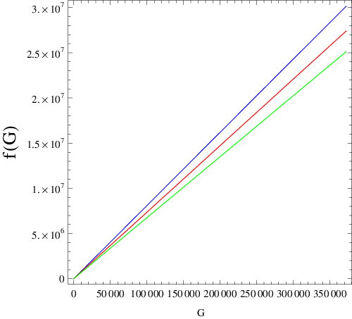
The reconstructed presented in Eq. (12) is plotted against in Fig. 1, where we have taken and . The red, green and blue lines correspond to and respectively. It is observed in the figure that as . This indicates that the reconstructed represents a realistic model.
Using Eqs. (12), (13) and (14) in (3) we get reconstructed as
| (15) |
In Eq. (15) it is essential that . Similarly, using Eqs. (12), (13) and (14) in (4) we get reconstructed as
| (16) |
In Eq. (16), . Conservation equation for pressureless () dark matter is
| (17) |
that gives
| (18) |
Using Eqs. (15), (16) and (18) the effective EoS parameter is found to be
| (19) |

The EoS parameter presented in Eq. (19) is plotted in Fig. 2, where we have taken and . We have presented in a 3D plot for a range of values on over redshift . It is observed that for smaller values of , over the entire range of . However, for larger values of e.g. , with evolution of the universe i.e. reaches phantom boundary, but never crosses it. Currently, i.e. for , . Thus, in general, the behaves like quintessence (Cai et al., 2010).
III GSL in QCD ghost gravity
Since the discovery of black hole thermodynamics in 1970s, it has been speculated by physicists that there should be some relationship between thermodynamics and Einstein equations because the horizon area (geometric quantity) of black hole is associated with its entropy (thermodynamical quantity), the surface gravity (geometric quantity) is related with its temperature (thermodynamical quantity) in black hole thermodynamics (Akbar and Cai, 2006; Jamil et al., 2012). In analogy with black hole thermodynamics, investigating thermodynamics laws for cosmological horizons, which are present in many of cosmological models, has also been the subject of many studies (e.g. Busso, 2005; Jamil et al., 2010 (a, b); Sadjadi, 2011; Saridakis et al., 2009; Debnath et al., 2012; Jamil et al., 2012a). Here we mention some examples of exploration of the generalized second law (GSL) of thermodynamics in modified gravity scenario. Bamba and Geng (2009) demonstrated that an gravity model with realizing a crossing of the phantom divide can satisfy the GSL in the effective phantom phase as well as non-phantom one. Bamba and Geng (2011) explored thermodynamics of the apparent horizon in gravity with both equilibrium and non-equilibrium descriptions. Karami and Abdolmaleki (2012) investigated the validity of the generalized second law (GSL) of gravitational thermodynamics in the framework of modified teleparallel gravity. Chattopadhyay and Ghosh (2012) established validity of GSL in the modified f(R) Horava–Lifshitz gravity.
Here, we investigate the validity of the GSL for a spatially flat FRW universe. Hawking temperature on the apparent horizon is given by
| (20) |
where ensures .
The entropy of the universe including the dark matter inside the dynamical apparent horizon is given by Gibb’s equation
| (21) |
where, and is the volume containing the pressureless dust matter with the radius of the dynamical apparent horizon . Also,
| (22) |
From the modified field equation if we write then we can have
| (23) |
In the thermodynamics of the apparent horizon in the Einstein gravity, the geometric entropy is assumed to be proportional to its horizon area . However, this definition is changed for other modified gravity theories. The geometric entropy in gravity is given by , where . In gravity, it was shown that when is small, the first law of black hole thermodynamics is satisfied approximatively and the entropy of horizon is , where . In the present case, where we are considering gravity, we compute
| (24) |
From (24) it is easy to get
| (25) |
| (26) |

The time derivative of total entropy derived in Eq. (26) for the QCD ghost gravity given by Eq. (12) is presented in Fig. 3 for a range of against redshift and it is observed that for the entire range of we have and this indicates validity of GSL for this QCD ghost gravity with apparent horizon as the enveloping horizon of the universe. It is also observed that is decreasing with for a given redshift and is increasing with evolution of the universe.
IV Concluding remarks
In the present study we have presented a reconstruction scheme for gravity, where represents Gauss-Bonnet invariant and we have chosen the scale factor in power-law form. Considering a flat FRW universe, we have considered a correspondence between gravity and QCD ghost dark energy. After getting a reconstructed solution for in Eq, (12) we have plotted against , where it is apparent that as , which is one of the sufficient conditions for a realistic model. In Eq. (19) we have plotted the effective equation of state parameter for in Fig. 2 and observed that i.e. it behaves like quintessence. For , is reaching at late stage of the universe. However, it is not crossing the phantom boundary. Subsequently, considering dynamical apparent horizon as the enveloping horizon of the universe we have derived expression for the time derivative of total entropy in Eq. (26) and we have observed that throughout the evolution of the universe. This indicated validity of the generalized second law of thermodynamics under this reconstruction of gravity.
IV.1 Acknowledgement
Financial support from Department of Science and Technology, Govt. of India, under Project Grant No. SR/FTP/PS-167/2011 is duly acknowledged.
References
Akbar, A., Cai, R. G.: Phys. Lett. B 635, 7 (2006)
Abazajian, K., et al.: Astron. J. 128, 502 (2004)
Abazajian, K., et al.: Astron. J. 129, 1755 (2005)
Allen, S.W., Schmidt, R.W., Ebeling, H., Fabian, A.C., van Speybroeck,
L.: Mon. Not. R. Astron. Soc. 353, 457 (2004)
Bamba, K., Capozziello, S., Nojiri, S., Odintsov, S. D.: Astrophys. Space Sci. 341, 155 (2012)
Bamba, K., Geng, C-Q.: JCAP 11, 008 (2011) doi:10.1088/1475-7516/2011/11/008
Bamba, K., Geng, C-Q.: Phys. Lett. B 679, 282 (2009)
Bennett, C.L., et al.: Astrophys. J. 583, 1 (2003)
Bousso, R.: Phys. Rev. D 71, 064024 (2005)
Cai, Y. F., Saridakis, E. N., Setare, M. R., Xia, J. Q.: Physics Reports, 493, 1 (2010)
Copeland, E.J., Sami, M., Tsujikawa. S.: Int. J. Mod. Phys. D 15, 1753 (2006)
Chattopadhyay, S., Pasqua, A.: Astrophys. Space Sci. 344, 269 (2013)
Chattopadhyay, S., Ghosh, R.: Astrophys. Space Sci. 341, 669 (2012)
Clifton, T., Ferreira, P.G., Padilla, A., Skordis, C.: Phys. Rep. 513, 1
(2012)
Debnath, U., Chattopadhyay, S., Hussain, I., Jamil, M., Myrzakulov, R.: Eur. Phys. J. C 72, 1 (2012) 10.1140/epjc/s10052-012-1875-7
Garcia-Salcedo, R., Gonzalez, T., Quiros, I., Thompson-Montero, M.: Phys. Rev. D 88, 043008 (2013)
Houndjo, M. J. S., Rodrigues, M. E., Momeni, D., Myrzakulov, R. arXiv preprint arXiv:1301.4642 (2013)
Jamil, M., Momeni, D., Myrzakulov, R.: Eur. Phys. J. C 72, 2137 (2012)[arXiv:1210.0001 [physics.gen-ph]]
Jamil, M., Yesmakhanova, K., Momeni, D., Myrzakulov, R.: Central Eur. J. Phys. 10, 1065 (2012)
[arXiv:1207.2735 [gr-qc]].
Jamil, M., Saridakis, E. N., Setare, M. R.: Phys. Rev. D 81, 023007 (2010a)
Jamil, M., Saridakis, E. N., Setare, M. R.: JCAP 11, 032 (2010b) doi:10.1088/1475-7516/2010/11/032
Jamil, M., Momeni, D., Myrzakulov, R. Chinese Physics Letters 29, 109801 (2012)
Jawad, A., Pasqua, A., Chattopadhyay, S.: Astrophys. Space Sci. 344, 489 (2013)
Jamil, M., Momeni, D., Raza, M., Myrzakulov, R.: Eur. Phys. J. C 72, 1 (2012a)
Jamil, M., Momeni, D., Bamba, K., Myrzakulov, R. : Int. J. Mod. Phys. D 21, 1250065 (2012) DOI: 10.1142/S0218271812500654
Li, M., et al.: Commun. Theor. Phys. 56, 525 (2011)
Myrzakulov, R., Sáez-Gómez, D., Tureanu, A.: Gen. Relativ. Gravit.
43, 1671 (2011)
Nesseris, S., Basilakos, S., Saridakis, E. N., Perivolaropoulos, L.: Phys. Rev. D 88, 103010 (2013)
Nojiri, S., Odintsov, S.D.: Int. J. Geom. Methods Mod. Phys. 4, 115
(2007)
Nojiri, S., Odintsov, S.D.: Phys. Lett. B 631, 1 (2005)
Ohta, N.: Phys. Lett. B, 695, 41 (2011)
Padmanabhan, T.: Curr. Sci. 88, 1057 (2005)
Perlmutter, S., et al.: Astrophys. J. 517, 565 (1999)
Rodrigues, M. E. , Houndjo, M. J. S. ,Momeni, D., Myrzakulov, R.: Can. J. Phys. 92, 173 (2014)
Sadjadi, H. M., Phys. Scr. 83, 055006 (2011)
Saridakis, E. N., Gonzalez-Diaz, P. F., Sigüenza, C. L.: Class. Quantum Grav. 26, 165003 (2009) doi:10.1088/0264-9381/26/16/165003
Setare, M.R.: Phys. Lett. B 644, 99 (2007a)
Setare, M.R.: Phys. Lett. B 648, 329 (2007b)
Setare, M.R.: Phys. Lett. B 653, 116 (2007c)
Setare, M.R. and Saridakis, E. N.: Phys. Lett. B 670, 1 (2008)
Spergel, D.N., et al.: Astrophys. J. Suppl. Ser. 148, 175 (2003)
’t Hooft, G.: arXiv:gr-qc/9310026 (1993)
Tegmark, M., et al.: Phys. Rev. D 69, 103501 (2004)
Urban, F. R., Zhitnitsky, A. R.: Nucl. Phys. B, 835, 135 (2010a)
Urban, F. R., Zhitnitsky, A. R.: Phys. Lett. B, 688, 9 (2010b)