Biased random walks on random graphs
Key words and phrases:
random walk in random environment, Galton-Watson tree, percolation clusters, I.I.C., stable laws, subordinators, aging, traps, extremal process, infinitely divisible distributions, electrical networks2000 Mathematics Subject Classification
primary 60K37, 60F05, 60J80; secondary 60E071. Introduction
These notes cover one of the topics programmed for the St Petersburg School in Probability and Statistical Physics of June 2012. The aim is to review recent mathematical developments in the field of random walks in random environment (RWRE). For a detailed background on RWREs we refer the reader to [81] or [78].
Our main focus will be on directionally transient and reversible random walks on different types of underlying graph structures, such as , trees and for .
Rather than speaking abstractly about the current state of the field, we decide to first dive into the heart of the subject by presenting rapidly a simple model which encapsulates most of the key questions we want to address in those notes. We feel this will give the reader a clear framework and provide an early motivation to understand the issues at hand.
1.1. The key issues in one simulation
We introduce informally the model of the biased random walk on a Galton-Watson tree with leaves (a more detailed description of this model can be found in Section 3).
Given a tree and , we can define the -biased random walk on the tree . It is a Markov chain on the vertices of , such that if and has children and parent , then
- (1)
,
- (2)
, for ,
and from the root all transitions to its children are equally likely. The walk is typically started at the root.

The biased random walk on a Galton-Watson tree with leaves is obtained by choosing to be a supercritical Galton-Watson tree with leaves (i.e. positive probability of having no offspring) conditioned to be infinite. We use the probability to have offspring for the unconditioned Galton-Watson tree (in particular, our assumptions is that ).
We recall some of the most basic facts known about this walk (we will give details on this in Section 3). Firstly, there exists a constant such that
by results in [57] and where denotes the usual distance on trees. Secondly, for , we have that (see [60])
where the limiting speed depends not only on but also on the offspring distribution. We choose to omit this dependence during the introduction.
The first result means that the walk is transient and the second means it has an asymptotic velocity depending on the law of the tree and the bias. Both results hold almost surely in the environment and the walk.
An interesting picture arises when one looks at simulations of the velocity (also called speed) as a function of the bias for three different choices of trees, see Figure 2, 3, 4. In these simulations, the speed is estimated after 10 million steps.
Remark 1.1.
It is important to emphasize that the speed is very hard to estimate through simulations for “large” values of the bias. Indeed, because of the trapping naturally occurring in this model, the convergence of towards the limiting velocity is very slow. The speed obtained through simulations is generally noticeably superior to the true speed for large values of the bias.
Nevertheless the simulations highlight several interesting features of this model and provide a very visual motivation for studying this model so we decided to include them. A qualitative representation of what the asymptotic speed should look like will be given later in these notes (see Figure 13).


From these simulations, we seem to detect some similar patterns
- (1)
the speed first increases and then decreases (this is called unimodality),
- (2)
the speed is eventually zero.
At any point of the tree an increase in the bias will increase the local drift away from the root (only at leaves does the drift remain unchanged). Yet, the walk is not necessarily sped up, actually, for stronger biases the motion eventually has zero speed.
The reason for the sub-ballistic regime is that the walk loses time in ‘traps’ within the tree, from where it cannot go to infinity without having to battle for a long time against the drift which pushes it into the trap. The hypothesis is crucial for this to happen, since it is the leaves that create those dead-ends (see Figure 1). The case illustrates this phenomenon to the extreme since it turns the walk recurrent.
From these observations a set of very natural question appears,
- (1)
Is it true that the speed is unimodal?
- (2)
Is it true that the speed is eventually zero?
- (3)
How fast does the walker move when its speed is zero? After proper rescaling, what are the scaling limits of distance of the random walk from the origin?
1.2. Goal of the notes
The example we chose is convenient because it is simple to define mathematically and yet raises interesting questions. Nevertheless, the reader might question its relevance. As it turns out this model was considered as an approach to the more difficult problem of biased random walks on percolation clusters (a model presented in Section 4.1). This model already attracted the attention of physicists in the 80s, see [5], [28] and [29], not only for its interesting phenomenology but also because it presents similarities to concrete physical systems such as diffusion of particles in gels under gravity, or in centrifugal forces as in chromatographic columns, and hopping electron conduction in doped semiconductors in the presence of strong electric field. For a physical perspective on biased diffusion in disordered media, we invite the reader to take a look at Chapter 6 of the overview [47].
From a more mathematical perspective, biased random walks on percolation clusters have also received a lot of attention. This has been part of the larger project of trying to understand RWREs on (for ), subject that has been very active in the last decade, following namely an important work of Sznitman and Zerner, see [79]. Although the field of RWREs is very wide, see [81] or [78] for overviews, we will chose to ignore a large part of it and focus on the case of reversible and directionally transient RWREs.
These types of models have long been known to be related to trapping. But it is only in the last few years that concrete links have been established between RWREs (that are directionally transient and reversible) and dynamics of traps models, more specifically a directed version of the so-called Bouchaud Trap Model (BTM) (introduced in [20]). This model, originally introduced to understand dynamics of spin glasses, turned out to be a key tool in understanding RWREs.
Our main goal is not to give a thorough overview of trap models, a topic covered in details in [11]. Rather, one of our goals will be to explain how a variety of models: biased random walks on Galton-Watson trees, on percolation clusters and many RWREs on can all be linked to one single trap model. This link is the crucial element to prove of a myriad of interesting properties such as anomalous scaling limits and aging for a wide class of RWREs. This will provide a very complete answer to the last two questions asked at the end of the previous section.
Another goal will be to study trapping under a different light for which RWREs offer a natural setting: understanding the influence of traps on the limiting velocity of random dynamics. In our concrete example of biased random walks on Galton-Watson tree with leaves, we can effectively tune the strength of the trapping by changing the value of , and, as we saw in Figure 2-3-4, this can be felt in the behavior of the limiting velocity in function of . The exact nature of this link is an interesting subject where deceivingly simple questions remain open.
1.3. Plan of the notes
We will take a progressive approach where we start from easier models and build up to more sophisticated examples. We start in Section 2 by presenting models where the underlying graph is one-dimensional, this will include a key toy model (called the directed Bouchaud Trap Model) and one-dimensional random walks in random environments. This first part is somewhat at odds with the rest of these notes that will focus on RWREs on trees and . Nevertheless, it allows for a simple way to showcase the parallel between trap models and RWREs.
The second main section (Section 3) of this paper will be devoted to RWREs on Galton-Watson trees, our main objective being to study the properties of the limiting velocity and the scaling of such process. Our main focus will be on biased random walks in a wide variety of settings: on Galton-Watson trees with leaves, without leaves and we will also discuss the case of randomly chosen biases.
Then, in Section 4, we move on to the biased random walks on percolation clusters and present the latest results concerning the long term behavior of such walks (speed, scaling limits …),
Finally, we shall give an overview of related results on critical structures, namely the infinite incipient cluster (or I.I.C.) on trees or the lattice, in Section 5.
Most of the work presented in these notes was developed in the last five years, hence many questions remain open. We will include at the end of most sections a list of open problems related to the material presented in the corresponding section.
At the end of the paper, we include a brief appendix covering some basic facts on sums of heavy-tailed i.i.d. random variables, a key element for understanding trapping in directionally transient RWREs.
2. One dimensional models
Our first goal in this notes is to introduce the key toy model for understanding RWREs in the directionally transient regime. We will show how this elementary model is representative of more complex models, namely one-dimensional RWREs.
2.1. The totally directed Bouchaud Trap Model
We introduce a sequence of positive i.i.d. random variables. In the context of trap models, these random variables constitute our environment and represent the strength of the different traps. They are usually assumed to have heavy tails but for the time being we will not make any further assumptions.
The totally directed Bouchaud Trap Model is a nearest-neighbor continuous-time Markov process with state space . Its dynamics are very simple, spends at a site an exponentially distributed time of mean (we recall that was chosen randomly) and then jumps to its right neighbor. Our goal is to see how fast moves.
The analysis of this model is pretty elementary. Its interest comes from the fact that several types of biased (or directionally transient) RWREs can be compared to this toy model as will become apparent through these notes.
One key random variable to understand how fast moves is the time it takes us to make steps (and thus reach ). This quantity can be written
| (2.1) |
where is a family of i.i.d. mean-one exponentially distributed random variables.
It is simple to notice that
| (2.2) |
where the right-continuous inverse of an increasing function is defined by . This equation will allow us to derive scaling limits of from those of by elementary inversion arguments.
The reason why it is convenient to consider is that it is simply a sum of i.i.d. random variables. The topic of sums of i.i.d. random variables is very well understood and thus it is possible to give a complete picture of all the possible behaviors for scaling limits of . Since a lot of the results in these notes boil down to sums of i.i.d. random variables, it is very important for the reader to be familiar with the subject. We refer the reader to the Appendix for a brief overview of certain key facts related to sums of i.i.d. heavy-tailed random variables.
The most trivial case is when in which case we have the law of large numbers and a central limit theorem for . Denoting (for velocity), we have
which, by a standard inversion argument, translates into
One could also easily prove that the processes
and
both converge as goes to infinity to Brownian motions in the Skorohod topology, see Chapter 3 of [38].
In cases where , we start feeling the effects of traps and witnessing anomalous (non-Gaussian limiting behavior) and we will from now on solely focus on this case.
To simplify the notations we will assume that for . Although this might seem like an arbitrary choice, up to a scaling by a constant, this covers all tails of the form . Most cases appearing in models of biased RWREs fall into that category and, thus, the results in next sections are the ones we expect to witness for many biased RWREs where trapping occurs.
Remark 2.1.
Up to some minor changes in the centering and the scaling in the coming results, all of them can be carried over to the case where where and is a slowly varying function (see the Appendix, definition 6.4, for a precise definition).
2.1.1. The case
In this section, we assume for . In this case, the trapping is very strong and we actually have , this means that even the law of large numbers fails for . Let us state what kind of results can be obtained in this case.
Stable laws as scaling limits
First, we see that has zero-speed and should be rescaled as . The proper rescaling leads to stable scaling limits:
| (2.3) |
where is a completely asymmetric positive stable random variable of index (see the Appendix, Section 6.1.1 for a more precise definition).
Stable subordinators as limiting processes
These results carry over to the process level. Indeed, if we consider, for fixed, the processes
| (2.4) |
and
then the law of defined on the space of càdlàg functions from to equipped with the Skorohod -topology (see [80] for a detailed account on this topology) converges weakly to the distribution of
| (2.5) |
where is an -stable subordinator (see the Appendix, Section 6.2.1, for a precise definition). Moreover, the law of of defined on equipped with the uniform topology converges weakly to the law of
| (2.6) |
where is the inverse of an -stable subordinator.
Aging properties
Aging is one of the main paradigms in dynamics in random media. It appears in the context of dynamics on spin glasses [7] (see [20] for a physical overview of spin glasses) as well as in the random energy model under Glauber dynamics [8]) or in parabolic Anderson model (see [66]). A dynamic satisfies aging if the right time scale to witness a significant change in the system is of the order of the ‘age’ of the system (i.e. the time during which the dynamics has run).
In our context, this can be expressed in the following property: for all with , we have
| (2.7) |
where the integral on the right side can be rewritten as , where denotes the generalized arcsine distribution with parameter . The arcsine law is a distribution on .
2.1.2. The case
In this section we assume for . In this case we still have , and thus the law of large numbers holds
where .
The trapping is actually felt in the fluctuations of the walk.
Stable laws in the fluctuations
where is a completely asymmetric zero-mean stable random variable of index (see the Appendix, Section 6.1.1 for a more precise definition).
Stable totally asymmetric Lévy processes as limiting processes for the fluctuations
For fixed, if we define the processes
and
then the law of defined on the space of càdlàg functions from to equipped with the Skorohod -topology converges weakly to the distribution of
where is an -stable totally asymmetric Lévy process (see the Appendix, Section 6.2.1, for a precise definition). Moreover, the law of defined on equipped with the uniform topology converges weakly to the law of
where is an -stable asymmetric Lévy process (with the same law as the one appearing in the previous equation).
2.2. The biased Bouchaud Trap Model
Let us define the biased Bouchaud Trap Model. Again we choose a sequence of positive i.i.d. random variables, and assume that
for some .
For any , the -biased Bouchaud trap model is defined in the following manner: started at , the walk spends at any site an exponentially distributed time of mean and then jumps to the right with probability and to the left with probability .
Remark 2.3.
The totally directed Bouchaud trap model is the particular case .
We choose to view as a time change of a discrete biased random walk on . For this, we denote by
- (1)
a -biased random walk on recording the successive locations of
- (2)
the time of the -th jump of which can be written where is a family of i.i.d. mean-one exponentially distributed random variables.
In this context, and are respectively called the embedded process and the clock process.
We emphasize that we changed our definition of compared to the previous section (we replaced by ), although in the case these definitions coincide since . It is then simple to notice that
where the right-continuous inverse of an increasing function is defined by .
Remark 2.4.
One of the purposes of this transformation is to notice the link with biased random walks in random environment. The bias is encoded in the embedded process and the random environment is felt in the clock process.
The key difficulty is the interplay between the past trajectory and the clock process, in particular is no longer a sum of i.i.d. random variables. In this context, the time spent in a given trap is determined by two elements: the number of visits to that trap and the time spent during each of those visits. Although for two distinct traps the time spent during visits in those traps is still independent the number of visits to two adjacent traps is very much correlated. One could then be led to believe that the results obtained through classical theorems on sums of i.i.d. random variables will fail.
Nevertheless, it turns out that the following result is true, see [82].
Theorem 2.1.
Let us consider trapping times which are positive i.i.d. random variables such that , for some . Then the -directed Bouchaud trap model has stable limit laws, stable subordinators as limiting processes and verifies the aging property.
More precisely, the properties listed at (2.3), (2.4), (2.5) and (2.6) remain true in the case of the -directed Bouchaud trap model. The only difference is that the limiting -stable laws (or subordinators) have different parameters (see the Appendix, Section 6.2.1, for precise definitions). Furthermore, the property (2.7) is conserved exactly as it is.
This result raises a natural question: why does the model not feel the dependencies?
Remark 2.5.
Similar results to Section 2.1.2, should be true for this model when .
2.2.1. Why do trap models ignore many dependencies?
Let us consider trapping times which are positive i.i.d. random variables such that
for some .
Our goal is to intuitively explain why a directed trap model with such trapping times is insensitive to many correlations: why is it that (defined after Remark (2.3)) still behaves as a sum of i.i.d. random variables?
To compute the hitting time , the interval is essentially the only one relevant for us. Indeed the directed nature of the walk makes us unlikely to visit many sites at the left of the origin (at most ). An elementary computation shows that the deepest traps (i.e. those of maximal mean waiting time) encountered in the interval is of the order . Fix , the previous brings us to the following observations.
- •
Before , we are only visiting traps of depth (i.e. mean waiting time) less than .
Also, we can actually estimate the number of deep traps encountered.
- •
Before , we visit roughly traps of depth larger than . They are also spatially very well separated (at typical distance ). Since the walk is unlikely to backtrack (go towards the left) for more than steps, the behavior of the walk (number of visits …) in two different large traps is essentially independent.
Finally, small traps are irrelevant as far as limiting behaviors are concerned.
- •
Before , the total time spent in all traps of depth less than is .
Hence
where the are i.i.d. and represent the total time spent in traps conditioned to be larger than . This setting is not the standard one of sums of i.i.d. random variables. Indeed, the law of the terms is -dependent. Nevertheless this object is known as a triangular array and the limiting behavior of triangle arrays is very well understood (see [70]). It is by using limiting theorems on such triangular arrays that we can manage to obtain stable scaling limits.
2.3. The one dimensional random walk in random environment
Up to this point we have only considered toy models, in which traps were introduced ad hoc, by forcing waiting times at different sites. This allowed us to understand which limiting results we can expect when trapping is involved and at the same time it gave us an opportunity to describe the way trap models work.
We will present a random dynamic in random media which does not have the trapping encoded in its definition but yet exhibits the same type of limiting behaviors: one dimensional random walks in random environments.
One-dimensional random walks in random environment to the nearest neighbors were introduced in the sixties in order to give a model of DNA replication. Mathematically, these models were initially studied in the seventies and are still yielding new results up to the present day.
2.3.1. The model
Let be a family of i.i.d. random variables taking values in defined on which stands for the random environment. Denote by the distribution of and by the corresponding expectation. Conditioning on (i.e. choosing an environment), we define the random walk in random environment as a nearest-neighbor random walk on with transition probabilities given by : is the Markov chain satisfying and for

We denote by the law of and the corresponding expectation. It is usually called quenched law. Also we denote by the joint law of , which is referred to as averaged or annealed law.
2.3.2. The results
In the study of one-dimensional random walks in random environment, an important role is played by the sequence of variables
since their law will allow to see when the walk is transient, recurrent, has positive speed, or not.
We assume that is well defined (possibly infinite). Then we obtain a criterion for transience and recurrence, see [74].
Theorem 2.2.
- (1)
If (respectively ¿0) then the walk is transient and
- (2)
If , then the walk is recurrent and
An explanation for the result of this theorem is given at the beginning of Section 2.3.3.
Our goal being to focus on the transient case, so we shall henceforth assume that (which is possible by symmetry). If the reader wants more information on the recurrent case, he/she should consult [73]. Since we assume directional transience to we can introduce, for ,
| (2.8) |
the hitting time of .
We may decide whether the walk has positive speed or zero velocity, see [74].
Theorem 2.3 (Solomon-1975).
If we have , then
with
The key fact here is that it is possible to obtain directional transience towards and yet have zero speed which is indicative of trapping. This means we should be expecting stable laws in the limit, and indeed
Theorem 2.4.
Let us assume that
- (1)
,
- (2)
there is a such that and
- (3)
the distribution of is non-lattice (that is, the -linear span of is dense in ),
then
- •
if , letting , we have
- •
if , then
where is a completely asymmetric stable law of index .
A more complete result, covering the case and , can be found in [54]. The original proof of Kesten, Kozlov and Spitzer gives a very complete result using a short proof related to branching processes. Although efficient this argument is very specific to and could not be carried over to different underlying graphs.
An alternate proof of the previous result was obtained in [33] and [34] (for ) and later completed in [37] (for ). This alternate proof used the similarities of one-dimensional RWREs and the biased Bouchaud trap model. To the best of our knowledge, it was the first successful attempt to link directly RWREs to trap models. The works [33] and [34] actually predate and inspired the work on biased trap models [82] that we presented earlier.
Remark 2.6.
Remark 2.7.
A key benefit of this trap model approach is that it allows one to obtain the following aging result when , which was previously unknown, see [35].
Theorem 2.5 (Enriquez, Sabot, Zindy - 2009).
Let us assume that
- (1)
,
- (2)
there is a such that and
- (3)
the distribution of is non-lattice,
then, for any and any , we have
An other, even more important, consequence of this work is that it provided methods that could later be used to analyze RWREs on different graphs such as trees and ().
2.3.3. Parallel between one dimensional RWREs and the biased BTM
The parallel one dimensional RWREs and the biased BTM can be made by considering an object called the potential that was introduce in 1982 by Sinai [73].
| (2.9) |
This potential gives a nice intuitive vision of the transition probabilities. Loosely speaking it could be seen as an altitude profile on which the walker will move, favoring directions going downhill. Mathematically, we see that
- •
is a random walk with i.i.d. steps of law . This means it can be analyzed very precisely.
- •
is linked to an invariant measure of the walk in the environment by setting . This explains why the walk is attracted to parts where is small.

Let us detail the strategy used in [33] and [34] to link one-dimensional RWREs to the biased BTM using the potential . In Figure 6, we have singled out parts of the environment where the walk needs to walk uphill against the potential to reach . These valleys create obstacles that prevent the walk from going easily to . These obstacles have a random height which can be shown to verify
| (2.10) |
When in a valley of height , the walk will need a certain time to exit it. To simplify the argument, we use the approximation where is an exponential random variable of parameter 1. A reader interested in deeper details on this issue might want to look at Section 3.3.4 and Remark 3.21 for a deeper discussion on a similar problem in a different context. Using the tail estimate on we obtain
which is the heavy-tailed random variable we were expecting to see when .
The parallel with the biased BTM should now be pretty clear. A few issues might still bother the reader:
- (1)
The embedded walk is no longer a biased random walk. While this is true, we only really need for the embedded walk to go against the direction of transience for small distances (at most before time , see (2.8) for the definition). This is still verified in the model.
- (2)
The trap depth are no longer independent, indeed many neighboring sites are in the same valley and share similar exit times. This issue can be resolved by considering the entire valleys as one trap (or a site in the biased BTM) since valleys are typically small (at most before time ) they appear as points when rescaled in an environment of length . One can then argue that the heights and geometry of the largest traps is roughly independent since they are located far from each other.
3. Biased random walk on supercritical trees
3.1. The model
The model of biased random walk on supercritical Galton-Watson trees was initially studied in [60]. As discussed in the introduction, it has an interesting phenomenology and is a natural setting for discussing trapping issues.
3.1.1. Definition
Consider a supercritical Galton-Watson branching process with generating function , i.e. the offspring of all individuals are i.i.d. copies of , where . We assume that the tree is supercritical, i.e. . If , the tree has no leaves and otherwise it does. We denote by the extinction probability ( since the tree is supercritical), which is characterized by . We know that if, and only if, . Starting from a single progenitor called root and denoted by , this process yields a random tree . If , we will always condition on the event of non-extinction, so that is an infinite random tree. We denote by the associated probability space: is the law of the original tree, conditioned on non-extinction.
Given such an infinite Galton-Watson tree , we consider the -biased random walk started at as defined in Section 1.1. For a fixed environment , the associated law of the -biased random walk is called quenched and is denoted . We define the averaged (sometimes called annealed) law as the semi-direct product .
Remark 3.1.
For a vertex , we denote by the distance of to the root.
3.1.2. Basic results
Expanding on the results of Section 1.1, we have, by [57], the following recurrence and transience criterion.
Theorem 3.1.
Let be a -biased random walk on a Galton-Watson tree with law . We have the following
- •
if , then is strongly recurrent -a.s. for -almost all .
- •
if , then is null recurrent -a.s. for -almost all
- •
if , then is transient -a.s. for -almost all which means that ,
In the sequel we will, unless stated otherwise, assume that which means that we have transience of towards .
The next natural question, that of the behavior of the speed, was investigated in [60].
Theorem 3.2.
We have
Furthermore
- (1)
if , then ,
- (2)
if , then if and if where .
Remark 3.2.
We emphasize that (see Remark 3.3). This means that the zero-speed regime only occurs if , that is if the walk is outwardly-biased.
This means that we can answer the second question asked at the end of the introduction (just before Section 1.2) affirmatively: the speed has a sharp phase transition from positive speed to zero speed.
As previously mentioned this result is due to the existence of dead ends in the tree creating trapping structure for a strongly biased walk, see Figure 1. In the next section, we will introduce the Harris-decomposition for Galton-Watson trees. This construction allows us to describe precisely the structure of traps. It is key to understand the link between biased random walks on Galton-Watson trees and traps models. This subject will be treated in more details in Section 3.3.1.
3.1.3. The Harris-decomposition of Galton-Watson trees
Set
| (3.1) |

Remark 3.3.
The functions and have a nice graphical representation, see Figure 7. Here, we can easily see that .
It is known (see [57]), that a -Galton-Watson tree (with ) can be generated by
- (1)
growing a -Galton-Watson tree called the backbone, where all vertices have an infinite line of descent,
- (2)
attaching on each vertex of a random number of subcritical (hence finite) -Galton-Watson trees, acting as traps for the biased random walk,
where has a distribution depending only on and given and the traps are i.i.d. (see [57] for details).

The Harris-decomposition, see Figure 8, allows us to view the biased random walk on the Galton-Watson tree with leaves in terms very similar to those of the trap models introduced so far. Indeed, one may view the walk on the backbone as the embedded process on a leafless -Galton-Watson tree with waiting times in traps given by excursion times in -Galton-Watson trees (recall Section 2.2 for the vocabulary associated to trap models).
3.2. The asymptotic speed
Let us turn to the first question at the end of the introduction (just before Section 1.2), and try to see if, in the case with leaves, it is true that the speed is unimodal, meaning it is first increasing and then decreasing.
At first sight, the embedded process and the waiting times are in competition to determine the value of the velocity.
- (1)
On the backbone, there are no hard traps for the walk. This would lead one to believe that increasing the bias would increase the speed of the embedded process.
- (2)
On the other hand, increasing the bias increases the time spent in traps and so delays the walk.
The second point can be shown to be true, at least in expectation, using the mean return time formula (a particular case of the commute time formula, see [21]). The first point, however, is not as simple of a question as it may seem. It leads us to the following question which was asked in 1996 (see [60] and [62]).
Question 3.1.
Is the speed of a biased random walk on a Galton-Watson tree without leaves increasing (or even non-decreasing) ?
3.2.1. The asymptotic speed on trees without leaves
At first sight it seems that the speed of a biased random walk (as defined in the introduction) on any leafless tree should be non-decreasing. Nevertheless this is wrong as some examples from [62] show. This section is devoted to presenting some of the examples of [62] and their behavior.
Example 1: Binary tree with pipes
Let be a binary tree to which we add a unary tree, which we refer to as a pipe, at every vertex, see Figure 9.
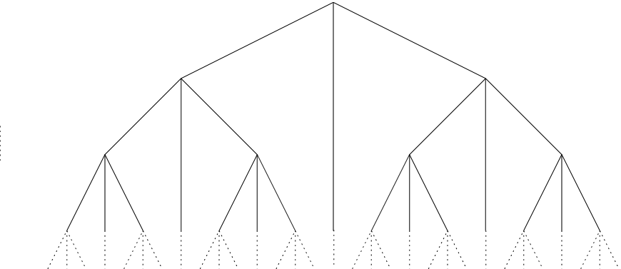
It is elementary to see that the walk becomes transient for . We can then observe the following.
- (1)
For , the walk has barely turned transient and its speed should be small: .
- (2)
For , we are looking at the simple random walk which is known to have a (finite) return time with infinite expectation in each pipe. The walk can only go to infinity through the binary part of the tree. However, on its way it will regularly enter pipes and lose a substantial amount of time in them (each excursion having infinite mean). This will mean that .
- (3)
For , the walk on the binary part has speed (by comparing it to a -biased random walk on ) and the excursions on the pipes will be brief. This means that is bounded away from .
For more details on this, we refer the reader to Example 2.1 in [62].
Even though this example clearly shows a mechanism for slowing down the walk whilst increasing the bias, it is slightly dissatisfying. Indeed the cause for the slowdown observed in the second point is that pipes act, de facto, as traps. This makes this example somewhat artificial. In order to prevent such examples, one could impose for the bias to be larger than . This would prevent us from creating hard traps without using leaves.
Remark 3.4.
We emphasize that in the previous example the speed coincides with that of a -biased random walk on for .
Example 2: The filtering method
We shall explain how to proceed to create a tree on which the -biased random walk has a higher speed than the -biased random walk for .
The key fact we use is the following: there exists a tree such that given there exists sufficiently large and two complementary subsets and of the -th level of such that the first visit of the -biased random walk to level on first reaches with probability at least .
This property is verified by almost every tree produced from a Galton-Watson process with mean larger than . We take this fact as a given for our upcoming construction. This property of Galton-Watson trees follows from the fact that on such a tree the harmonic measure of the -biased random walk are singular, a fact proved in Lemma 5.2 of [60]. The reader may find more details on this in [60] or [59].
Then we apply the following procedure: keep the first levels of , add (with ) levels of a -ary tree to each vertex of and we call the resulting tree . We choose large enough to ensure that the -biased random walks are unlikely to revisit the root of a -ary tree. Also we choose , so that the -biased random walk on the -ary tree is faster than the -biased random walk on a -ary tree.

The dynamics on this tree, see Figure 10, are as follows
- (1)
the -biased random walk will, w.h.p., be in when it reaches the -th level of ,
- (2)
from there, the walk will move for a long time on a -ary tree, hence, its overall speed will progressively become close to that of the -biased random walk on a -tree.
Essentially, the time spent in the first section of the tree can be made small in comparison to the time spent in the second section, so the total speed is determined mainly by the second part of the journey. In particular the -biased random walk is faster than the -biased random walk on .
To finish the argument, we take , add to each of its leaves a copy of and repeat the procedure constructing an infinite tree . It is clear that on , increasing the bias from to will slow the walk down.
Remark 3.5.
The construction of the filtering part of the tree which separates walks of different bias ( in the previous example) can also be done in a deterministic manner. Hubert Lacoin has exhibited explicit examples on which the speed can be computed exactly and, indeed, turns out not to be increasing. (Personal communication from Hubert Lacoin).
Of course none of these trees are Galton-Watson trees (although they are multi-type Galton-Watson trees) so we do not have any counter-examples to Question 3.1. We merely wanted the reader to appreciate the complexity of the question.
3.2.2. The asymptotic speed on Galton-Watson trees without leaves
Recently, some progress has been made in understanding the speed of biased random walks on Galton-Watson trees without leaves. We shall review the main results.
Theorem 3.3.
The speed of a -biased random walk on a Galton-Watson tree without leaves is increasing for .
Furthermore, for a -biased random walk on a Galton-Watson tree with minimal degree , the speed of this biased random walk is increasing for .
Remark 3.6.
The threshold 1160 is completely arbitrary and could be lowered using the methods of the paper. Nevertheless, the threshold cannot be lowered to any value that would have any particular significance such as or .
The proof relies on a coupling of three distinct walks: two biased walks ( and ) on Galton-Watson trees and a -biased random walk on . Once this coupling is in place the proof turns out to be surprisingly elementary.
In some very vague sense, the high bias ensures that the biased walks interact very little with their environment. With the environment out of the picture, the decisive element for a faster speed is the bias. The third walk in the coupling provides an upper bound on the interaction of the walks with the environment.
Remark 3.7.
The techniques in the proof of Theorem 3.3 are somewhat robust. This would lead us to believe that they could be adapted to different problems. In particular, we would think that it should be possible to use these methods to prove that the speed of a -biased random walk on a multi-type Galton-Watson tree without leaves that has at most types is increasing for where .
The coupling similar to the one introduced in [13] to prove Theorem 3.3 was used in [65] to prove a result on the monotonicity of the speed of biased random walks with respect to the offspring distribution.
Theorem 3.4.
Consider biased random walks on two Galton-Watson trees without leaves having offspring distributions and where dominates stochastically. Then we have that for a bias that is larger than an explicit threshold depending on and ,
where we used the notations of Theorem 3.2.
Remark 3.8.
Before moving on to the case of Galton-Watson trees with leaves, we would also like to present a consequence of [2] which improves Theorem 3.3 (personal communication from Elie Aïdékon). The result from which the following theorem is derived will be presented in the beginning of the next section.
Theorem 3.5.
The speed of a -biased random walk on a Galton-Watson tree without leaves is increasing for .
Remark 3.9.
Another interesting result about the asymptotic speed on Galton-Watson trees without leaves is the Einstein relation. This topic will be discussed in Section 3.2.4.
3.2.3. The asymptotic speed on Galton-Watson trees with leaves
A major progress made towards understanding the speed of biased random walks on Galton-Watson trees is due to Elie Aïdékon [2]. To state the main result, let us first introduce the random variable . This random variable is chosen under the (unconditioned) Galton-Watson measure .
In [2], Aïdékon obtains an explicit expression for the speed (we stress that this result is valid on any supercritical Galton-Watson tree, even with leaves).
Theorem 3.6.
For a biased random walk on a Galton-Watson tree in the positive speed regime, the speed is given by
where is distributed like the offspring of the Galton-Watson tree and is independent of all which are independent copies with the same law as .
Remark 3.10.
The central achievement of [2] is to describe the asymptotic distribution of the tree seen from the particle. In particular, Aïdékon obtains a very explicit description of the environment seen from the particle up to orientation (i.e. forgetting which path leads back to the root). This means that the average drift under the environment seen from the particle is explicit, and hence a formula for the speed can be found.
Even though the expression of the speed is not explicit enough to fully answer the Question 3.1, we are able to derive other interesting properties (Personal communication from Elie Aïdékon) such as
- •
For a Galton-Watson tree with leaves, we have with , where was defined in Theorem 3.2.
- •
For a Galton-Watson tree without leaves, the speed viewed as a function of has a continuous derivative on .
3.2.4. The Einstein relation on Galton-Watson trees
The Einstein relation is a general principle stemming from the fluctuation-dissipation theory, see [26]. In general, it relates the diffusivity (the natural fluctuations of the system) to the response of the system (called the dissipation) to an external excitation, in this case, the addition of a small drift.
Remark 3.11.
In this section we will assume that the Galton-Watson trees do not have leaves and verify an exponential moment bound on the offspring distribution. These assumptions are probably unnecessary, a weak moment bound on the offspring distribution should be sufficient, but the results have not been rigorously proved in another context.
In order to state the Einstein relation, we need to spend some time discussing the biased random walks in the null recurrent regime mentioned in Theorem 3.1. A result from [71] shows that the -biased random walk on a Galton-Watson tree, which we call , verifies a quenched invariance principle (and thus an annealed one). More precisely, recalling the assumptions of Remark 3.11,
Theorem 3.7.
For -a.s. every tree, the process converges in law, on the Skorohod space , to the absolute value of a standard Brownian motion. Moreover, the variance is explicit
In the context of biased random walks on Galton-Watson trees the Einstein relation was proved for continuous time versions of the walks. In that case, the invariance principle in Theorem 3.7 is preserved, although the limiting variance is multiplied by a factor where the factor is due to the speed up of the continuous-time walk relative to the discrete-time walk. This means that rescaled by , behaves as a Brownian Motion of diffusivity .
Introducing the notation for the speed of the continuous time -biased random walk on the Galton-Watson tree, we are now able to state the Einstein relation proved in [16]. Recalling the assumptions of Remark 3.11.
Theorem 3.8.
We have that
In words let us explain what the previous relation means. Starting from the null-recurrent case and slightly increasing the bias will turn the system transient and, in fact, ballistic. The response to this excitation of the system (the speed) is directly linked to the diffusivity at equilibrium (in the null-recurrent case). In physics term, we say that the mobility (left-hand side) is related to the diffusivity (right-hand side). The constants in this relation are universal in the sense that they do not depend on the details of the system (here the precise law of the Galton-Watson tree).
Remark 3.12.
Theorem 3.8 holds in a more general setting. It was actually proved on bi-infinite Galton-Watson trees, on which one can make sense of the speed even for bias lower that . In that case, the Einstein relation is proved to hold not only for the right-hand limit but also the left-hand one.
Remark 3.13.
On trees, it is natural to expect that the Einstein relation holds in many related models. For example for biased random walks on Galton-Watson trees with leaves, on Galton-Watson trees with only moment bounds on the offspring distribution, or multi-type GaltonÐWatson trees as in [27].
As shown in the previous section, questions on the limiting velocity are extremely interesting. Nevertheless, they provide no information on the order of magnitude of in the zero speed regime (except that it is sub-linear). We shall address this issue in the next section.
3.3. Fluctuations for biased random walks on Galton-Watson trees.
This section will mainly focus on fluctuations for biased random walks on Galton-Watson trees with leaves. Indeed, in the case without leaves the main questions are pretty much answered in [71].
Theorem 3.9.
Let us consider a Galton-Watson tree without leaves and exponential moment bounds on the offspring distribution and fix . For -a.e. tree, the process converges in law to the absolute value of a standard Brownian motion.
With that being said, we will, henceforth, assume that our Galton-Watson tree has leaves.
Before stating the results on this model in Section 3.3.3, we shall first describe its link to trap models and discuss the lattice effect.
3.3.1. Link to biased trap models
Let us explain how biased random walks on Galton-Watson trees can be viewed as a biased trap model on . For this we need mainly to explain two facts
- •
How can we compare a walk on a tree and a trap model on ?
- •
Where do polynomially decaying tails appear?
The issues related to independence etc. can be addressed in a similar manner to what was done for one-dimensional RWREs (see Section 2.3.3).
How can we relate our model to a one-dimensional structure?
Maybe the most surprising fact about biased trap models is their relative insensitivity to the underlying trap structure. Because of the exponential growth of the tree we know that there are, within distance of the root, giant traps of height of polynomial order, and thus of waiting time that is at least exponential in . Why is it that we can ignore them?
The directed nature of the walk is the key factor here. Indeed, on a given realization, the directional transience will force the walk to move quickly through space and will only have the opportunity to visit a small fraction of the space.
More specifically, for the -biased random walk on a Galton-Watson tree, it can be shown that the number of different sites visited within time is of order (this is elementary if , by comparing the walk on the backbone with the -biased random walk on ). This vision should help to convince the reader of why the walk does, to some extent, behave in a similar manner on and on trees.
The way to make this rigorous is to use a tool called regeneration times. Directionally transient RWREs usually have a regenerative structure, which provides a key tool for their analysis, see [79]. Informally, we may define this structure as follows. Consider the first time at which the particle reaches a new maximum in the direction of the transience which is also a minimum in this direction for the future trajectory of the random walk; we call this time . Even though is not a stopping time, it has the interesting property of separating the past and the future of the random walk into two independent parts in an annealed sense. Iterating this construction, we actually obtain a sequence of regeneration times, which separates the walk into independent blocks. This property can be extremely useful, because it reduces the problem of understanding a directionally transient random walk in random environment to a sum of i.i.d. random variables.
In a word , using regeneration times, we can reduce our problem to a sum of i.i.d. random variables. The key issue is then to understand the tail of those random variables (i.e. the time spent in regeneration) which essentially boils down to understanding the tail of the time spent in traps.
Remark 3.14.
A quick word has to be said on the limitation of the comparison between biased trap models on and directionally transient RWREs. In general we believe that the annealed behavior should be similar, indeed the regeneration times bring the problem down to the understanding of a sum of i.i.d. random variables.
However the quenched behavior will differ in most cases when the underlying graph is .
Indeed, on , the sequence of large traps the walker will visit is fixed before hand because there is only one path to infinity, this means that the time to reach level will be extremely dependent on the exact geometry of the big traps we have to meet. This explains why one dimensional RWREs have complicated quenched limiting behaviors, see Remark 2.7.
In the case of trees, in order to reach level , we have to choose one path among a large (exponential in ) number of possibilities. This means that the exact sequence of big traps the walk visits will be one chosen among a large number of possible sequences of big traps. In other words, the sequence of big traps visited is averaged over the environment, i.e. chosen under the annealed measure. This is why we would expect, on trees and actually also on (), that the quenched behavior resembles the annealed one.
Polynomial tails
The Harris-decomposition (see Section 3.1.3) has given us a natural candidate for traps: it is a -Galton-Watson tree (which is finite). Given such a tree, we are interested in the time of an excursion of the biased random walk in this tree, which should correspond to the waiting times in the BTM (defined in Section 2.2).
So we generate an -Galton-Watson tree (we denote the corresponding law ), then we start a walk from the root and focus on the return time to the root.
Using the intuition from reversible Markov chain (more specifically the mean return formula), we will approximate , where is the height of the tree. More formally, where is the size of the -th generation. By a result of [48], we know that there exists such that
| (3.2) |
using (with abusive notations), we see that
| (3.3) |
where . As expected in models with trapping, we see polynomial tails.
Remark 3.15.
After this small investigation, we are led to believe that our model should behave as a biased Bouchaud trap model with waiting times that behave like where is integer-valued and has geometric tail estimates (see (3.2)). There is, however, a subtle caveat in (3.3) that we swept under the rug and is critical for the limiting behavior. We shall discuss this issue in the coming section.
3.3.2. The lattice effect
In this section we are going to present the ‘lattice-effect’, a phenomenon related to the limiting behavior of sums of i.i.d. random variable.
A simple example
Let us consider two sums of i.i.d. random variables
- •
where the are i.i.d. exponential random variables of parameter ,
- •
where the are i.i.d. geometric random variables of parameter .
Although and have very similar tails, the difference between them has a dramatic effect concerning the limiting behavior of and . Indeed, a simple computation shows that
and, hence, belongs to the domain of attraction of a stable law (this expression is explained in the Appendix in Section 6.1.2) by Theorem 6.2. But, on the other hand, keeping in mind that is integer valued,
where but does not have slowly-varying tails (see the Appendix, definition 6.4, for a precise definition), which means that does not belong to the domain of attraction of a stable law (this expression is explained in the Appendix in Section 6.1.2) by Remark 6.4. This will happen as soon as the distribution of is concentrated on a lattice, hence the name lattice-effect.
This means that and do not have similar scaling limits and limiting behavior.
Remark 3.16.
It is not possible to center and rescale to obtain a scaling limit.
Remark 3.17.
The lattice-effect arises from the lattice nature of an element in the environment. It is not linked to the choice of a discrete time Markov chain.
Remark 3.18.
The hypothesis that the distribution of be non-lattice (that is, the -linear span of is dense in ) in Theorem 2.4 is exactly what is needed to allow for scaling limits to exist.
A heuristic for this phenomenon
Let us explain why Remark 3.16 is not such a surprising fact after all.
Consider the case of where the are i.i.d. geometric random variables of parameter . It typically takes indices to observe the first equal to . We can notice that
- (1)
the first that equals typically occurs around the index ,
- (2)
right before this we have witnessed only s lower than , and usually only 2 of them have value .
Taking to be very large, should be dominated by the terms with the largest values of so it seems fair to say that, for a small , we have
It should be clear from the previous equation that any sort of scaling will be difficult, since in a very short period of time the sum increases enormously. Those large changes will happen with an exponential periodicity.
Remark 3.19.
It is possible to obtain scaling limits for along exponentially growing subsequences (of the form in our example) towards infinitely divisible distributions. This is a consequence of Theorem IV.6 (p.77) in [70].
3.3.3. Fluctuations for the biased random walk on the Galton-Watson tree with leaves in the sub-ballistic regime
In Section 3.3.1, we argued that biased random walks on Galton-Watson trees with leaves should behave like where are i.i.d. integer valued with a tail given by , as we recall from (3.2).
In Section 3.3.2, we then discussed how this setting differs from that of the traditional biased BTM because the distribution of is concentrated on a lattice. Because of this, we should expect scaling limits not to exist, except maybe along exponentially growing subsequences.
Results on the biased random walk on the Galton-Watson tree with leaves in the sub-ballistic regime
We recall that the model of biased random walks on Galton-Watson trees was defined in Section 3.1.1 and that all necessary notations can be found in that part of the notes.
Throughout this section we assume a moment bound on the offspring distribution namely . Before moving onto more difficult questions, let us notice that it was shown in [12] that an annealed central limit theorem holds for the -biased random walk on the Galton-Watson tree with leaves provided where appeared in Theorem 3.2. This corresponds to the cases in the coming equation (3.4).
Assume that and introduce
| (3.4) |
which is reminiscent of (3.3). We denote be the hitting time of the -th level:
First, we see that is the correct scaling. Indeed, we have the following two results from [12],
Theorem 3.10.
For any .
- (1)
The laws of under are tight.
- (2)
The laws of under are tight.
- (3)
We have
But, as expected from our heuristic, the following was proved in [12]
Theorem 3.11.
For large enough, the sequence does not converge in distribution.
Remark 3.20.
We believe that the previous theorem should be true for any .
Furthermore,
Theorem 3.12.
For any , denoting , we have
where the random variable has an infinitely divisible law .
We now describe the limit laws which has a particular form. There are constants such that we have
where
The infinitely divisible law is given by its Lévy representation (see [70], p. 32). More precisely, the characteristic function of can be written in the form
where is a real constant and a real function which is non-decreasing on the interval and satisfies for and for every . Comparing to the general representation formula in [70], p. 32, we here have that the gaussian part vanishes and for . The function is called the Lévy spectral function. Note that is not a Lévy-Khintchine spectral function.
Hence, as can be seen biased random walks on Galton-Watson trees with leaves do not belong to the same universality class as the biased BTM or one-dimensional random walks. Nevertheless, with a very small change in the definition of the model things would be different. This is illustrated by randomly biased random walks on Galton-Watson tree with leaves.
Randomly biased random walks on Galton-Watson tree with leaves
Let us now present a result contained in two articles [46] and [15]. Instead of taking a constant bias , we could choose to assign to each edge in the tree a random bias chosen according to some law with support in for some and . For a precise definition, see [46] or consult Section 3.4 for related models.
Our entire heuristic on the bias provoking slowdown in leaves should remain true, but, the randomization of the bias could be a way to get rid of lattice-effects. And, indeed, see [46]
Theorem 3.13.
Under some mild integrability condition on the offspring distribution (apart from and ).
Assuming also that the support of is non-lattice (that is, the -linear span of is dense in ), we have the following: define to be such that
where is the extinction probability of the Galton-Watson tree and its generating function. Then, if , we have the annealed convergences
where is a completely asymmetric -stable law (see the Appendix, Section 6.1.1, for a more precise definition) and
Moreover, if then the motion is ballistic.
3.3.4. A more detailed analysis of the time spent in traps
We will give here a sketch on how to analyze the time spent in traps in the case of biased random walks on Galton-Watson trees with leaves. The method presented here can, up to minor modifications, be adapted to different contexts. We will, from time to time, give arguments in our sketch that are slightly too general for the model that we are considering, this is to give a flavor of potential generalizations.
The structure of large traps (subcritical Galton-Watson trees) is well understood, see [43]. It can be seen as a long one dimensional line with comparatively small sub-traps (sub-trees) hanging off it. On Figure 11 we have drawn a typical big trap emphasizing the key elements: the top, the height and the bottom.

Let us now take a look at the law of the time of an excursion in a typical trap.
- (1)
Either the walk does not hit the bottom before coming back to the top, this has a probability that is well approximated by information at the top of the tree. In this case, the walk only has access to small sub-traps and the return time to the origin is small.
- (2)
Otherwise the walk hits the bottom of the trap and the time to descend is quick. From there the walk will start doing excursions from the bottom. The number of such excursions is a geometric random variable with parameter where we can write where is of order one and essentially measurable with respect to information from the top of the tree ( and can be linked by reversibility). All those excursions are i.i.d. and their duration has a mean that can be well estimated (using the mean return time formula) with information from the bottom of the tree. Eventually, the walk will go back up and, conditionally on not returning to the bottom, that trip up goes fast.
This long description leads to the following approximation (using the notations for a Bernoulli random variable of parameter and for a Geometric random variable of parameter )
where is an exponential random variable of mean . Here, we used the law of large numbers in the second line and the approximation of geometric random variable of small parameters by exponentials. For completeness let us specify the measurability issues
- •
depends on the randomness of the walk and its parameter on the top of tree,
- •
depends on the top of the tree,
- •
depends on the bottom of the tree
- •
depends on the randomness of the walk.
The top, the bottom and the height of the trap are asymptotically independent (and obviously independent of the walk). Hence, we can deduce the tail of from the tail of (after proving some pretty weak moment bounds on the other variables involved).
The last step needed to find the total time spent in a given trap is to understand the number of entries in a deep trap. This argument typically involves understanding something about the environment seen from the particle at the top of the trap. This matter can be rather subtle and we do not pursue it here.
Remark 3.21.
In the model of one-dimensional RWREs, the bottom of the trap is naturally the bottom of the valley (see Section 2.3.3 for the associated vocabulary) and the top of the trap corresponds to the right-hand side of the valley after which the potential decreases.
3.4. Other models of random walks in random environments on trees
In this section, we will present randomly biased random walks on Galton-Watson trees without leaves.
3.4.1. The model
We construct a supercritical Galton-Watson tree without leaves, i.e. , (similar models can be considered with leaves but we choose to ignore this) whose mean we denote . Furthermore consider a sequence of i.i.d. random variables taking values in with a common law denoted . We will mark the vertices of the tree using those random variables.
At the root, we pick random variables , with (with the same law as ), assigning a coefficient to where is one of the descendants of the root. For each vertex of the -th generation, we pick independently a random vector (with the same law as ), with , and assign a coefficient to the edge where is one of the descendants of .
In this marked environment, for a vertex that has children and parent , then the transition probabilities for our Markov chain are given by
- (1)
,
- (2)
, for .
Even though the rules are not well defined at the origin this can be dealt with by adding artificially a vertex , with the transition rule .
We will assume in the sequel that with and .
3.4.2. Results
The most basic result on this model goes back to [58].
Theorem 3.14 (Lyons, Pemantle - 1992).
We have the following criterion
- (1)
if then is transient,
- (2)
if then is recurrent.
Let us now present a result of Aïdékon [1]. For this, we introduce (the usefulness of this notation will become clear in the next section) with
| (3.5) |
where we set if (we recall that is the probability to have one offspring). Then
Theorem 3.15.
In the transient case, we have
- •
if , then ,
- •
if , then , and
The result certainly indicates that this model should exhibit trapping. This is natural, indeed since the bias is allowed to be upwards, we do not require leaves to create traps.
3.4.3. Relation to trapping
The trapping in this model is different from the examples we previously encountered, let us start by describing the mechanisms slowing the walk down before presenting related open questions.
Link to trapping
In the work [1], it is shown that a slowdown (provoking sub-ballistic behavior) can only occur in long pipes (sections of the tree with only one child) inside the tree. This explains the importance of in (3.5).
With this information in mind, we can explain what occurs (we stress that the following is conjectured and not proved). In those pipes, there is a potential defined in a manner very similar to the way it was done in one dimension (see (2.9) replace the s by s). For a trap to form inside a pipe, we need for the potential in that pipe to form a valley. The cost of forming a pipe with such a valley of height comes from two factors
- •
we need at first a descending slope of height (whilst forcing the tree to have only one offspring), this should cost roughly ,
- •
we then need to form an ascending slope of height (whilst forcing the tree to have only one offspring), this should cost roughly .
This means that the total cost of the trap of height is roughly . Considering the resemblance with (2.10), we think this sketch should be sufficient to convince the reader that the link to trapping models is pretty explicit.
3.5. Open problems
Let us present some of the questions that have not yet been addressed in the literature and that could be accessible using the approach of trap models.
3.5.1. Summary of results and remaining open questions
Many of the following questions first appeared in [62], where many more issues concerning random walks on trees are considered.
Galton-Watson trees without leaves
Let us first show Figure 12 which depicts of the conjectured behavior of the speed.

The main questions on the speed as a function of are the following.
Question 3.2.
Is the speed monotonic in the bias?
This is answered in the zone A (by Theorem 3.3 or Theorem 3.5) and it would be in zone B (by Theorem 3.8) provided we knew that as a function of has a continuous derivative in a neighborhood of .
Question 3.3.
What are the regularity properties of the speed?
This is mainly open. We only know that for a Galton-Watson tree without leaves, the speed viewed as a function of has a continuous derivative on (this is a consequence of Theorem 3.6).
Question 3.4.
What is the right derivative of at ?
This is answered by Theorem 3.8.
Another natural question concerning the speed as a function of the environment is
Question 3.5.
Is the speed monotonic in the environment?
Galton-Watson trees with leaves
The expected behavior of the speed in this context is presented in Figure 13.

The main questions on the speed as a function of are the following
Question 3.6.
Is the speed unimodal?
To the best of our knowledge, this is completely open.
Question 3.7.
What can we say about the right (resp. left) derivative of the speed at (resp. )?
The value of the first derivative should follow from simple modifications of the work in Theorem 3.8, the derivative at provided it exists would be negative by a consequence of Theorem 3.6.
Question 3.8.
If the speed is unimodal, where is the maximum of the speed located, and what is this maximal value?
As far as we know, nothing is known about this.
Question 3.9.
What are the regularity properties of the speed?
Once again nothing is known about this.
3.5.2. Scaling limits
Essentially, we wish to prove something similar to the picture provided by the biased BTM (stable limit laws, stable subordinators and aging). In the lattice-case of course, the results should be modified to adjust for the fact that our trapping times are not in the domain of attraction of stable laws.
The central limit theorem
Conjecture 3.1.
A quenched central limit theorem should hold for the -biased random walk on the Galton-Watson tree with leaves provided .
This would extend the result mentioned at the beginning of Section 3.3.3. It should be provable with a reasoning resembling that of Remark 3.14.
Conjecture 3.2.
In the case with randomly biased random walk, a quenched central limit theorem should also hold for (where was defined in Theorem 3.13).
Stable fluctuations
Conjecture 3.3.
In the case of a -biased random walk with an exponent (defined at (3.4)), we would expect that there does not exist a way to recenter and rescale the walk to obtain scaling limits. Nevertheless, by re-centering by the inverse of the speed and rescaling by , we should obtain a tight sequence that converges along exponential subsequences to an infinitely divisible distribution.
Conjecture 3.4.
In the case of randomly biased random walk, the picture of the biased BTM should be correct. For , (as defined in Theorem 3.13) a re-centerring of by the speed and a rescaling by should lead to stable scaling limits. At the process level, we would expect to see an -stable asymmetric Lévy process in the limit.
Aging
Conjecture 3.5.
In the case of randomly biased random walks for , an aging similar to the result in Theorem 2.5 should be true.
Cases and
Question 3.10.
Can one prove more results in all the models previously mentioned when or in random walks in random environments?
3.5.3. Randomly biased random walks on Galton-Watson trees without leaves
As far as the model of randomly biased random walks on Galton-Watson trees without leaves (presented in Section 3.4.1) is concerned, we can make the following conjectures.
Conjecture 3.6.
Adding a non-lattice condition on should allow one to prove that this model has stable limit laws, stable subordinators as limiting processes and verifies the aging property when .
Conjecture 3.7.
It would be interesting to investigate the case and see if stable fluctuation occurs, assuming non-latticity. This should hold only if a slowdown strong enough to break the CLT cannot occur outside of pipes.
4. Biased random walks on supercritical percolation clusters
As mentioned in the introduction (see Section 1.2) the model of biased random walks on supercritical percolation clusters is one of the motivations that sprung a lot of the work that has been done on trees. In this section, we present the current state of the research on this model mentioning that research is ongoing and that we expect new results to come out within a few years.
4.1. Model
Firstly, we describe the environment. We denote by the edges of the nearest-neighbor lattice for some . We fix and perform a Bernoulli bond-percolation by picking a random configuration where each edge has probability of verifying , independently of the assignations made to all the other edges. We introduce the corresponding measure
An edge will be called open in the configuration if . The remaining edges will be called closed. This naturally induces a subgraph of which will also be denoted by , and it yields a partition of into connected components, called open clusters, and isolated vertices.
It is classical in percolation that for , where denotes the critical percolation probability of (see [45] Theorem 1.10 and Theorem 8.1), there exists a unique infinite open cluster , almost surely. Moreover, the following event has positive -probability:
We further define
The bias depends on two parameters: the strength , and the bias direction which lies in the unit sphere with respect to the Euclidean metric of . Given a configuration , we consider the reversible Markov chain on with law , whose transition probabilities for are defined by
- (1)
, -a.s.,
- (2)
, if has no neighbor in , and
- (3)
,
where means that and are adjacent in . Here we set
The random variable is called the conductance of the edge in the configuration , a notation which is natural in light of the relation between reversible Markov chains and electrical networks, for a presentation of which the reader may consult [31] or [59]. The above Markov chain is reversible with respect to the invariant measure given by
Finally, we define the annealed law of the biased random walk on the infinite percolation cluster by the semi-direct product .
Remark 4.1.
A similar model was considered in [18], where the conductances are with . This model is closer to our counterparts considered on trees but do not allow for the bias to be in any directions.
4.2. Results
Physicists had long conjectured the existence of sharp phase transition from positive to zero speed, see [5], [28] and [29]. The mathematical proof of this fact arrived in two steps
4.2.1. Phase transition of speed
In order to state the results, let us recall some results proved in [76]. In all cases, i.e., for and , the walk is directionally transient in the direction (see Theorem 1.2 in [76]):
| (4.1) |
and verifies the law of large numbers (see Theorem 3.4 in [76]),
where is a constant vector. However, the main result in [76] was to prove that there exists a phase transition from positive to zero speed.
Theorem 4.1.
There exist such that
- •
if , then ,
- •
if , then .
Remark 4.2.
A big remaining conjecture was to prove that the previous phase transition was sharp, i.e. that we can choose in the previous theorem. This seems natural in light of our results on trees and trap models. Actually, before any explicit link between traps models and RWREs had been proved, A-S. Sznitman mentioned in the survey [77] that the slowdown effects in this model were similar to those responsible for aging in BTM.
4.2.2. Sharpness of the phase transition
We now introduce the backtrack function of , which will be fundamental for gauging the extent of the slowdown effect on the walk:
| (4.2) |
where is the set of all infinite open vertex-self-avoiding paths starting at . As Figure 14 indicates, connected regions where is positive may be considered to be traps: indeed, from points in such regions, the walk must move in the direction opposed to the bias in order to escape the region. The height of a trap may be considered to be the maximal value of attained by the vertices in the trap. It was proved in [42] that
Proposition 4.1.
For , and , there exists such that

This allows us to define the exponent :
| (4.3) |
The main result of [42] gives a sharp transition from a ballistic to a sub-ballistic regime. Moreover, the critical value of the bias is explicitly computed.
Theorem 4.2.
For and , set . We have that
- (1)
if , or, equivalently, , then ,
- (2)
if , (or ), then .
Another by-product of the techniques of [42] is that
Theorem 4.3.
Let and . Assume that .
The -valued processes converge under to a Brownian motion with non-degenerate covariance matrix, where denotes the space of right continuous -valued functions on with left limits, endowed with the Skorohod topology, c.f. Chapter 3 of [38].
Finally, in the sub-ballistic regime, the polynomial order of the magnitude of the walk’s displacement is given in [42].
Theorem 4.4.
Set .
Let and . If then
and
Remark 4.3.
Remark 4.4.
In dimension , the critical bias is monotone increasing in .
4.2.3. Link to trap models
By this time, we feel that the reader should be familiar with the underlying mechanism that allows us to reduce a problem of directionally transient RWREs to the time spent in traps (we refer the reader to previous sections, see Section 2.2.1, Section 2.3.3 and Section 3.3.1 for more details). We recall that the key ingredients are that
- (1)
the walk should not be able to go against its favored direction for long,
- (2)
and that before advancing steps in the direction of the drift (time ), the walk should visit a linear number of sites.
Let us say a word about the actual techniques that had to be developed to formally link the biased random walk on a percolation cluster and sums of i.i.d. random variables. The key is to justify the two previous properties and both can essentially be derived from proving that the biased random walk will exit large boxes in the direction of the drift (up to an error term exponentially small in the size of the box). This type of property has come to be known as condition , or (see [78] for a formal definition) and was introduced by Sznitman. He was motivated to introduce these conditions in light of a celebrated conjecture that any uniformly elliptic random walk in random environment that is directionally transient has positive speed, (whether or not the walk is reversible), see [81] and [78] for more on this conjecture.
This being said, we chose to discuss the geometry of traps. In the two-dimensional case, a trap is surrounded by a path of open dual edges, while, in higher dimensions, this surrounding is a surface comprised of open dual plaquettes. We refer to this as the trap surface.
There is a significant difference in trap geometry between the cases and ; see Figure 15. In any dimension, the typical trap is a long thin object oriented in some given direction. When , the trap surface is typically uniformly narrow, whereas in the two-dimensional case it is not.

This distinction means that, in the case that , there is a “trap entrance”, which is a single vertex, located very near the top of the trap, through which the walk must pass in order to fall into the trap. In contrast, in dimension , the top of the trap is comprised of a line segment orthogonal to the trap direction and of length of the order of the square-root of the trap height.
Remark 4.5.
We wish to emphasize that for a generic non-axial , the trap direction does not coincide with .
4.3. Open problems
4.3.1. The limiting speed
Hardly anything is known about the limiting velocity, although qualitatively one would expect similarities with Figure 13. Here are some questions that one would like to see answered (in any dimension ).
Question 4.1.
Is a unimodal function of for every ? If so, for which is the maximum achieved and what is the value of that maximum?
Question 4.2.
Is an increasing (or non-decreasing) function of for every ? For close to , this has been known to be true, see [40] .
Question 4.3.
What are the regularity properties of the function ?
Furthermore one would expect the Einstein relation to hold in the following sense: for every
where is a universal constant (independent of ) and is the variance appearing in the CLT for the simple random walk on the supercritical percolation cluster of parameter . The CLT for the simple random walk on the supercritical percolation cluster on is known to hold in the annealed sense, see [25], and also in the quenched setting, see [75] for and the subsequent works of [17] and [63].
Question 4.4.
Does the Einstein relation hold for the biased random walk on a supercritical percolation cluster?
4.3.2. Scaling limits
We mention different conjectures.
Conjecture 4.1.
The CLT holds quenched for the biased random walk on the supercritical percolation cluster (see Theorem 4.3).
The next conjecture is due to F. and Alan Hammond.
Conjecture 4.2.
The right scaling for is in the sense that is tight. Moreover
- •
If the bias direction is irrational (meaning that the line in the unit torus is dense), the system should behave as a biased BTM, with stable scaling limits, aging …
- •
If the bias direction is rational (meaning that the line in the unit torus is not dense), scaling limits (for the hitting time ) in the zero-speed regime are expected to exist only on exponentially growing sub-sequences.
A similar result should hold true in the regime of non-gaussian fluctuations.
This conjecture can be understood in the light of Section 3.3.2. Indeed, the bias direction is irrational if, and only if, the height of a trap (i.e. ) has a distribution which is non-lattice.
Remark 4.6.
Related models corresponding to ‘randomly biased random walks’ in random environments on have been considered in the literature (see [72] and [41] for a precise definition). Under certain conditions, a zero-speed regime related to trapping has been established (see [41]), but the scaling limits of this model have not yet been studied.
5. Random walks on critical trees.
In the previous sections, we have considered directionally transient (mainly biased) random walks on supercritical structures (Galton-Watson trees or percolation clusters). As we saw, dead-ends (or more generally poor connectivity) induced trapping, and the time spent by the walk in those traps had polynomial tails. By tuning the bias strength we could witness a rich range of behaviors starting from the traditional CLT to -stable scaling limits.
In critical structures, the environment is typically very badly connected, in particular the dead-ends are typically orders of magnitude larger. This means that biased random walks on critical structures should have much more powerful slowdowns where actually the behavior of the walk is governed by the time spent in the largest trap. We will investigate this phenomenon in the next section.
As it turns out, when dealing with critical structures the natural setting for witnessing polynomial scaling (and a richer behavior) is to consider the simple random walk. Even though these models are not directionally transient we choose to discuss them, indeed they are very important models that are relevant to trapping but do not behave as classical (undirected) trap models.
5.1. Biased random walk on critical Galton-Watson trees
We will present a result from [24] on the scaling limits for the biased random walk on critical Galton-Watson trees.
5.1.1. The model
We shall restrict ourselves to the case where and (excluding of course a.s.), whereas a slightly more general case is considered in [24].
In [52], Kesten showed that it is possible to make sense of conditioning a critical Galton-Watson tree to survive or ‘grow to infinity’. More specifically, there exists a unique (in law) random infinite rooted locally-finite graph tree , called the incipient infinite cluster (or I.I.C.) of the Galton-Watson tree, that satisfies, for any ,
where is a bounded function on finite rooted graph trees of generations, and , are the first generations of , respectively. We denote by the law associated to .
A key tool throughout this study is the spinal decomposition of that appears as [53, Lemma 2.2], and which can be described as follows. First, -a.e. realization of admits a unique non-intersecting infinite path starting at the root that we label . Conditionally on this ‘backbone’, the number of children of vertices on the backbone are independent, each distributed as a size-biased random variable , which satisfies
| (5.1) |
Moreover, conditional on the backbone and the number of children of each backbone element, the trees descending from the children of backbone vertices that are not on the backbone are independent copies of the original critical branching process . The critical trees are dead-ends and act as traps. See Figure 16 for a typical picture of the I.I.C. of a Galton-Watson tree.

On this random tree , we can define , the -biased random walk (for ) according to the rules stated in Section 1.1. We write for the associated annealed law.
5.1.2. Results
Let us define
to be the first time the process reaches level on the backbone. The main result of [24] is the following functional limit theorem.
Theorem 5.1.
Under the hypothesis mentioned above, we have that as , the laws of the processes
under converge weakly with respect to the Skorohod topology on to the law of an extremal process .
We recall a way to define the law of an extremal process . Suppose that is the symmetric Cauchy process, i.e., the Lévy process with Lévy measure given by for , we can then set
where . (Observe that is thus the maximum process of the Poisson point process with intensity measure .)
Another characteristic property that was shown in [24] is that the random walk also exhibits extremal aging (a concept that first appeared in [14]).
Theorem 5.2.
Under the hypothesis mentioned above, for any , we have
where for any , denotes the projection of onto the backbone.
5.1.3. Links to trap models
The decomposition of the critical tree described at the end of Section 5.1.1 shows that this model is essentially a biased random walk on with waiting times given by the excursion time of a biased random walk in critical Galton-Watson trees.
Using the intuition from reversible Markov chain (more specifically the mean return formula), we will approximate , where is the height of the tree or, more formally, where is the size of the -th generation. By a result from [55] we know that
which implies that .
Remark 5.2.
We emphasize that since is a slowly varying function it is true that . This means that lattice effects (see Section 3.3.2) cannot be felt. Even more interestingly, we can see that the system becomes insensitive to a lot of information, indeed if is a bounded random variable we can see that and have the same tail.
This means that the -biased random walk on a critical Galton-Watson tree behaves like a biased trap model with waiting times that have slowly-varying tails (of order ). Such models were studied in [24] and are shown to universally have extremal processes as scaling limits and exhibit extremal aging. In such types of models, at any large time the walk has an overwhelming probability to be in a large trap in which it has been for almost the entire time since it left the origin. This contrasts with the case of heavy-tails where the walk divides the majority of its time among a finite, but very large, number of traps.
5.2. Simple random walk on critical Galton-Watson trees
In this section we will consider a critical Galton-Watson tree conditioned to be infinite and perform a simple random walk on it. Actually, this is exactly the case described in Section 5.1.1. To avoid repetition, we refer the reader to that section for the details about the model.
The behavior of the simple and the biased random walk on critical Galton-Watson trees are radically different. There are two main aspects to this difference
- (1)
the time spent in the traps will have polynomially decaying tails instead of exponentially decaying ones,
- (2)
the walk on the backbone is now recurrent which means that large traps will be revisited repeatedly.
It was initially proved in [52] that a simple random walk on the I.I.C. of a Galton-Watson tree (the infinite critical tree) is such that converges in distribution to a non zero limit. However, the nature of the limiting distribution remained unknown for very long. The reason for this is that, although this model is a one dimensional model with traps, it cannot be approximated by a traditional undirected BTM. This can be seen since at a given site on the backbone, the random walker might, or might not, enter the trap deeply and hence the waiting time in a given trap may vary greatly during different visits.
Remark 5.3.
Although it is also true, for biased random walks on supercritical (or critical) Galton-Watson trees, that the waiting time in a given trap may vary greatly during different visits, this does not influence the limit. The reason for this is the different nature of the embedded process, i.e. the walk on the backbone. In the biased case, a lot of visits to the same trap may occur, but only in a short period of time after which the traps will never be visited again. In some sense, a big trap is only visited once. In the context of the simple random walk, the same trap may be revisited at much later times creating a more complicated behavior.
The insufficiencies of the BTM to explain the limiting behavior of the simple random walk on a critical Galton-Watson tree prompted the introduction of a more general class of models called the Randomly Trapped Random Walks (RTRW). For these models the trapping landscape is not necessarily given by exponential random variables with random means (as in the BTM), but by randomly chosen random variables (i.e. randomly chosen probability distributions).
The possible scaling limits of such models are studied in [9]. They obviously include the Fractional Kinetics (FK) models (see [64]) and the Fontes Isopi Newman (FIN) diffusion (see [39]) that appear in the (non-directed) BTM (see [11] for an overview of this topic). But those scaling limits also contain new processes called spatially subordinated brownian motions (SSBM) and, so-called, FK-SSBM mixtures. We refer to [9] for a precise definition of FK-SSBM.
The limiting process of the simple random walk on the I.I.C. of a critical Galton-Watson tree is (essentially) one of those SSBMs.
5.2.1. Results
We start by presenting the definitions necessary to describe the limiting process. Consider a -stable subordinator and let be its random Lebesgue-Stieltjes measure on , i.e. . As is pure jump process, is purely atomic and we can write
Then let be an i.i.d. sequence of random processes having the (annealed) law of the inverse local time at the root of the Brownian motion on the Continuum random tree (see [23] and [3] for more precision on this object). We take this sequence to be independent of .
Finally, let be a one-dimensional standard Brownian motion reflected at the origin which is independent of the previously defined objects and let be its local time. Then, define
The main result of [10] is that
Theorem 5.3.
Let be a simple random walk on the I.I.C. of a Galton-Watson tree. For each we have that converges in distribution as to on the space equipped with the uniform topology. Here denotes the generalized inverse of , see below (2.2).
Remark 5.4.
A similar result can be proved on the I.P.C. also known as the invasion percolation cluster (see [22] for the first mathematical study of the I.P.C.)
5.3. Simple random walk on the infinite incipient cluster of
For the reader who is unaware of the definition of percolation, we refer him to Section 4.1, where there is a quick presentation of the model.
5.3.1. The model and the Alexander-Orbach conjecture
In this section we will be discussing critical percolation, i.e. the case . If or , it is known (see for example [45]) that there is no infinite cluster at criticality and this is conjectured to hold for any . For large , the local properties of these large finite clusters can, in certain circumstances, be understood by looking at them as subsets of an infinite cluster, called the incipient infinite cluster (I.I.C. for short). This is very much similar to the procedure described in Section 5.1.1, where a similar construction is achieved on the tree. We do not wish to describe this procedure in further details and refer the reader to [53] for the case and [49] for . We denote the law of the I.I.C. by .
We consider the simple random walk on the I.I.C. of (). Let us introduce the classical notion of spectral dimension of an infinite connected graph . It is defined to be
where and is the heat-kernel of the simple random walk on . For a thorough overview of problems related to heat-kernel estimates we refer the reader to [51].
One of the most famous physics conjectures for the simple random walk on the I.I.C. is known as the Alexander-Orbach conjecture [4]. It states that for , the I.I.C. of should have a spectral dimension of . While it is now thought that this is unlikely to be true for small (see [6] Section 7.4), it has been proved to hold for large dimensions in [56]
Theorem 5.4.
For , the Alexander-Orbach conjecture holds true for the I.I.C. of , that is, -a.s.
furthermore denoting , the first time that the walk hits a point at distance (in the I.I.C. metric) from its starting point verifies
Remark 5.5.
The previous theorem indicates that the fluctuations of are of the order .
5.3.2. A sketch of proof
Let us say a word about the proof. The following is highly non-rigorous but gives a good explanation for the exponent . Let us assume that we are given a graph verifying
- (1)
- (2)
, where . This is an information on the growth rate of large balls in the I.I.C.. In high dimensions, the I.I.C. verifies a similar property for .
Let us now consider the commute time formula (see [21]). On a finite graph , for any two vertices and , we have
where denotes the expected hitting time of for the simple random walk starting from and the cardinal of the number of edges of . Under reasonable assumptions, one would expect and to be of comparable orders. Leaving all rigor behind, the previous formula should imply a formula similar to
since . Note that this readily implies the second affirmation of Theorem 5.4.
Let us explain how to obtain estimates on the heat-kernel from this. It takes time of the order of to reach . Waiting twice the time it typically takes for the walk to reach (which is still of order ) we should leave enough time for the walk to mix inside and be approximately uniformly distributed in that ball. Since , this means that , or, stated differently
Since for the I.I.C. in high dimension we have and , we have justified the result.
5.4. Open problems
The main open problems concerning random walks on critical structure are problems on the I.I.C. of . Let us mention the following problems.
Question 5.1.
Prove that Alexander-Orbach does not hold for and find the correct scaling exponent.
Question 5.2.
For with , what are the scaling limits of the simple random walk on the I.I.C.?
Question 5.3.
What is the right scaling for the biased random walk on the I.I.C. of ?
Here, there are two possible definitions for a biased random walk. One could consider the cartesian bias, which has a definition similar to that of the biased random walk on the supercritical percolation cluster (see Section 4.1). Alternatively, one could consider a topological bias, where the walk experiences a bias along the chemical distance away from the origin. Both models should exhibit drastically different behaviors.
6. Appendix on heavy-tailed random variables
We give a quick overview of basic facts about sums of heavy-tailed i.i.d. random variables. For more information on this subject we refer the reader to [70] or [44].
When considering random walks in random environments and studying trapping we are naturally led to study sums of i.i.d. random variables, i.e. where is a sequence of i.i.d. random variables. In our context those random variables naturally happen to be non-negative so our discussion will be sometimes be restricted to that case.
The most basic properties for are the following
- (1)
if , then almost surely by the law of large numbers,
- (2)
if , then converges in distribution to a normal distribution by the central limit theorem,
- (3)
if , then the invariance principle implies that the process converges as goes to infinity to Brownian motions in the Skorohod topology, see Chapter 3 of [38].
However, if , the previous results do not give any description for the fluctuations of and, if furthermore , even the law of large number fails. This case is commonly referred to as heavy-tailed.
Our main goal here is to describe the limiting laws or processes that appear when trying to rescale when we do not have a finite first or second moment.
6.1. Limiting laws
Our main goal in the section is to understand conditions that can lead to the existence of constants and such that
| (6.1) |
where is a non-degenerate random variable. Very much related to that question is a certain family of distributions called stable laws.
6.1.1. Stable laws
Definition 6.1.
A non-degenerate distribution of a random variable is a stable distribution if, for any integer there exists constants and such that if are i.i.d. with the same distribution as , then has the same distribution as .
It turns out that stable laws is a four-parameter family. One of those parameters is usually very important, so that stable laws are usually referred to -stable laws, where is this central parameter.
Definition 6.2.
For , an -stable random variable is defined by its characteristic function
where , and is the sign function and
When , we say that the stable law is completely asymmetric.
Remark 6.1.
The -stable distribution is nothing more than the normal distribution with mean and variance .
6.1.2. Limiting theorems
The importance of stable laws is related to the following (see [32] Theorem 3.7.4).
Theorem 6.1.
is the limit in law of for some i.i.d. sequence if, and only if, has a stable law.
In other words by re-centering and rescaling a sum of i.i.d. random variables we can only obtain -stable limits, that is, in (6.1) the random variable has to be stable.
Definition 6.3.
We say that a random variable is in the domain of attraction of an -stable law if there exist sequences and such that for some i.i.d. sequence (with distribution ) we have that converges in distribution to an -stable law. Otherwise, we say the random variable does not belong to the domain of attraction of an -stable law.
At this point, we know that only stable law can be obtained in the limit of (6.1), but, conversely, we would also like a sufficient criterion for the convergence of . For this let us make the following definition.
Definition 6.4.
We say that a function is slowly varying if for any .
Remark 6.2.
The function is slowly varying, whereas is not for any choice of .
There exists an explicit criterion to verify if a random variable is in the domain of attraction of an -stable law (see [32] Theorem 3.7.2)
Theorem 6.2.
Suppose are i.i.d. with a distribution that satisfies
- (1)
,
- (2)
,
where and is slowly varying. Let ,
As , converges in distribution to an -stable law.
Remark 6.3.
If , then we may chose .
Remark 6.4.
For , if we cannot write (where and is slowly varying), then does not belong to the domain of attraction of any stable law.
We have now given a pretty detailed picture of what replaces the law of large numbers and the central limit theorem for sums of i.i.d. random variables when the variance or the first moment of are infinite. We now turn to the description of the limiting processes that appear in the limit of sums of i.i.d. random variables.
6.2. Limiting processes
Let us consider the two typical situations where with or . Then, for any
and
where is a certain -stable random variable.
It is a natural question to wonder how the whole process , behaves as goes to infinity when . A similar question could be asked for when .
In both cases, we have converges in the Skorohod topology (see Chapter 3 of [38]) to an -stable Lévy process.
6.2.1. -stable Lévy processes
For a general treatment of Lévy process, we refer the reader to [19]. The following definition will be sufficient for our purposes.
Definition 6.5.
A càdlàg stochastic process is called an -stable Lévy process if
- (1)
a.s.,
- (2)
has independent increments,
- (3)
is distributed as where is an -stable distribution (see Section 6.1.1 for the definition of stable laws).
Remark 6.5.
If the stable law appearing in the definition of an -stable Lévy process is completely asymmetric we also say that the process is completely asymmetric.
In the case where we consider non-negative random variables that are in the domain of attraction of an -stable law (with ), we know that the limiting distribution properly rescaled will be a positive -stable law (indeed for , we do not recenter , see Remark 6.3). This means that the limiting -stable Lévy process of is increasing.
Definition 6.6.
An increasing Lévy process is called subordinator. Furthermore an increasing -stable Lévy process is called -stable subordinator.
These processes are of special interest to us since they occur naturally as limiting process when the trapping is strong enough to break the law of large numbers.
6.2.2. Subordinators and aging
The class of subordinator can be described by a two-parameter family where and is a measure on satisfying
The law of a subordinator is then uniquely defined by its Laplace transform,
where the Laplace exponent is
All the subordinators appearing in these notes have no drift (i.e. d=0) and are -stable (with ), which means that their Laplace exponent satisfies
where is the usual Gamma-function.
An -stable subordinator without drift () has positive jumps. Let us assume that the Laplace exponent of is given by the previous equation. It is know that if one considers the random measure on given by , then where is a Poisson point process on with intensity .
The jumps of an -stable subordinator appearing as a limit of a rescaled sum of i.i.d. random variables represents the time spent on a certain trapping site. As such, assuming for simplicity that the scaling is , the probability that a walk is in the same trap at times and () for large should be given by the probability that the limiting -stable subordinator jumps over the interval . We are then able to link the aging property (see (2.7)) to the following key fact about stable subordinators.
Theorem 6.3.
The probability that an -stable subordinator without drift jumps over the interval (i.e. there is no such that ) is equal to
where and denotes the generalized arcsine distribution with parameter . The law is supported on and its distribution function is given by
Acknowledgements
The authors want to thank Benedikt Rehle for the simulations appearing in Figure 2-3-4. They are also indebted to Daniel Kious, Laurent Tournier and Olivier Zindy for many useful comments on an earlier version of these notes. Finally, the authors also wish to thank Elie Aïdékon and Manuel Cabezas for interesting discussions.
References
- [1] Aïdékon, E. (2008). Transient random walks in random environment on a Galton-Watson tree. Probab. Theory Related Fields. 142, 525–559.
- [2] Aïdékon, E. (2011). Speed of the biased random walk on a Galton-Watson tree. To appear in Ann. Probab.
- [3] Aldous, D. (1993). The continuum random tree. III. Ann. Probab., 21(1) 248–289.
- [4] Alexander, S. and Orbach, R. (1982). Density of states on fractals: ÒfractonsÓ. J. Physique (Paris) Lett.I, 43:L625–L631.
- [5] Barma, M. and Dhar, D.(1983) Directed diffusion in a percolation network. J. Phys. C: Solid State Phys. 16, 1451–1458.
- [6] Barlow, M.T., Jàrai, A.A., Kumagai, T. and Slade, G. (2008) Random walk on the incipient infinite cluster for oriented percolation in high dimensions. Comm. Math. Phys. 278, 385–431.
- [7] Ben Arous, G., Bovier, A. and Černý, J. (2008) Universality of the REM for dynamics of mean-field spin glasses. Comm. Math. Phys..61(3), 289–329.
- [8] Ben Arous, G., Bovier, A. and Gayrard, V. (2003). Glauber dynamics of the random energy model. II. Aging below the critical temperature. Comm. Math. Phys.. 236, 1–54.
- [9] Ben Arous, G., Cabezas, M., Cerny, I. and Royfman R. (2013) Randomly trapped random walks. Preprint.
- [10] Ben Arous, G. and Cabezas, M. (2013). Scaling limits for the random walks on the I.I.C. and I.P.C. on regular trees. Preprint.
- [11] Ben Arous, G., Černý, J. Dynamics of trap models, École de Physique des Houches, Session LXXXIII, (2006), Mathematical Statistical Physics, 331–391. Elsevier, Amsterdam.
- [12] Ben Arous, G., Fribergh, A., Gantert, N. and Hammond, A. (2012). Biased random walks on Galton-Watson trees with leaves. Ann. Probab. 40(1), 280–338.
- [13] Ben Arous, G., Fribergh, A. and Sidoravicius, V. (2013). The Lyons-Pemantle-Peres problem for high biases. To appear in Comm. Pure Appl. Math.
- [14] Ben Arous, G. and Gun, O. (2012) Universality and extremal aging for dynamics of spin glasses on sub-exponential time scales, Comm. Pure Appl. Math. 65 (1), 77–127.
- [15] Ben Arous, G. and Hammond, A.. Randomly biased walks on subcritical trees. (2012) Accepted in Comm. Pure Appl. Math.
- [16] Ben Arous, G., Hu, Y., Olla, S. and Zeitouni, O. Einstein relation for biased random walk on Galton-Watson trees. Preprint, (2011).
- [17] Berger, N, and Biskup, M. (2007) Quenched invariance principle for simple random walk on percolation clusters. Probab. Theory Related Fields 137(1-2), 83–120.
- [18] Berger, N., Gantert, N. and Peres, Y. (2003). The speed of biased random walk on percolation clusters. Probab. Theory Relat. Fields. 126 (2), 221–242.
- [19] Bertoin, J. (1996) Lévy processes, Cambridge Tracts in Mathematics, vol. 121, Cambridge University Press, Cambridge.
- [20] Bouchaud, J. P. (1992). Weak ergodicity breaking and aging in disordered systems. J. Phys. I (France) 2 1705–1713.
- [21] Chandra A. K., Raghavan P., Ruzzo W. L., Smolensky R. and Tiwari P. (1996/7), The electrical resistance of a graph captures its commute and cover times, Comput. Complexity 6(4), 312–340.
- [22] Chayes, J. T., Chayes, L. and Newman, C. (1985). The stochastic geometry of invasion percolation. Comm. Math. Phys. 101 383–407.
- [23] Croydon, D. (2008) Convergence of simple random walks on random discrete trees to Brownian motion on the continuum random tree. Ann. Inst. Henri Poincaré Probab. Stat., 44(6) 987–1019.
- [24] Croydon, D., Fribergh, A. and Kumagai, T. (2013). Biased random walk on critical Galton-Watson trees conditioned to survive. To appear in Probab. Theory Related Fields.
- [25] De Masi, A., Ferrari, P.A., Goldstein, S. and Wick, W.D. (1989). An invariance principle for reversible Markov processes. Applications to random motions in random environments. J. Statist. Phys. 55( 3-4), 787–855.
- [26] Dembo, A. and Deuschel,J.D. (2010) Markovian perturbation, response and ßuctuation dissipation theorem, Ann. I. H. Poincare, Prob. Stat., 46(3), 822–852.
- [27] Dembo, A. and Sun, N. (2012) Central limit theorem for biased random walk on multi-type Galton-Watson trees, Electron. J. Probab. 17 p. 1–40
- [28] Dhar, D. (1984). Diffusion and drift on percolation networks in an external field. J. of Phys. A. 17 (5), 257–259.
- [29] Dhar, D. and Stauffer D. (1998). Drift and trapping in biased diffusion on disordered lattices. Int. J. Mod. Phys. C. 9 (2), 349–355.
- [30] Dolgopyat, D. and Goldsheid, I. Ya. (2012). Quenched limit theorems for nearest neighbour random walks in 1D random environment. Commun. in Math. Phys. 315(1), 241–277.
- [31] Doyle, P.G. and Snell E.J. (1984). Random walks and electrical networks. Carus Math. Monographs 22, Math. Assoc. Amer., Washington, D.C.
- [32] Durrett, R. (2004). Probability: Theory and Examples (third edition). Duxbury, Belmont.
- [33] Enriquez, N., Sabot, C. and Zindy, O. (2007). A probabilistic representation of constants in Kesten’s renewal theorem. Probab. Theory Related Fields 144, 581–613.
- [34] Enriquez, N., Sabot, C. and Zindy, O. (2007). Limit laws for transient random walks in random environment on . Ann. Inst. Fourier (Grenoble) 59, 2469–2508..
- [35] Enriquez, N., Sabot, C. and Zindy, O. (2009). Aging and quenched localization for one- dimensional random walks in random environment in the sub-ballistic regime. Bull. Soc. Math. France 137, 537–565.
- [36] Enriquez, N., Sabot, C., Tournier, L. and Zindy, O. (2013). Quenched limits for the fluctuations of transient random walks in random environment on Ann. Appl. Probab. 23(3), 1148–1187.
- [37] Enriquez, N., Sabot, C., Tournier, L. and Zindy, O. (2013). Stable fluctuations for ballistic random walks in random environment on . Preprint.
- [38] Ethier, S.M. and Kurtz, T.G. (1986). Markov processes. John Wiley&Sons,
- [39] Fontes, L. R. G., Isopi, M. and Newman, C. M. (2002), Random walks with strongly inhomogeneous rates and singular diffusions: convergence, localization and aging in one dimension, Ann. Probab. 30(2), 579–604.
- [40] Fribergh, A. (2010). The speed of a biased random walk on a percolation cluster at high density. Ann. Probab. 38(5) , 1717–1782.
- [41] Fribergh, A. (2013). Biased random walk in positive random conductances on . To appear in Ann. Probab.
- [42] Fribergh, A. and Hammond, A. (2013). Phase transition for the speed of the biased random walk on a supercritical percolation cluster. To appear in Comm. Pure Appl. Math.
- [43] Geiger, J. and Kersting, G. (1998). The Galton-Watson tree conditioned on its height. Proc. 7th Vilnius Conv. on Prob. and Math. Stat.. Editors: B. Grigelionis, J. Kubilius, V. Paulauskas, H. Pragarauskas and V. Statulevicius. VSP, Zeist, The Netherlands.
- [44] Gnedenko, B.V. and Kolmogorov A.V. (1954) Limit distributions for sums of independent random variables. Addison-Wesley, Reading, MA
- [45] Grimmett, G. (1999). Percolation. Second edition, Berlin: Springer.
- [46] Hammond, A.. Stable limit laws for randomly biased walks on trees. Accepted in Ann. of Probab.
- [47] Havlin, S. and Ben-Avraham, D. (2002). Diffusion in disordered media, Advances in Physics. 51(1), 187 – 292.
- [48] Heathcote, C.R., Seneta, E. and Vere-Jones, D. (1967). A refinement of two theorems in the theory of branching processes, Teor. Veroyatn. Primen. 12 , 341–346.
- [49] van der Hofstad, R. and Jàrai, A.A. (2004). The incipient inÞnite cluster for high-dimensional unoriented percolation. J. Stat. Phys. 114, 625–663.
- [50] Iglehart, D.L. (1972). Extreme values in the GI/G/1 queue. Ann. Math. Statist. 43, 627–635
- [51] Kumagai, T. (2010) Random walks on disordered media and their scaling limits. Notes on Saint-Flour Lectures 2010.
- [52] Kesten, H. (2006) Subdiffusive behavior of random walk on a random cluster. Ann. Inst. H. Poincaré Probab. Statist. 22, 425–487
- [53] Kesten, H. (1986). The incipient inÞnite cluster in two-dimensional percolation. Probab. Theory Relat. Fields 73, 369–394.
- [54] Kesten, K., Kozlov, M.V. and Spitzer, F. (1975). A limit law for random walk in a random environment. Compos. Math. 30, 145–168.
- [55] Kesten, H., Ney, P., and Spitzer, F. (1966) The Galton-Watson process with mean one and finite variance. Teor. Verojatnost. i Primenen. 11, 579–611.
- [56] Kozma, G. and Nachmias, A. (2009). The Alexander-Orbach conjecture holds in high dimensions. Invent. Math. 178 635–654
- [57] Lyons, R. (1992). Random walks, capacity and percolation on trees. Ann. of Probab. 20, 2043–2088.
- [58] Lyons, R. and Pemantle, R. (1992). Random walk in a random environment and Þrst-passage percolation on trees. Ann. Probab. 20(1), 125Ð136.
- [59] Lyons, R. and Peres, Y. Probability on trees and networks. Book in progress. Available at http://mypage.iu.edu/~rdlyons/prbtree/prbtree.html
- [60] Lyons, R., Pemantle, R. and Peres, Y. (1996). Biased random walks on Galton-Watson trees. Probab. Theory Related Fields 106, 254–268.
- [61] Lyons, R., Pemantle, R. and Peres, Y. (1995). Ergodic Theory on Galton-Watson trees: Speed of random walk and dimension of harmonic measure. Erg. Theory Dynam. Syst. 15, 593–619.
- [62] Lyons, R., Pemantle, R. and Peres, Y. (1997). Unsolved problems concerning ran- dom walks on trees. IMA Vol. Math. Appl. 84,223–237.
- [63] Mathieu, P. and Piatnitski, A. (2007) Quenched invariance principles for random walks on percolation clusters. Proc. R. Soc. Lond. Ser. A Math. Phys. Eng. Sci. 463 (2085), 2287–2307.
- [64] Meerschaert, M.M. and Scheffler, H.-P. (2004). Limit theorems for continuous-time random walks with infinite mean waiting times, J. Appl. Probab.41(3), 623–638.
- [65] Mehrdad, B., Sen, S. and Zhu, L. (2013). The speed of a biased walk on a Galton-Watson tree without leaves is monotonic with respect to progeny distribution for high values of bias. Preprint
- [66] Mörters P., Ortgiese, M. and Sidorova N. Ageing in the parabolic Anderson model. To appear in Ann. Henri Poincaré.
- [67] Peterson, J. (2009). Quenched limits for transient, ballistic, sub-Gaussian one-dimensional random walk in random environment. Ann. Inst. Henri Poincaré Probab. Stat., 45(3), 685–709.
- [68] Peterson, J. and Zeitouni, Z. (2009). Quenched limits for transient, zero speed one-dimensional random walk in random environment. Ann. Probab., 37(1) 143–188.
- [69] Peterson, J. and Samorodnitsky, G. (2012) Weak quenched limiting distributions for transient one-dimensional random walk in a random environment. To appear in Ann. Inst. H. Poincaré Probab. Statist.
- [70] Petrov, V.V. (1975). Sums of independent random variables, Springer-Verlag, New-York.
- [71] Peres, Y. and Zeitouni, O. (2008) A Central limit theorem for biased random walks on Galton-Watson trees. Probab. Theory Related Fields. 140, 595–629.
- [72] Shen, L. (2002). Asymptotic properties of certain anisotropic walks in random media. Ann. App. Probab. 12 (2), 477–510.
- [73] Sinai, Ya.G. (1982). The limiting behavior of a one-dimensional random walk in a random medium. Th. Probab. Appl. 27, 256–268.
- [74] Solomon, F. (1975). Random walks in a random environment. Ann. Probab. 3, 1–31.
- [75] Sidoravicius, V. and Sznitman, A.-S. (2004). Quenched invariance principles for walks on clusters of percolation or among random conductances. Probab. Theory Rel. Fields 129(2), 219–244.
- [76] Sznitman, A.-S. (2003). On the anisotropic random walk on the percolation cluster. Commun. Math. Phys. 240 (1-2), 123–148.
- [77] Sznitman, A.-S. Random Motions in Random Media, École de Physique des Houches, Session LXXXIII, (2006), Mathematical Statistical Physics, 219–237. Elsevier, Amsterdam.
- [78] Sznitman, A.-S. (2004). Topics in random walks in random environment. School and Conference on Probability Theory, ICTP Lecture Notes Series, Trieste, 17, 203–266.
- [79] Sznitman, A.-S. and Zerner, M. (1999). A law of large numbers for random walks in random environment. Ann. Probab. 27 (4), 1851–1869.20]
- [80] Whitt, W. (2002). Stochastic-process limits. Springer Series in Operations Research. SpringerVerlag, New York, 2002.
- [81] Zeitouni, O. (2004). Random Walks in Random Environment, XXXI summer school in probability, St Flour (2001), Lecture Notes in Math. 1837, 193–312. Springer, Berlin.
- [82] Zindy, O. (2009) Scaling limit and aging for directed trap models, Markov Process. Related Fields 15(1) 31–50.