Outer bounds for exact repair codes
Abstract
We address the open problem of establishing the rate region for exact-repair regenerating codes for given parameters . Tian determined the rate region for a code and found that it lies strictly within the functional-repair rate region. Using different methods, Sasidharan, Senthoor and Kumar prove a non-vanishing gap between the functional-repair outer bound and the exact-repair outer bound for codes with . Our main results are two improved outer bounds for exact-repair regenerating codes. They capture and then extend essential parts in the proofs by Tian and by Sasidharan, Senthoor and Kumar. We show that the bounds can be combined for further improvements.
Introduction
Regenerating codes were introduced by Dimakis, Godfrey, Wu, Wainwright and Ramchandran [1]. Their main application is in large distributed storage systems where they lead to significant savings by optimizing the trade-off between storage size and repair bandwith. In a distributed storage system (DSS) an encoded file is stored on servers such that it can be recovered from any combination of servers. If a server fails it can be rebuilt by retrieving the information needed for its repair from any combination of other servers. An encoding scheme realizing these parameters is called an regenerating code. For background and details on distributed storage and regenerating codes we refer to [2], [5]. A common example is the use of a code to store four bits . By storing the pairs of bits on four different servers (), the four bits can be recovered from the combined information on any two servers (). And if a server fails it can be rebuilt by retrieving one bit from each of the remaining three servers (). In particular, the first server can be rebuilt from the three bits and .
An code comes with a secondary set of parameters . For a file of size , a part of size at most is stored on a single server, and bandwith between a server and any of the servers helping in its repair is limited to . For the example, . The gains in a DSS are obtained by using a total repair bandwith that is possibly larger than but much smaller than the file size . The challenge is, given , to optimize the trade-off between the storage per server and the repair bandwith between servers in order to store a file of size . For given parameters , the outer bound refers to the relation among the parameters . The outer bound can be interpreted as an upper bound on the file size , for given and , or as a lower bound for and , for a given file size . In the first case it is standard to scale to variables and , and in the second case to variables and .
In this work, we establish new outer bounds for exact-repair regenerating codes. In the exact-repair scenario it is required that a server be rebuilt to its original form. The weaker requirement, known as functional repair, only requires that a server be rebuilt to a form that preserves the functionality of the DSS. Upper bounds for the file size under functional repair are piece-wise linear and take the form
| (1) |
Details of the bound and motivation behind the linear functions are recalled in Section 1. For the values ,
For the four bit example with the bound is sharp at both and . The vertex with minimizes and is called the MSR point (for Minimum Storage Regenerating code). The vertex with minimizes and is called the MBR point (for Minimum Bandwith Regenerating code). Both these points are achieved by exact-repair regenerating codes using the general construction in [3]. Using the notion of information flow graph and then applying results from network coding, the main result of [1] shows that the bound (1) is sharp for regenerating codes under the functional-repair requirement. Clearly, exact-repair implies functional-repair, and the outer bound (1) applies to exact-repair regenerating codes
Tian [7] determined the rate region for a code and provided the first example of an exact-repair rate region that lies strictly within the functional-repair rate region. For a code
| (2) |
The exact-repair region is describeded by adding to (2) the new inequality
| (3) |
To prove that all points in the new region can be achieved it suffices, using a standard time sharing argument, that the vertices with can be achieved. The first and the last are the MSR and the MBR point. An example achieving is provided in [7]. A different example is to encode eight bits as four triples
The repair information to rebuilt the first server is given in parentheses.
As part of their results, Sasidharan, Senthoor and Kumar [4] obtain the same inequality (3). Their main result however [Ibid., Theorem 1] is a non-vanishing gap between the functional-repair outer bound and the exact-repair outer bound for all codes with .
Our results include the following outer bound (Theorem 3.2).
For given , let be positive integers with . Let be subsets of of size with empty intersection . Then
For , , it follows that . This difference is unbounded as goes to infinity. On the other hand, the non-vanishing gap in [4] remains bounded and is always less than .
A second outer bound (Theorem 4.2) is obtained using a similar approach as in [4]. For both outer bounds we give examples that illustrate the improvements over known bounds. We also show that the bounds can be combined for further improvements.
The next section formulates the main problem. Section 2 presents the main arguments and how they are used in two different proofs for the rate region of a -code. Section 3 proves Theorem 3.2. Section 4 builds on the approach used in [4] and proves Theorem 4.2. It also contains a short proof for a non-vanishing gap of between the outer bounds for functional-repair and exact-repair. Section 5 illustrates how the results of the two previous sections can be used in combination.
1 An optimization problem on random variables
By an exact-repair regenerating code of type with secondary parameters we mean a collection of random variables , and that satisfy several entropy constraints. Let denote the joint distributions and, for , let denote the joint distribution The entropy constraints are the following
| (4) | ||||
| (5) | ||||
| (6) |
The interpretation for a distributed storage system is that is the file to be stored, is the part of the encoded file that is stored on server , and is the helper information provided by server to repair server . Assuming uniform distributions for each of the variables, the conditions and describe the size of the underlying space for and , respectively. The condition says that the information stored on server is completely determined by the file , and similarly says that helper information provided by server is completely determined by information stored on server . Finally, the access condition says that the file can be recovered from information stored on any servers, and similarly says that server can be rebuilt with helper information received from any remaining servers. Clearly, for ,
and thus Moreover, for , let be a partition with and , and let denote the joint distribution Then
and
The upper bound applies to both the exact-repair and the functional-repair setting and is sharp for the latter [1]. We will make use of the following.
| (7) | ||||
| (8) |
1.1 The case
The single argument that we are aware of to improve the bound
is to sum multiple copies of the bound for different choices of and to exploit nonzero mutual information among variables in the different copies. For the -code, one such sum of three copies is
which corresponds to After adding a term , we can regroup the variables (details are provided in Section3).
Finally, leads to a savings of in the sum of the original three copies and thus to (3). The same argument is at the core of the proof in [7].
A different choice for the sum of three copies is
which corresponds to First we regroup the variables to obtain (details are provided in Section4)
Using and similarly leads to (3). The final reduction follows [4, Equation (18)].
A difference between the first choice and the second choice is that the first choice reduces the number of while the second choice reduces the number of at a cost of increasing the number of .
1.2 Relation to secret sharing
We briefly point out the connection between regenerating codes and secret sharing. In secret sharing a sensitive message is distributed over several parties such that only qualified combinations of parties can reconstruct the message. For the distribution of a message using shares , let
The minimal choice for (resp. the maximal choice for ) is called the acceptance threshold (resp. the rejection threshold). For the distribution of a file over servers , we use the conditions
| (9) | |||
| (10) |
For a server , let be helper nodes. We add a second set of conditions
| (11) | |||
| (12) |
These conditions express that a DSS is similar to a two-layer secret sharing scheme where the condition on mutual information is relaxed from zero mutual infirmation to bounded mutual information. The condition of bounded mutual information is enforced to obtain efficient storage in the top-layer and efficient bandwith in the bottom layer (rather than to reduce the information about the secret as in an actual secret sharing scheme). The two-layered secret scheme becomes a regenerating code if we enforce that a share is stored not on a dedicated second layer of servers but can be obtained from information on server . This is expressed by the conditions
| (13) |
We add as conditions for the top layer
| (14) |
The entropy conditions (4)–(6) imply the conditions (9)–(14) and thus the optimization problem for regenerating codes reduces to a problem of share sizes for a special version of a two-layer secret sharing scheme.
2 Configurations of random variables
Let and be fixed. We make use of three different configurations of random variables. Minimal configurations appear in the upper bounds , for . For a partition of into subsets , and ,with
With the interpretation of the random variables as edges in an information-flow graph,
| (15) |
corresponds to a min-cut [1]. For a partition of into susbets and , the two configurations
| (16) | ||||
| (17) |
will be used for improvements of the min-cut bounds. For as in (16),
| (18) |
For as in (17),
| (19) |
We illustrate each of the three cases for a partition of . Putting a mark in position for and a mark in position for , the configurations are represented by the diagrams
The goal in the next sections is to collect several copies of type (a), to break them into smaller pieces and to regroup them into a configuration of type (b) (Section 3), or type (c) (Section 4), or a combination of both (Section 5).
The proofs for the improved outer bound (3) of a (4,3,3) code in Section 2 are special cases. The reduction uses (18) with . The reduction uses (19) with .
2.1 Parity check matrices
Assume that is uniformly distributed on a vector space of dimension , that the are uniformly distributed on vector spaces of dimension , and that the are uniformly distributed on vector spaces of dimension . We group the entropy conditions (4)-(6) in a different way and give a vector space interpretation.
| (20) | ||||
| (21) | ||||
| (22) | ||||
| (23) |
Condition (20) implies that there exists a linear map of rank with . Together the maps define a linear encoder
The image is a linear code of dimension and length . Condition (21) implies that the generator matrix is of full rank on any submatrix of out of blocks of size . Condition (22) implies that there exists a linear map of rank
Condition (23) implies that there exists a linear map
| (24) |
and moreover that it factors as
| (25) |
The factorization allows us to characterize a regenerating code of length through the structure of its parity check matrix.
Proposition 2.1.
A linear code of dimension and length ( consecutive blocks of length ) represents a regenerating code with secondary parameters if
For a code with , the construction of a regenerating code is equivalent to the construction of a square block matrix of size with blocks of size and with rank distribution
such that columns in any blocks are independent (equivalent to (1)). For the special case the last condition is automatically fulfilled. Maximizing the rank is equivalent to minimizing the rank of the parity check matrix .
Example 2.2.
For a code with we use
The blocks are all equal to the identity matrix and thus the matrix has rank four and its row space is spanned by the first four rows. The code is the one used inthe introduction.
Proposition 2.3.
For any , there exists a code with and . Thus
We restrict to the case . Outer bounds obtained for codes apply to codes.
3 First outer bound
Let be a set of random variables, with each variable of the form either or . In the first case the entropy of is and in the second case it is The entropies and serve as weights for the random variables in and the weight of is defined as . By submodularity of the entropy function, the weight of is an upper bound for the entropy of .
Proposition 3.1.
Let and be two sequences of sets of random variables such that for ,
| (26) | |||
| (27) |
Then
In particular, for ,
Proof.
For ,
Finally, sum the inequalities and apply the chain rule. ∎
Theorem 3.2.
For given , let be positive integers with . Let be subsets of of size with empty intersection . Then
Proof.
For nodes , let , , and denote by the set . Let be a partition of such that, for each , . The empty intersection of the guarantees that such a partition exists. We apply the proposition with suitable choices for and . Let
and let
For each we choose such that is a minimal configuration and in particular . Recall from Section 2 that a minimal configuration is determined by a partition . For , we choose
For , and for , . With these choices for . ∎
Corollary 3.3.
For , , it follows that . This difference is unbounded as goes to infinity
Interpolation can be used to obtain similar estimates for other choices of parameters.
Example 3.4.
The case . Let . For and for , we list four minimal configurations and their division into
The fourth row is used as an upper bound for but we can avoid it and use . Then the bound becomes This improvement applies whenever the theorem is used with
Proposition 3.5.
For ,
Proof.
For both the plus sign and minus sign we partition nodes into and we fix an ordering on each of , and . For the plus sign we choose the sets of size , and . Let be the last element in and let be the last element in . We apply Proposition 3.1 with three minimal configurations. For each, we list , , and .
For the minus sign we choose the sets of size , and . Let be the last elements in and let be the last element in . We apply Proposition 3.1 with three minimal configurations. For each, we list , , and .
∎
Example 3.6.
For a code we apply the theorem with , . Then
This is less than the functional repair outer bound in the range . The gap reaches a maximum at where it lowers the bound by . We will compare this with other bounds in the next section.
4 Second outer bound
In graph terms, we consider the complete graph on vertices, with edges and . The variable connects node and node . The variable connects node with node or, after creating two copies of node , node -in with node -out. The sets define subgraphs with a block structure on the adjacency matrix. Connections between nodes can be interpreted as channels of bandwith or .
For a regenerating code with parameters the repair matrix for nodes is a square matrix of size that indicates which nodes function properly (a nonzero entry in the position for node ) and which nodes help other nodes (a nonzero entry in position for node helping node ) . A minimal configuration has diagonal entries and nonzero columns. For
By replacing with and with , the configuration corresponds one-to-one to the adjacency matrix of an acyclic graph on vertices, with loops of weight and other edges of weight . It is common in this setting to think of a loop as an edge between two copies of the same node, an input node and an output node [1]. The total weight of the edges, or the weight of the configuration, is given by
The information stored in node is modeled by the random variable and the helper information from node to node by the random variable . The entropy of the random variables is bounded by and . The entropy of the message that a destination can recover from the configuration of nodes is bounded by the weight of the configuration. The minimal configurations give , the minimum taken over all .
As observed in [6] and developed in [4], variables , , in row of the configuration, all correspond to information from node , i.e to information from a source of bounded entropy . For large enough, some nonzero mutual information among the , , is expected. This is captured by Proposition 2 in [4]. Equation (18) in the next to last line of the proof of Proposition 2 in [4] states that the sum of the entropies , ( times) and is stricly less than the trivial upper bound whenever . We use the claim with the singleton replaced by a set and adapt the proof.
Proposition 4.1 (Equation (18) in Proposition 2 [4]).
Let , , .
Turning the proposition into an improved outer bound follows a standard procedure. In [4], the improvement is applied, for given and , to the outer bound that is minimal, for the given and , among all , . This leaves open the possibility that the best overall outer bound for given and comes from improving a different from . For that reason we change the order and first collect a sequence of improved upper bounds and then address later which upper bound is optimal for which choice of and . Other differences will be pointed out after the statement of the theorem and illustrated by an example.
In the next thereom, the minimal configuration with intact nodes and nodes being repaired refers to the configuration at the beginning of the section. The region of helper information is bounded by , .
Theorem 4.2.
Let be a disjoint union of the helper information in a minimal configuration with intact nodes and nodes being repaired. For each , let , , . Then
Proof.
Let be a disjoint sum of the contributions to .
| (30) |
Fix a term and let , .
| (31) | ||||
| (32) |
∎
Example 4.3.
For the code, Theorem 4.2 yields the following upper bounds. Each upper bound is obtained as the average of the linear forms above it. Below each upper bound is the range for where it is minimal among the given six upper bounds.
The functional repair outer bound attains its minimum in on the interval . We give a short proof that the exact repair outer bound is strictly less than the functional repair outer bound for all . Let . We use Theorem 4.2 to give a different proof of Proposition 3.5.
Proposition 4.4.
For ,
Moreover,
Proof.
For , we apply the proposition with , :
or with , :
Inequality (1) follows from and Inequality (2) similarly from . Together they proof on the interval Now take the union of the intervals for . ∎
The next Corollary follows from either Proposition 3.5 in the previous section or from Proposition 4.4 above. Thus, methods in either section can be used to prove a non-vanishing gap between the functional-repair and exact-repair outer bounds.
Corollary 4.5.
As a result, the exact repair capacity of an regenerating code satsfies on the interval .
5 Using the bounds in combination
Theorem 3.2 and Theorem 4.2 give two different outer bounds for exact-repair regenerating codes. Both are linear and are valid in the full range of . Using the bounds with different choices for the parameters and then taking the minimum over all choices will produce a piece-wise linear upper bound for . We provide some details on using the bounds in combination for the cases and .
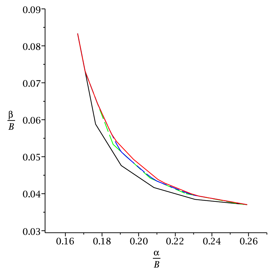
Figure 1 gives outer bounds for a code. They are presented as a trade-off between and and are based on Theorem 4.2. In this case, the graph for the trade-off shows the differences more clearly than the upper bound graph with as a function of .
The lowest of the four outer bounds is the functional-repair outer bound Next we apply the theorem with the choices of [4, Proposition 2 and Theorem 1], i.e. is a singleton and is fixed. Next we allow choices with different and finally we allow of various sizes.
Example 5.1.
We illustrate the improvements for This corresponds to the vertex in the functional-repair outer bound: , The various improvements are the following. In each case we use Theorem 4.2.
Example 5.2.
Example 4.3 lists upper bounds for a code that are obtained with Theorem 4.2. In particular,
| (33) |
Here and . Theorem 3.2 applied with and gives
which yields no improvement to the bounds listed in Example 4.3. However, after exploiting nonzero mutual information among the , the theorem uses trivial estimates for each of the . In this case, together the contain five copies of , each with . Using Proposition 4.1 we can therefore improve the last bound to
0r
| (34) |
Comparing (34) and (33) at (), And (34) improves on the bounds in Example 4.3 for
References
- [1] Alexandros G. Dimakis, P. Brighten Godfrey, Yunnan Wu, Martin J. Wainwright, and Kannan Ramchandran. Network coding for distributed storage systems. IEEE Trans. Inf. Theor., 56(9):4539–4551, September 2010.
- [2] Alexandros G. Dimakis, Kannan Ramchandran, Yunnan Wu, and Changho Suh. A survey on network codes for distributed storage. Proceedings of the IEEE, 99(3):476–489, 2011.
- [3] Korlakai Vinayak Rashmi, Nihar B. Shah, and P. Vijay Kumar. Optimal exact-regenerating codes for distributed storage at the msr and mbr points via a product-matrix construction. IEEE Transactions on Information Theory, 57(8):5227–5239, 2011.
- [4] Birenjith Sasidharan, Kaushik Senthoor, and P. Vijay Kumar. An improved outer bound on the storage-repair-bandwidth tradeoff of exact-repair regenerating codes. CoRR, abs/1312.6079, 2013.
- [5] Nihar B. Shah, K. V. Rashmi, P. Vijay Kumar, and Kannan Ramchandran. Regenerating codes for distributed storage networks. In Arithmetic of finite fields, volume 6087 of Lecture Notes in Comput. Sci., pages 215–223. Springer, Berlin, 2010.
- [6] Nihar B. Shah, K. V. Rashmi, P. Vijay Kumar, and Kannan Ramchandran. Distributed storage codes with repair-by-transfer and nonachievability of interior points on the storage-bandwidth tradeoff. IEEE Transactions on Information Theory, 58(3):1837–1852, 2012.
- [7] Chao Tian. Characterizing the rate region of the (4, 3, 3) exact-repair regenerating codes. IEEE Journal on Selected Areas in Communications, 32(5):967–975, 2014.