跳到论文正文
W Papers独立论文阅读器 arXiv:1406.4630 论文正文 计算阅读时间 · 0%
引用这篇论文根据当前论文元数据生成,正式投稿前建议核对。


License: arXiv.org perpetual non-exclusive license
arXiv:1406.4630v2 [hep-ph] 17 Sep 2014

Chiral spirals from noncontinuous chiral symmetry:
The Gross-Neveu model results

Toru Kojo Affiliation: Department of Physics, University of Illinois, 1110 West Green Street, Urbana, Illinois 61801, USA
August 24, 2026
Abstract

It is shown that the inhomogeneous chiral condensate in the Gross-Neveu (GN) model takes the chiral spiral form, even though the thermodynamic functional depends only on the chiral scalar density. It is the inhomogeneity of the chiral scalar condensate that drives the spatial modulations of the pseudoscalar one. The result has broader implications once we start to think of fundamental theories behind the effective models. In particular, some effective interactions—which may be omitted for descriptions of the homogeneous phases—can be dynamically enhanced due to the spatial modulations of the large mean fields. Implications for the four-dimensional counterparts of the GN model are discussed. In a quark matter context, proper forms of the effective models for the inhomogeneous phases are speculated, through considerations on the Fermi-Dirac sea coupling.

I Introduction

Recently, phases of the inhomogeneous chiral condensates (IChCs) have attracted renewed attention in the quark matter context [1, 2]. A number of studies based on the NJL-type model [3, 4] as well as models with the infrared (IR) enhanced interactions [5, 6] have suggested that in some domain of moderate quark density the IChC phases are energetically more favored than the normal, chiral symmetric phase. In particular, the NJL-type model studies indicate that the phase of IChC may mask the usual first-order chiral phase transition line and its critical end point, and might change the conventional wisdom.

So far, most studies have been concentrated on the chiral condensates of the liquid crystal type, in which the condensates spatially modulate in one particular direction (say, the zz direction), while they are uniform in the other two directions. For the description of such phases, the model studies rely on the understanding of their two-dimensional counterparts: the Gross-Neveu (GN) model [8, 7] as a counterpart for the NJL4 model [3], the ’t Hooft model (QCD2) [9] for the confining model [5, 6], and the NJL2 model [10] for the extended NJL4 model with tensor 4-Fermi interactions [11]. In fact, the solutions of two-dimensional models can be naturally embedded into the four-dimensional mean field ansatz.

The inhomogeneous solutions for two-dimensional models are similar but not quite identical. The QCD2 and NJL2 models are known to have the chiral spiral ground states,

⟨ψ¯ψ⟩2​D=Δcos(2pFz),⟨ψ¯iγ0γzψ⟩2​D=Δsin(2pFz),(γ52​D=γ0γz)\langle\bar{\psi}\psi\rangle_{{\rm 2D}}=\Delta\cos\left(2p_{F}z\right)\,,~~~~~~\langle\bar{\psi}\,\mathrm{i}\gamma_{0}\gamma_{z}\psi\rangle_{{\rm 2D}}=\Delta\sin\left(2p_{F}z\right)\,,~~~~(\gamma^{{\rm 2D}}_{5}=\gamma_{0}\gamma_{z}) (1)

which can be directly brought into its four-dimensional version by replacing (γ0​γz)2​D→(γ0​γz)4​D\left(\gamma_{0}\gamma_{z}\right)^{{\rm 2D}}\rightarrow\left(\gamma_{0}\gamma_{z}\right)^{{\rm 4D}}. (This solution should not be confused with the pionic chirals such as ⟨ψ¯​i​γ5​ψ⟩4​D\langle\bar{\psi}\,\mathrm{i}\gamma_{5}\psi\rangle_{{\rm 4D}} or ⟨ψ¯​i​τ3​γ5​ψ⟩4​D\langle\bar{\psi}\,\mathrm{i}\tau_{3}\gamma_{5}\psi\rangle_{{\rm 4D}} where γ54​D≠(γ0​γz)4​D\gamma_{5}^{{\rm 4D}}\neq\left(\gamma_{0}\gamma_{z}\right)^{{\rm 4D}} 11 1 The chiral spirals made of the chiral scalar and tensor condensates are dominated by pairs of particle-holes near the Fermi surface, and produce gaps. In contrast, the pionic chiral spirals in addition contain particle-antiparticle pairing, and have gaps in both the Fermi and Dirac seas. Discussions in Sec. IV can be used to understand differences between these two types of chiral spirals. .) Here 2​pF2p_{F} appears because of the condensed pairs of comoving particle-holes near the Fermi surface. On the other hand, for the GN model, the spiral solution is usually not considered, because the 4-Fermi interaction takes the form (ψ¯​ψ)2(\bar{\psi}\psi)^{2}, so that its mean-field thermodynamic functional depends only on ⟨ψ¯​ψ⟩\langle\bar{\psi}\psi\rangle but not on ⟨ψ¯​i​γ5​ψ⟩\langle\bar{\psi}\mathrm{i}\gamma_{5}\psi\rangle. Therefore, the above two classes of solutions are usually distinguished.

In this paper we explain how to understand differences between them by revisiting inhomogeneous solutions of the GN model [7]. To avoid confusion, we emphasize that we will not attempt to modify the analytic solution, which was shown to achieve the ground state [8]. On the other hand, there are physical implications which cannot be observed from the expression of the thermodynamic functional. In fact, not all condensates manifestly appear in the energy minimization procedure.

Using the analytically known fermion eigenstates, we compute condensates explicitly to show that the inhomogeneous condensate in the GN model actually takes the chiral spiral form. It is, however, not identical with those in QCD2 (NJL2). In the GN model, the net contribution to the chiral scalar density comes from the Dirac sea, while that for the chiral pseudoscalar density comes from the Fermi sea. This introduces disparities in amplitudes of two densities.

This chiral spiral solution in the GN model can be elevated to the NJL4 model. Like the GN model case, the corresponding chiral spiral–which is made of ⟨ψ¯​ψ⟩4​D\langle\bar{\psi}\psi\rangle_{{\rm 4D}} and ⟨ψ¯​i​γ0​γz​ψ⟩4​D\langle\bar{\psi}\,\mathrm{i}\gamma_{0}\gamma_{z}\psi\rangle_{{\rm 4D}}–cannot be observed from the thermodynamic functional in the NJL4 model, and it must be computed using the fermion bases in the scalar mean field of Ref. [3]. We will show the explicit mapping from two to four dimensions in another publication, but we think that the main features should already be clear from our two-dimensional analyses in this paper.

Actually, for the discussions of the QCD phase diagram, the derivation of the chiral spirals in the NJL4 model is not the end of the story. It leads to broader implications once we start to think of fundamental theories behind the effective models.

For the NJL4 model up to dimension-6 operators, in principle we should include all possible 4-Fermi interactions that are compatible with symmetries of QCD, although many of them can be discarded based on other set of arguments. For example, in vacuum, it does not matter whether or not we include tensor type interactions ∼(ψ¯​σμ​ν​ψ)2+(ψ¯​i​γ5​σμ​ν​τa​ψ)2\sim\left(\bar{\psi}\sigma_{\mu\nu}\psi\right)^{2}+\left(\bar{\psi}\mathrm{i}\gamma_{5}\sigma_{\mu\nu}\tau_{a}\psi\right)^{2}, simply because the tensor mean field is zero, not because the coupling constant is small (there are no reasons why the coupling should be very small). The only important mean field comes from the scalar density, so that terms ∼(ψ¯​ψ)2+(ψ¯​i​γ5​τa​ψ)2\sim(\bar{\psi}\psi)^{2}+(\bar{\psi}\mathrm{i}\gamma_{5}\tau_{a}\psi)^{2} are enough to take into account relevant dynamical effects and, at the same time, maintain the chiral symmetry.

The situation is different for inhomogeneous phases. As explained above, the spatially modulating scalar density drives the spatial modulation of the tensor mean field ⟨ψ¯​i​γ0​γz​ψ⟩\langle\bar{\psi}\mathrm{i}\gamma_{0}\gamma_{z}\psi\rangle whose amplitude is comparable to the scalar one. In this case, the relevance of the tensor-type interactions is dynamically enhanced, so we have to reanalyze the mean field solutions in the presence of such interactions. If the new mean fields turn out to generate another mean field, again we have to include the corresponding 4-Fermi interactions and reanalyze dynamics from the beginning. This procedure should be repeated until we exhaust all possible dynamically enhanced 4-Fermi interactions and mean fields. After that, we can pick out the effective models for the inhomogeneous phase.

This paper is organized as follows: In Sec. II, we review the inhomogeneous mean field solution for the GN model and reproduce a number of important results in Ref. [7]. We quickly summarize basics of the elliptic functions, to the extent necessary for converting the mathematical structure into physical terminology. In Sec. III, we calculate the expectation values of various operators– in particular, pseudoscalar density. By examining its relationship with the scalar density, we show that they form the chiral spirals with unequal amplitudes. In Sec. IV, we compare the chiral spirals in the GN model to QCD2 and the NJL2 model. Section V is devoted to summary.

In Sec. II and the appendixes, we add a number of supplementary materials for Ref. [7], because the descriptions in the original paper were rather dense and hard to access for nonexperts. We try to reduce the gaps between calculations in Ref. [7]. The relevant formula to be used can be found in a handbook for mathematics [12], and its derivation can be found in Ref. [13]. Throughout this paper, we use the convention (x0,x1)=(t,x)(x^{0},x^{1})=(t,x) and gμ​ν=diag.(1,−1)g_{\mu\nu}={\rm diag.}(1,-1).

II Inhomogeneous mean fields for the Gross-Neveu model

The Gross-Neveu model with NN colors is

ℒ=ψ¯​i​∂​ψ+G 2​N​(ψ¯​ψ)2,\mathcal{L}=\bar{\psi}\,\mathrm{i}{\vtop{\halign{#\cr\hfil/\hfil\crcr$\partial$\crcr}}}\psi+\frac{G}{\,2N\,}\left(\bar{\psi}\psi\right)^{2}\,, (2)

where the sum over color indices are implicit. We consider N→∞N\rightarrow\infty for the mean field considerations. Using the auxiliary field method, we have

ℒ=ψ¯​[i​∂−M⁡(x)]​ψ−N 2​G​M2​(x).\mathcal{L}=\bar{\psi}\,\left[\,\mathrm{i}{\vtop{\halign{#\cr\hfil/\hfil\crcr$\partial$\crcr}}}-M(x)\,\right]\psi-\frac{N}{\,2G\,}M^{2}(x)\,. (3)

We are going to use the canonical approach to treat the system at finite density. The constraint will be treated in Sec. III, while in this section we just investigate properties of the eigenstates.

In Sec. II.1, we first review the mean field Ansatz and some properties of the elliptic functions. In Sec. II.2, we summarize properties of the fermion eigenstates such as relations between the energy and quasimomentum. The density of states is given in Sec. II.3. How to map the UV cutoff from the homogeneous to the inhomogeneous phase is explained in Sec. II.4.

II.1 Field equations

We first analyze the Dirac equation. The field equation is

[−iγ5∂1+M(x)γ0]ψ=ωψ.\left[-\mathrm{i}\gamma^{5}\partial_{1}+M(x)\gamma^{0}\right]\psi=\omega\psi\,. (4)

To proceed further, we choose the γ\gamma matrices and spinor bases as

γ0=−σ1,γ1=i​σ3,γ5=γ0​γ1=−σ2,ψω​(x)=[φω​(x)χω​(x)].\gamma^{0}=-\sigma_{1}\,,~~~~\gamma^{1}=\mathrm{i}\sigma_{3}\,,~~~~\gamma^{5}=\gamma^{0}\gamma^{1}=-\sigma_{2}\,,~~~~\psi_{\omega}(x)=\left[\begin{matrix}\,\varphi_{\omega}(x)\,\\ \,\chi_{\omega}(x)\,\end{matrix}\right]\,. (5)

Then the field equation takes the form

[∂1−M(x)]χ=ωφ,[−∂1−M(x)]φ=ωχ.\left[\,\partial_{1}-M(x)\,\right]\chi=\omega\varphi\,,~~~~~~~\left[\,-\partial_{1}-M(x)\,\right]\varphi=\omega\chi\,. (6)

The reason to take the above bases is that the Dirac equation with a mean field can be brought into the Lame form, whose analytic properties have been investigated (Refs. [14] and [15] are very useful). From this set of equations, we can find

[−∂2∂x2−∂M∂x+M2]​φ=ω2​φ,[−∂2∂x2+∂M∂x+M2]​χ=ω2​χ.\left[-\frac{\partial^{2}}{\partial x^{2}}-\frac{\partial M}{\partial x}+M^{2}\right]\varphi=\omega^{2}\varphi\,,~~~~~~\left[-\frac{\partial^{2}}{\partial x^{2}}+\frac{\partial M}{\partial x}+M^{2}\right]\chi=\omega^{2}\chi\,. (7)

Now we consider the ansatz proposed by Thies [7]. Its form is

M⁡(x)=𝒜​λ​sn⁡(𝒜​x|λ)​cn​(𝒜​x|λ)dn⁡(𝒜​x|λ)≡𝒜​ℳ​(ξ|λ),ξ=𝒜​x,M(x)=\mathcal{A}\lambda\,\frac{\,\mathrm{sn}(\mathcal{A}x|\lambda)\,\mathrm{cn}(\mathcal{A}x|\lambda)\,}{\mathrm{dn}(\mathcal{A}x|\lambda)}\equiv\mathcal{A}\mathcal{M}(\xi|\lambda)\,,~~~~~~\xi=\mathcal{A}x\,, (8)

where sn\mathrm{sn}, cn\mathrm{cn}, and dn\mathrm{dn} are Jacobi’s elliptic functions with the elliptic modulus λ\lambda. 𝒜\mathcal{A} and λ\lambda are variational parameters. To get feelings about the ansatz, let us briefly look at basic properties of the elliptic functions:

(i) The elliptic functions interpolate the trigonometric functions and hyperbolic functions through the elliptic parameter λ\lambda 22 2 Formulas (16.13) and (16.15) in Ref. [12].. In the λ→0\lambda\rightarrow 0 limit,

sn⁡(ξ|0)=sin⁡ξ,cn⁡(ξ|0)=cos⁡ξ,dn⁡(ξ|0)=1,\mathrm{sn}(\xi|0)=\sin\xi\,,~~~\mathrm{cn}(\xi|0)=\cos\xi\,,~~~\mathrm{dn}(\xi|0)=1\,, (9)

and in the λ→1\lambda\rightarrow 1 limit,

sn⁡(ξ|1)=tanh⁡ξ,cn⁡(ξ|1)=sech​ξ,dn⁡(ξ|1)=sech​ξ,\mathrm{sn}(\xi|1)=\tanh\xi\,,~~~\mathrm{cn}(\xi|1)={\rm sech}\,\xi\,,~~~\mathrm{dn}(\xi|1)={\rm sech}\,\xi\,, (10)

with which

ℳ⁡(ξ|λ→0)∼λ2​sin⁡(2​ξ),ℳ⁡(ξ|λ→1)∼±tanh⁡(ξ).\mathcal{M}(\xi|\lambda\rightarrow 0)\sim\frac{\,\lambda\,}{2}\sin(2\xi)\,,~~~~~~\mathcal{M}(\xi|\lambda\rightarrow 1)\sim\pm\tanh(\xi)\,. (11)

The λ→0\lambda\rightarrow 0 limit corresponds to the density wave solution at high density, and the λ→1\lambda\rightarrow 1 limit corresponds to solitonic solutions at low density. As an example, in Fig.1 we plot these functions for λ=0.6\lambda=0.6. This asymptotic behavior motivates us to use the ansatz interpolating these two solutions which are known to minimize the thermodynamic potential.

Refer to caption
Figure 1: The Jacobi elliptic functions, sn⁡(ξ|λ),cn⁡(ξ|λ)\mathrm{sn}(\xi|\lambda),\,\mathrm{cn}(\xi|\lambda), and dn⁡(ξ|λ)\mathrm{dn}(\xi|\lambda) at λ=0.6\lambda=0.6. 𝐊⁡(λ){\bf K}(\lambda) is the quarter period.
Refer to caption
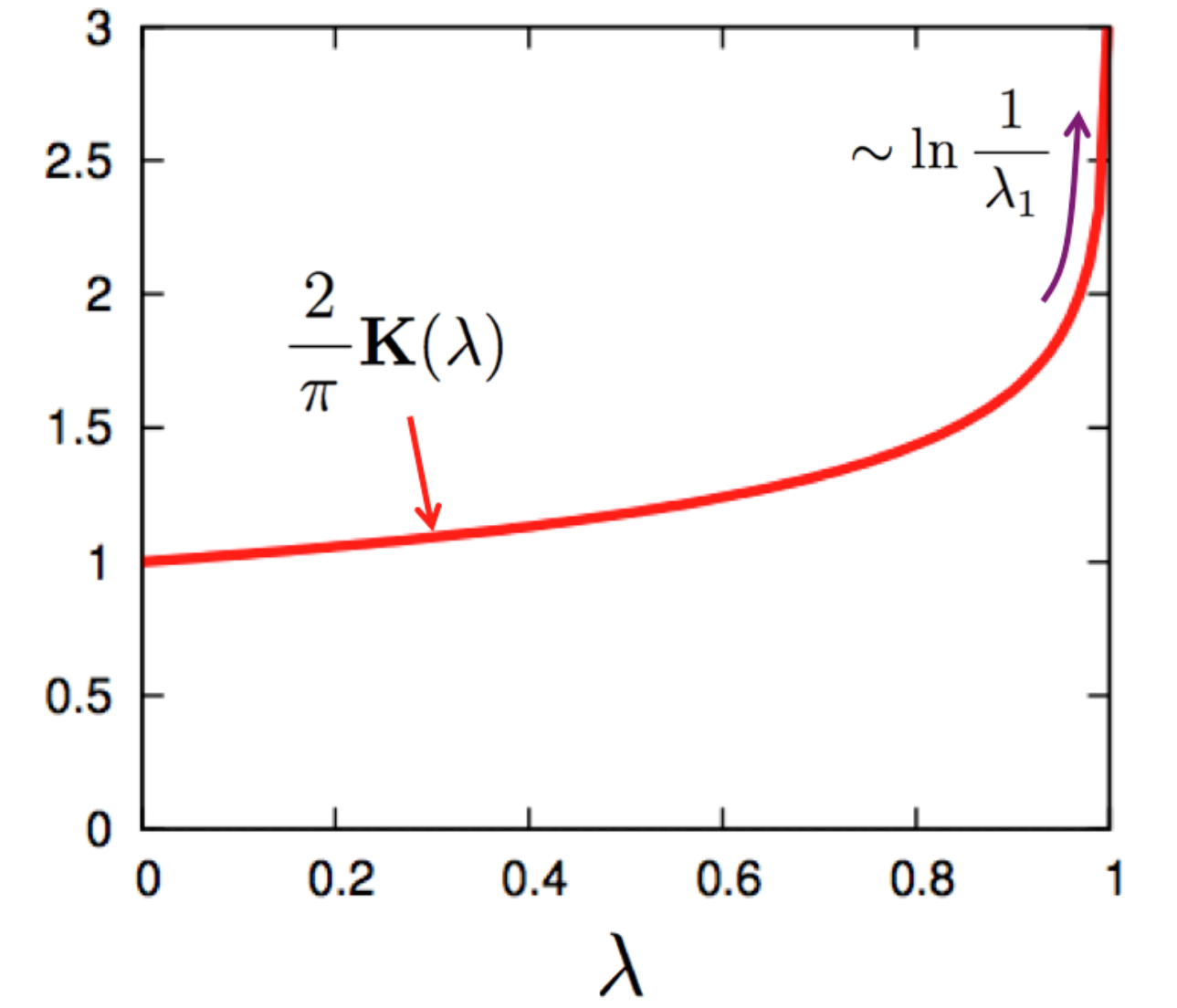
Figure 2: The Jacobi complete elliptic function of the first kind 𝐊⁡(λ){\bf K}(\lambda) (normalized by π/2\pi/2). The period grows logarithmically as λ\lambda approaches 11, which corresponds to the dilute limit of the fermion density.

(ii) As with trigonometric functions, there are simple square relations,

sn2​(ξ|λ)+cn2​(ξ|λ)=1,dn2​(ξ|λ)=1−λ​sn2​(ξ|λ).\mathrm{sn}^{2}(\xi|\lambda)+\mathrm{cn}^{2}(\xi|\lambda)=1\,,~~~~~~\mathrm{dn}^{2}(\xi|\lambda)=1-\lambda\,\mathrm{sn}^{2}(\xi|\lambda)\,. (12)

(iii) As with trigonometric functions, we can define the quarter period. It is given by the Jacobi complete elliptic integral of the first kind 33 3 Formulas (17.3.1) and (17.3.26) in Ref. [12].,

𝐊(λ)=∫0π/2d​θ1−λ​sin2⁡θ→{π/2(λ→0)1 2​ln⁡ 16λ1(λ→1),{\bf K}(\lambda)=\int^{\pi/2}_{0}\!\frac{\mathrm{d}\theta}{\,\sqrt{1-\lambda\sin^{2}\theta\,}\,}~~~~~\rightarrow~~~\left\{\begin{matrix}~~~~~\pi/2~~~~~~~(\lambda\rightarrow 0)\\ ~~\frac{1}{\,2\,}\ln\frac{\,16\,}{\,\lambda_{1}\,}~~~~~(\lambda\rightarrow 1)\end{matrix}\right.\,, (13)

where λ1≡1−λ\lambda_{1}\equiv 1-\lambda is called the complementary modulus of λ\lambda. As the name suggests, sn⁡(ξ+4​𝐊)=sn⁡(ξ)\mathrm{sn}(\xi+4{\bf K})=\mathrm{sn}(\xi), cn⁡(ξ+4​𝐊)=cn⁡(ξ),⋯\mathrm{cn}(\xi+4{\bf K})=\mathrm{cn}(\xi),\cdots are satisfied for any values of λ\lambda. The changes for the quarter period are more nontrivial, and there are formulas. 44 4 See also Table (16.8) in Ref. [12]. (Below, we sometimes omit λ\lambda as long as it does not bring any confusion.)

sn⁡(ξ±𝐊)=±cn⁡(ξ)dn⁡(ξ),cn⁡(ξ±𝐊)=∓λ11/2​sn⁡(ξ)dn⁡(ξ),dn⁡(ξ±𝐊)=λ11/2​1dn⁡(ξ),\mathrm{sn}(\xi\pm{\bf K})=\pm\frac{\,\mathrm{cn}(\xi)\,}{\,\mathrm{dn}(\xi)\,}\,,~~~~~\mathrm{cn}(\xi\pm{\bf K})=\mp\lambda_{1}^{1/2}\frac{\,\mathrm{sn}(\xi)\,}{\,\mathrm{dn}(\xi)\,}\,,~~~~~\mathrm{dn}(\xi\pm{\bf K})=\lambda_{1}^{1/2}\frac{1}{\,\mathrm{dn}(\xi)\,}\,, (14)

with which we can show

ℳ⁡(ξ)=−ℳ⁡(ξ±𝐊)=ℳ⁡(ξ±2​𝐊).\mathcal{M}(\xi)=-\mathcal{M}(\xi\pm{\bf K})=\mathcal{M}(\xi\pm 2{\bf K})\,. (15)

The first equality can be used to cast the equation for χ\chi into the same form as for φ\varphi. For later convenience, we rescale variables as

(φ⁡(x),χ⁡(x))≡(φ~​(𝒜−1​x),χ~​(𝒜−1​x))=(φ~​(ξ),χ~​(ξ)),ω~≡ω/𝒜\left(\,\varphi(x),\,\chi(x)\,\right)\equiv(\,\tilde{\varphi}(\mathcal{A}^{-1}x),\,\tilde{\chi}(\mathcal{A}^{-1}x)\,)=(\,\tilde{\varphi}(\xi),\,\tilde{\chi}(\xi)\,)\,,~~~~~~\tilde{\omega}\equiv\omega/\mathcal{A} (16)

and using Eq.(15), we can rewrite Eq.(7) as

[−∂2∂ξ2−∂ℳ⁡(ξ)∂ξ+ℳ2​(ξ)]​f​(ξ)=ω~2​f​(ξ),f⁡(ξ)=(φ~​(ξ),χ~​(ξ±𝐊)).\left[-\frac{\partial^{2}}{\partial\xi^{2}}-\frac{\partial\mathcal{M}(\xi)}{\partial\xi}+\mathcal{M}^{2}(\xi)\right]f(\xi)=\tilde{\omega}^{2}\,f(\xi)\,,~~~~~~~~f(\xi)=\left(\,\tilde{\varphi}(\xi),\,\tilde{\chi}(\xi\pm{\bf K})\,\right)\,. (17)

Note that φ~​(ξ)\tilde{\varphi}(\xi) and χ~​(ξ±𝐊)\tilde{\chi}(\xi\pm{\bf K}) satisfy the same equations, so one of the solutions can be related to the other by shifting the coordinate by 𝐊{\bf K}, modulo the relative phase factor.

(iv) The derivatives of the elliptic functions are given by 55 5 See also the Table (16.16) in Ref. [12].

d​sn​(ξ)d​ξ=cn⁡(ξ)​dn​(ξ),d​cn​(ξ)d​ξ=−sn⁡(ξ)​dn​(ξ),d​dn​(ξ)d​ξ=−λ​sn​(ξ)​cn​(ξ),\frac{\,\mathrm{d}\,\mathrm{sn}(\xi)\,}{\,\mathrm{d}\xi\,}=\mathrm{cn}(\xi)\,\mathrm{dn}(\xi)\,,~~~\frac{\,\mathrm{d}\,\mathrm{cn}(\xi)\,}{\,\mathrm{d}\xi\,}=-\mathrm{sn}(\xi)\,\mathrm{dn}(\xi)\,,~~~\frac{\,\mathrm{d}\,\mathrm{dn}(\xi)\,}{\,\mathrm{d}\xi\,}=-\lambda\,\mathrm{sn}(\xi)\,\mathrm{cn}(\xi)\,, (18)

with which one gets

d​ℳ​(ξ)d​ξ=−2​λ​sn2​(ξ)+λ+ℳ2.\frac{\,\mathrm{d}\,\mathcal{M}(\xi)\,}{\,\mathrm{d}\xi\,}=-2\lambda\,\mathrm{sn}^{2}(\xi)+\lambda+\mathcal{M}^{2}\,. (19)

Finally, we arrive at the Lame form of the eigenvalue equation:

[−∂2∂ξ2+2​λ​sn2​(ξ)]​f​(ξ)=(ω~2+λ)​f​(ξ).\left[\,-\frac{\partial^{2}}{\partial\xi^{2}}+2\lambda\,\mathrm{sn}^{2}(\xi)\,\right]f(\xi)=\left(\tilde{\omega}^{2}+\lambda\right)f(\xi)\,. (20)

The number 22 in front of sn2​(ξ)\mathrm{sn}^{2}(\xi) is the special case of l⁡(l+1)l(l+1). For given ll, the equation has 2​l2l gaps in the energy spectra [13].

II.2 Eigenvalues and eigenfunctions

To study the eigenstates, let us first note that the period of the potential is 2​𝐊​(λ)2{\bf K}(\lambda). Therefore the eigenfunction must take the Bloch form:

ΨQ​(ξ)=vQ​(ξ)​ei​Q~​ξ,vQ​(ξ)=vQ​(ξ+2​𝐊),\Psi_{Q}(\xi)=v_{Q}(\xi)\,\mathrm{e}^{\mathrm{i}\tilde{Q}\xi}\,,~~~~v_{Q}(\xi)=v_{Q}(\xi+2{\bf K})\,, (21)

where Q~=Q/𝒜\tilde{Q}=Q/\mathcal{A} is the (dimensionless) quasimomentum which is a real, continuous variable. On the other hand, the Fourier modes for vQ​(ξ)v_{Q}(\xi) can take only discrete values, n​π/𝐊n\pi/{\bf K}, where nn is an integer. Note also that the equation is the second-order differential one, and its kernel is real, so that we have a pair of solutions (φ~,χ~)(\tilde{\varphi},\tilde{\chi}), and (φ~∗,χ~∗)(\tilde{\varphi}^{*},\tilde{\chi}^{*}).

Explicitly, the solution of the Lame equation for l=1l=1 is given by [13, 14]

fα​(ξ|λ)=θ1​(uξ+α,q|λ)θ4​(uξ,q|λ)​eξ​Z​(α|λ),fα∗​(ξ|λ)=θ1∗​(uξ+α,q|λ)θ4​(uξ,q|λ)​eξ​Z∗​(α|λ),f_{\alpha}\left(\xi|\lambda\right)=\frac{\,\theta_{1}\left(u_{\xi+\alpha},q|\lambda\right)\,}{\theta_{4}\left(u_{\xi},q|\lambda\right)}\,\mathrm{e}^{\xi Z(\alpha|\lambda)}\,,~~~~~~f_{\alpha}^{*}\left(\xi|\lambda\right)=\frac{\,\theta^{*}_{1}\left(u_{\xi+\alpha},q|\lambda\right)\,}{\theta_{4}\left(u_{\xi},q|\lambda\right)}\,\mathrm{e}^{\xi Z^{*}(\alpha|\lambda)}\,, (22)

where θa​(uξ,q)\theta_{a}(u_{\xi},q) and Z⁡(α|λ)Z(\alpha|\lambda) are Jacobi ellliptic theta and zeta functions with the modulus λ\lambda, and the variables uξu_{\xi} and qq (called “nome”) are

uξ≡π​ξ 2​𝐊​(λ)→{ξ(λ→0)π​ξln⁡16λ1(λ→1),q≡e−π𝐊′/𝐊→{λ 16(λ→0)e−π2ln⁡(16/λ1)​(λ→1),u_{\xi}\equiv\frac{\pi\xi}{\,2{\bf K}(\lambda)\,}~\rightarrow~\left\{\begin{matrix}~~~~\xi~~~~~~~(\lambda\rightarrow 0)\\ ~~\frac{\pi\xi}{\,\ln\frac{16}{\lambda_{1}}\,}~~~~(\lambda\rightarrow 1)\end{matrix}\right.\,,~~~~~q\equiv\mathrm{e}^{-\pi{\bf K}^{\prime}/{\bf K}}~\rightarrow~\left\{\begin{matrix}~~~\frac{\lambda}{\,16\,}~~~~~~~(\lambda\rightarrow 0)\\ ~\mathrm{e}^{-\frac{\pi^{2}}{\ln(16/\lambda_{1})}}~~(\lambda\rightarrow 1)\end{matrix}\right.\,, (23)

where 𝐊′=𝐊′​(λ)=𝐊⁡(λ1){\bf K}^{\prime}={\bf K}^{\prime}(\lambda)={\bf K}(\lambda_{1}). Below we convert the abstract expressions into physical notions.

(i) The parameter α\alpha is directly related to the energy spectra by the following relation:

dn2​(α|λ)=ω~2.\mathrm{dn}^{2}(\alpha|\lambda)=\tilde{\omega}^{2}\,. (24)

As we shall discuss below, there is restriction on the values of α\alpha, so dn2​(α|λ)\mathrm{dn}^{2}(\alpha|\lambda) cannot take arbitrary values. Accordingly, there are forbidden regions for ω~\tilde{\omega} which appear as the energy gaps in the spectra.

(ii) We can identify the Bloch periodic function and quasimomentum as

vQ​(ξ)≡θ1​(uξ+α,q|λ)θ4​(uξ,q|λ)​exp⁡−i​π​ξ2​𝐊,Q~≡−i​Z​(α|λ)+π 2​𝐊,v_{Q}(\xi)\equiv\frac{\,\theta_{1}\left(u_{\xi+\alpha},q|\lambda\right)\,}{\theta_{4}\left(u_{\xi},q|\lambda\right)}\,\exp\frac{\,-\mathrm{i}\pi\xi\,}{2{\bf K}}\,,~~~~~~~\tilde{Q}\equiv-\mathrm{i}Z(\alpha|\lambda)+\frac{\,\pi\,}{\,2{\bf K}\,}\,, (25)

which satisfy the condition vQ=vQ+2​𝐊v_{Q}=v_{Q+2{\bf K}}. To understand this decomposition, we note that the series expansions for Jacobi ellliptic theta functions are 66 6 Formula (16.27) in Ref. [12].

θ1​(u,q)\displaystyle\theta_{1}(u,q) =2​q1/4​∑n=0∞(−1)n​qn⁡(n+1)​sin⁡(2​n+1)​u,θ1​(u)=θ1∗​(u∗)\displaystyle=2q^{1/4}\sum_{n=0}^{\infty}(-1)^{n}q^{n(n+1)}\sin(2n+1)u\,,~~~~~~~\theta_{1}(u)=\theta^{*}_{1}(u^{*})
θ4​(u,q)\displaystyle\theta_{4}(u,q) =1+2​∑n=1∞(−1)n​qn2​cos⁡2​n​u,\displaystyle=1+2\sum_{n=1}^{\infty}(-1)^{n}q^{n^{2}}\cos 2nu\,, (26)

from which we can verify

θ1​(uξ+u2​𝐊)=θ1​(uξ+π)=−θ1​(uξ),θ4​(uξ+u2​𝐊)=θ4​(uξ).\theta_{1}(u_{\xi}+u_{2{\bf K}})=\theta_{1}(u_{\xi}+\pi)=-\theta_{1}(u_{\xi})\,,~~~~~~~\theta_{4}(u_{\xi}+u_{2{\bf K}})=\theta_{4}(u_{\xi})\,. (27)

The sign flipping in the first relation is the reason why we had to include e−iπξ/2𝐊\mathrm{e}^{-\mathrm{i}\pi\xi/2{\bf K}} in vQv_{Q}.

Refer to caption
Figure 3: The dispersion relation between the energy ω~\tilde{\omega} and quasimomentum Q~\tilde{Q} (normalized by 𝒜\mathcal{A}). λ\lambda is chosen to be 0.60.6. The gap is opened at the quasimomentum π/2​𝐊\pi/2{\bf K} (η=0\eta=0), which should be assigned as p~F\tilde{p}_{F}. The energy at the band edge is ω~F=λ1\tilde{\omega}_{F}=\sqrt{\lambda_{1}} (OPENω~F′=1)\tilde{\omega}_{F}^{\prime}=1) for the first (second) energy branch. The plot is symmetric with respect to ω~→−ω~\tilde{\omega}\rightarrow-\tilde{\omega}, and the Dirac sea also has an energy gap of the same size.

(iii) The quasimomentum Q~\tilde{Q} must be a real variable, so Z⁡(α|λ)Z(\alpha|\lambda) must be purely imaginary. This constrains the value of α\alpha. The series expansion of the zeta function takes the form 77 7 Formula (17.4.38) in Ref. [12].

Z⁡(α|λ)=2​π𝐊​∑n=1∞qn 1−q2​n​sin⁡(n​π𝐊​α),Z(\alpha|\lambda)=\frac{2\pi}{\,{\bf K}\,}\sum_{n=1}^{\infty}\frac{q^{n}}{\,1-q^{2n}\,}\,\sin\left(\frac{\,n\pi\,}{{\bf K}}\,\alpha\right)\,, (28)

which has periodicity 2​𝐊2{\bf K} in α\alpha. Thus α\alpha must take the form 88 8 When η\eta exceeds 𝐊′{\bf K}^{\prime}, q​eπ​η/𝐊=eπ⁡(−𝐊′+η)/𝐊>1q\mathrm{e}^{\pi\eta/{\bf K}}=\mathrm{e}^{\pi(-{\bf K}^{\prime}+\eta)/{\bf K}}>1, and power series in Eq.(28) blow up. Thus, η∈[ 0,𝐊′]\eta\in[\,0,\,{\bf K}^{\prime}\,].

α=i​η,α=𝐊+i​η,η∈[ 0,𝐊′].\alpha=\mathrm{i}\eta\,,~~~~~~\alpha={\bf K}+\mathrm{i}\eta\,,~~~~~~\eta\in[\,0,\,{\bf K}^{\prime}\,]\,. (29)

Note that at η=0\eta=0 we have Z⁡(0)=Z⁡(𝐊)=0Z(0)=Z({\bf K})=0, meaning that the quasimomenta of two branches coincide. This is the momentum where the energy gap appears; see Fig. 3. As we will see later, to minimize the energy of the system, the quasimomentum at the gap should be taken to be pF/𝒜p_{F}/\mathcal{A},

Q~=π/2​𝐊=pF/𝒜,(η=0)\tilde{Q}=\pi/2{\bf K}=p_{F}/\mathcal{A}\,,~~~~(\eta=0) (30)

so that the first positive energy branch is perfectly filled while the second positive energy branch is empty. This determines 𝒜\mathcal{A} as a function of λ\lambda.

(iv) The energy branches are determined as follows. We first examine α=i​η\alpha=\mathrm{i}\eta (second energy branch). Using Jacobi’s imaginary transformation 99 9 Formula (16.20) in Ref. [12].,

dn⁡(i​η|λ)=dn⁡(η|λ1)cn⁡(η|λ1),\mathrm{dn}(\mathrm{i}\eta|\lambda)=\frac{\,\mathrm{dn}(\eta|\lambda_{1})\,}{\,\mathrm{cn}(\eta|\lambda_{1})\,}\,, (31)

(note that the modulus on the rhs is λ1=1−λ\lambda_{1}=1-\lambda), we arrive at an equation for the second energy branch,

ω~2=dn2​(η|λ1)cn2​(η|λ1)=λ1+ 1−λ1cn2​(η|λ1)≥1≡ω~F′ 2.\tilde{\omega}^{2}=\frac{\,\mathrm{dn}^{2}(\eta|\lambda_{1})\,}{\,\mathrm{cn}^{2}(\eta|\lambda_{1})\,}=\lambda_{1}+\frac{\,1-\lambda_{1}\,}{\,\mathrm{cn}^{2}(\eta|\lambda_{1})\,}~\geq~1~\equiv~\tilde{\omega}_{F}^{\prime\,2}\,. (32)

Next, we examine α=𝐊+i​η\alpha={\bf K}+\mathrm{i}\eta (first energy branch). Using the relation for the quarter period (14) and then Jacobi’s imaginary transformation (31), we get

dn⁡(𝐊+i​η|λ)=λ11/2dn⁡(i​η|λ)=λ11/2​cn⁡(η|λ1)dn⁡(η|λ1),\mathrm{dn}({\bf K}+\mathrm{i}\eta|\lambda)=\frac{\lambda_{1}^{1/2}}{\,\mathrm{dn}(\mathrm{i}\eta|\lambda)\,}=\lambda_{1}^{1/2}\frac{\,\mathrm{cn}(\eta|\lambda_{1})\,}{\,\mathrm{dn}(\eta|\lambda_{1})\,}\,, (33)

and then we arrive at an equation for the first energy branch,

ω~2=λ1​cn2​(η|λ1)dn2​(η|λ1)=1− 1−λ1dn2​(η|λ1)≤λ1≡ω~F2.\tilde{\omega}^{2}=\lambda_{1}\frac{\,\mathrm{cn}^{2}(\eta|\lambda_{1})\,}{\,\mathrm{dn}^{2}(\eta|\lambda_{1})\,}=1-\frac{\,1-\lambda_{1}\,}{\,\mathrm{dn}^{2}(\eta|\lambda_{1})\,}~\leq~\lambda_{1}~\equiv~\tilde{\omega}_{F}^{2}\,. (34)

Therefore we find the energy gap between edges of the two branches, ω~F2=λ1\tilde{\omega}_{F}^{2}=\lambda_{1} and ω~F′ 2=1\tilde{\omega}_{F}^{\prime\,2}=1. Because the relation is given for ω~2\tilde{\omega}^{2}, we have the gaps not only near the Fermi points but also in the Dirac sea. The energies as functions of quasimomenta are plotted in Fig.3.

(v) In the following calculations, we assign eigenfunctions for φ~\tilde{\varphi} and φ~∗\tilde{\varphi}^{*} as

φ~ω​(ξ)=𝒩​θ1​(uξ+α,q|λ)θ4​(uξ,q|λ)​eξ​Z​(α|λ),φ~ω∗​(ξ)=𝒩∗​θ1​(uξ+α∗,q|λ)θ4​(uξ,q|λ)​e−ξ​Z​(α|λ),\tilde{\varphi}_{\omega}(\xi)=\mathcal{N}\frac{\,\theta_{1}\left(u_{\xi+\alpha},q|\lambda\right)\,}{\theta_{4}\left(u_{\xi},q|\lambda\right)}\,\mathrm{e}^{\xi Z(\alpha|\lambda)}\,,~~~~~~\tilde{\varphi}_{\omega}^{*}(\xi)=\mathcal{N}^{*}\frac{\,\theta_{1}\left(u_{\xi+\alpha^{*}},q|\lambda\right)\,}{\theta_{4}\left(u_{\xi},q|\lambda\right)}\,\mathrm{e}^{-\xi Z(\alpha|\lambda)}\,, (35)

where 𝒩\mathcal{N} is the normalization factor. The relation between these two functions is like that between ei​k​x\mathrm{e}^{\mathrm{i}kx} and e−i​k​x\mathrm{e}^{-\mathrm{i}kx} in a free fermion theory. On the other hand, they are related to χω\chi_{\omega} and χω∗\chi_{\omega}^{*} through Eq.(6). Actually the results in this paper do not require the expression of the relative phase factor. But we give the result for completeness, and it is given by (for the derivation, see Appendix.B)

χ~ω​(ξ)=ei​Φ​(ω)​φ~ω​(ξ−𝐊),ei​Φ​(ω)≡sgn⁡(ω~)​e𝐊​Z​(α),\tilde{\chi}_{\omega}(\xi)=\mathrm{e}^{\mathrm{i}\Phi(\omega)}\,\tilde{\varphi}_{\omega}(\xi-{\bf K})\,,~~~~~~~\mathrm{e}^{\mathrm{i}\Phi(\omega)}\equiv{\rm sgn}(\tilde{\omega})\,\mathrm{e}^{{\bf K}Z(\alpha)}\,, (36)

where Φ\Phi is real and the function χ⁡(ξ)\chi(\xi) is proportional to φ⁡(ξ−𝐊)\varphi(\xi-{\bf K}), as stated earlier. Note also that the phase factor changes the sign for ω→−ω\omega\rightarrow-\omega, as we can see from Eq.(6).

(vi) Finally we fix the normalization. Since the wave function has periodicity of 2​𝐊2{\bf K}, the normalization condition is

1= 1 2​𝐊​∫02​𝐊d​ξ​(|φ~​(ξ)|2+|χ~​(ξ)|2)= 1 2​𝐊​∫02​𝐊d​ξ​(|φ~​(ξ)|2+|φ~​(ξ−𝐊)|2).1=\frac{\,1\,}{\,2{\bf K}\,}\int_{0}^{2{\bf K}}\mathrm{d}\xi\,~\left(\,|\tilde{\varphi}(\xi)|^{2}+|\tilde{\chi}(\xi)|^{2}\,\right)=\frac{\,1\,}{\,2{\bf K}\,}\int_{0}^{2{\bf K}}\mathrm{d}\xi\,\left(\,|\tilde{\varphi}(\xi)|^{2}+|\tilde{\varphi}(\xi-{\bf K})|^{2}\,\right)\,. (37)

We will give the explicit form of 𝒩\mathcal{N} in Appendix.C. Instead, here we give only the normalized expression for |φ~|2|\tilde{\varphi}|^{2},

|φ~ω​(ξ)|2=1 2​[ 1−dn2​(ξ)−𝐄/𝐊ω~2−𝐄/𝐊],|\tilde{\varphi}_{\omega}(\xi)|^{2}=\frac{1}{\,2\,}\left[\,1-\frac{\,\mathrm{dn}^{2}(\xi)-{\bf E}/{\bf K}\,}{\,\tilde{\omega}^{2}-{\bf E}/{\bf K}\,}\,\right]\,, (38)

where 𝐄=𝐄⁡(λ){\bf E}={\bf E}(\lambda) is the complete elliptic integral of the second kind 1010 10 Formulas (17.2), (17.3) and the figure (17.2) in Ref. [12].,

𝐄(λ)=∫0π/2dθ1−λ​sin2⁡θ=∫0𝐊dξdn2(ξ|λ)→{π/2​(λ→0)1(λ→1).{\bf E}(\lambda)=\int^{\pi/2}_{0}\!\mathrm{d}\theta\,\sqrt{1-\lambda\sin^{2}\theta\,}=\int_{0}^{{\bf K}}\!\mathrm{d}\xi~\mathrm{dn}^{2}(\xi|\lambda)~\rightarrow~\left\{\begin{matrix}~~\pi/2~~(\lambda\rightarrow 0)\\ ~~~1~~~~(\lambda\rightarrow 1)\end{matrix}\right.\,. (39)

Note that ∫02​𝐊d​ξ​[dn2​(ξ)−𝐄/𝐊]=0\int_{0}^{2{\bf K}}\mathrm{d}\xi\,[\mathrm{dn}^{2}(\xi)-{\bf E}/{\bf K}]=0, so the spatial average of |φ~|2|\tilde{\varphi}|^{2} is saturated by the first term in Eq.(38).

II.3 Density of states

In various computations we will use the density of states. We take a derivative for the quasimomentum,

d​Q~=d​Q~d​ω~​d​ω~=d​Q~d​α​d​αd​ω~​d​ω~,𝒟⁡(ω)≡|d​Q~d​ω~|.\mathrm{d}\tilde{Q}=\frac{\mathrm{d}\tilde{Q}}{\,\mathrm{d}\tilde{\omega}\,}\,\mathrm{d}\tilde{\omega}=\frac{\mathrm{d}\tilde{Q}}{\,\mathrm{d}\alpha\,}\frac{\mathrm{d}\alpha}{\,\mathrm{d}\tilde{\omega}\,}\,\mathrm{d}\tilde{\omega}\,,~~~~~\mathcal{D}(\omega)\equiv\left|\frac{\mathrm{d}\tilde{Q}}{\,\mathrm{d}\tilde{\omega}\,}\right|\,. (40)

The α\alpha and ω~\tilde{\omega} are related through the relation (24). Let us first note that

dd​ω~​dn​(α)=dd​ω~​ω~↔d​αd​ω~=1λ​1sn⁡(α)​cn​(α),\frac{\mathrm{d}}{\,\mathrm{d}\tilde{\omega}\,}\,\mathrm{dn}(\alpha)=\frac{\mathrm{d}}{\,\mathrm{d}\tilde{\omega}\,}\,\tilde{\omega}~~~\leftrightarrow~~~\frac{\mathrm{d}\alpha}{\,\mathrm{d}\tilde{\omega}\,}=\frac{1}{\,\lambda\,}\frac{1}{\,\mathrm{sn}(\alpha)\,\mathrm{cn}(\alpha)\,}\,, (41)

where either sn⁡(α)\mathrm{sn}(\alpha) or cn⁡(α)\mathrm{cn}(\alpha) becomes purely imaginary. Next we deal with d​Q~/d​α\mathrm{d}\tilde{Q}/\mathrm{d}\alpha. Taking a derivative of the dispersion relation (see Appendix.D), we find

d​Q~d​α=−i​d​Z​(α)d​α=−i⁡(dn2​(α)−𝐄𝐊).\frac{\mathrm{d}\tilde{Q}}{\,\mathrm{d}\alpha\,}=-\mathrm{i}\frac{\,\mathrm{d}Z(\alpha)\,}{\,\mathrm{d}\alpha\,}=-\mathrm{i}\left(\mathrm{dn}^{2}(\alpha)-\frac{{\bf E}}{{\bf K}}\right)\,. (42)

Assembling all these pieces, we arrive at

𝒟(ω)=∓ω~2−𝐄/𝐊(ω~2−1)​(ω~2−λ1).(−for0≤ω~2≤λ1,+for1≤ω~2)\mathcal{D}(\omega)=\mp\,\frac{\,\tilde{\omega}^{2}-{\bf E}/{\bf K}\,}{\sqrt{(\tilde{\omega}^{2}-1)(\tilde{\omega}^{2}-\lambda_{1})\,}\,}\,.~~~~\left(-~{\rm for}~0\leq\,\tilde{\omega}^{2}\leq\lambda_{1}\,,~+~{\rm for}~1\leq\tilde{\omega}^{2}\,\right) (43)

Note that ω~2=𝐄/𝐊\tilde{\omega}^{2}={\bf E}/{\bf K} is in the forbidden region between the first and second energy branches. In fact there is an inequality λ1≤𝐄/𝐊≤1\lambda_{1}\leq{\bf E}/{\bf K}\leq 1 which can be derived by noting that λ1≤dn2​x≤1\lambda_{1}\leq\mathrm{dn}^{2}x\leq 1 and ∫0𝐊d​x​dn2​(x)=𝐄\int^{{\bf K}}_{0}\mathrm{d}x~\mathrm{dn}^{2}(x)={\bf E}. Note that the density of states is enhanced near the band edges.

II.4 Mapping of the UV cutoff

Finally, we relate the UV cutoff. Details will be given in Appendix.E, but we will give the outline here. First, we notice that dn⁡(α)\mathrm{dn}(\alpha) for α=i​η\alpha=\mathrm{i}\eta approaches +∞+\infty as α→i​𝐊′​(λ)\alpha\rightarrow\mathrm{i}{\bf K}^{\prime}(\lambda). Introducing an infinitesimal quantity ϵ\epsilon, our energy cutoff for the inhomogenous phase, ωΛ\omega_{\Lambda}, can be expressed as

ωΛ/𝒜=dn⁡(i⁡(𝐊′−ϵ)|λ).\omega_{\Lambda}/\mathcal{A}=\mathrm{dn}\left(\,\mathrm{i}({\bf K}^{\prime}-\epsilon)|\lambda\,\right)\,. (44)

On the other hand, the number of states in the Dirac sea is limited by k=Λk=\Lambda. Using the expression for the quasimomentum, we can write the momentum cutoff as

Λ/𝒜=−i​Z​(i⁡(𝐊′−ϵ)|λ)+π 2​𝐊​(λ).\Lambda/\mathcal{A}=-\mathrm{i}Z\left(\,\mathrm{i}({\bf K}^{\prime}-\epsilon)|\lambda\,\right)+\frac{\,\pi\,}{\,2{\bf K}(\lambda)\,}\,. (45)

Expanding these equations by ϵ\epsilon, we can eliminate ϵ\epsilon and then relate the momentum cutoff to the energy cutoff,

ωΛ2=Λ2+𝒜2​[−λ+2​( 1−𝐄𝐊)]+O⁡(Λ−2).\omega^{2}_{\Lambda}=\Lambda^{2}+\mathcal{A}^{2}\,\left[\,-\lambda+2\left(\,1-\frac{{\bf E}}{\,{\bf K}\,}\,\right)\,\right]+O(\Lambda^{-2})\,. (46)

The O⁡(1)O(1) terms must be kept during the following calculations.

III Expectation values

Now we have all the ingredients to compute various quantities. We first write down expressions for the fermion number density and energy density, and then determine the variational parameters 𝒜\mathcal{A} and λ\lambda as functions of average density or pFp_{F}. After that we compute the spatial modulations of various density operators: fermion number, energy, and scalar and pseudoscalar density. At the end of this section, in Sec. III.5, we examine the high and low density limits of various quantities to get qualitative insights.

Using the bases found in the previous section, the fermion field operator can be written in terms of the creation and annihilation operators,

ψ^c​(x)=∫d​ω2​π​𝒟⁡(ω)​∑j=1,2uωj​(ξ)​[θ⁡(ω)​e−i​ω​t​a^c​(ω,j)+θ⁡(−ω)​ei​ω​t​b^c†​(ω,j)],\hat{\psi}_{c}(x)=\int\frac{\,\mathrm{d}\omega\,}{2\pi}\,\sqrt{\,\mathcal{D}(\omega)\,}\,\sum_{j=1,2}u^{j}_{\omega}(\xi)\left[\,\theta(\omega)\,\mathrm{e}^{-\mathrm{i}\omega t}\,\hat{a}_{c}(\omega,j)+\theta(-\omega)\,\mathrm{e}^{\mathrm{i}\omega t}\,\hat{b}_{c}^{\dagger}(\omega,j)\,\right]\,, (47)

where a^\hat{a} and b^\hat{b} are annihilation operators for particles and antiparticles, and cc is used for color indices. 𝒟⁡(ω)\mathcal{D}(\omega) is the density of states, and we took the normalization of the creation and annihilation operators to satisfy {ac​(ω,j),ac′†​(ω′,j′)}=2​π​δ​(ω−ω′)​δj​j′​δc​c′\{a_{c}(\omega,j),a_{c^{\prime}}^{\dagger}(\omega^{\prime},j^{\prime})\}=2\pi\delta(\omega-\omega^{\prime})\delta_{jj^{\prime}}\delta_{cc^{\prime}}. [This normalization requires 𝒟\sqrt{\mathcal{D}} in Eq. (47).] The wave functions giving energy ω\omega are

uω1​(ξ)=[φ~ω​(ξ)χ~ω​(ξ)],uω2​(ξ)=[φ~ω∗​(ξ)χ~ω∗​(ξ)],φ~ω=φ~−ω,χ~ω=−χ~−ω,u_{\omega}^{1}(\xi)=\left[\begin{matrix}\,\tilde{\varphi}_{\omega}(\xi)\,\\ \,\tilde{\chi}_{\omega}(\xi)\,\end{matrix}\right]\,,~~~~~u_{\omega}^{2}(\xi)=\left[\begin{matrix}\,\tilde{\varphi}^{*}_{\omega}(\xi)\,\\ \,\tilde{\chi}^{*}_{\omega}(\xi)\,\end{matrix}\right]\,,~~~~~\tilde{\varphi}_{\omega}=\tilde{\varphi}_{-\omega}\,,~~~~~\tilde{\chi}_{\omega}=-\tilde{\chi}_{-\omega}\,, (48)

where for the convention φ~ω=φ~−ω\tilde{\varphi}_{\omega}=\tilde{\varphi}_{-\omega}, the relative sign in χ~ω\tilde{\chi}_{\omega} for the positive and negative energy accompanies (−1)(-1).

III.1 Fermion number: Determination of 𝒜\mathcal{A}

The fermion number density is given by

⟨ψ†​ψ⟩=∫d​ω2​π​𝒟​(ω)​∑j=1,2|uωj​(ξ)|2​⟨θ⁡(ω)​a^†​(ω,j)​a^​(ω,j)+θ⁡(−ω)​[ 1−b^†​(ω,j)​b^​(ω,j)]⟩,\left\langle\psi^{{\dagger}}\psi\right\rangle=\int\!\frac{\,\mathrm{d}\omega\,}{2\pi}\,\mathcal{D}(\omega)\sum_{j=1,2}|u^{j}_{\omega}(\xi)|^{2}\left\langle\theta(\omega)\,\hat{a}^{\dagger}(\omega,j)\hat{a}(\omega,j)+\theta(-\omega)\left[\,1-\hat{b}^{\dagger}(\omega,j)\hat{b}(\omega,j)\right]\right\rangle\,, (49)

where the sum over color indices is implicit. Considering the fermion number constraint and the fact that the Dirac sea does not contain any antiparticles, we may require

⟨a^†​(ω,j)​a^​(ω,j)⟩=N​θ​(ϵF−ω),θ⁡(−ω)​⟨b^†​(ω,j)​b^​(ω,j)⟩=0,\left\langle\hat{a}^{\dagger}(\omega,j)\hat{a}(\omega,j)\right\rangle=N\,\theta(\epsilon_{F}-\omega)\,,~~~~~\theta(-\omega)\left\langle\hat{b}^{\dagger}(\omega,j)\hat{b}(\omega,j)\right\rangle=0\,, (50)

where ϵF\epsilon_{F} is the Fermi energy which will be fixed below. We arrive at

⟨ψ†​ψ​(x)⟩\displaystyle\left\langle\psi^{{\dagger}}\psi(x)\right\rangle =2N(∫0ϵF+∫−ωΛ0)d​ω2​π𝒟(ω)(|φ~ω(ξ)|2+|χ~ω(ξ)|2)\displaystyle=2N\left(\int_{0}^{\epsilon_{F}}+\int_{-\omega_{\Lambda}}^{0}\right)\!\frac{\,\mathrm{d}\omega\,}{2\pi}\,\mathcal{D}(\omega)\left(\,|\tilde{\varphi}_{\omega}(\xi)|^{2}+|\tilde{\chi}_{\omega}(\xi)|^{2}\,\right)
=N(∫0ϵF+∫−ωΛ0)d​ω2​π𝒟(ω)[ 2−ℱ⁡(ξ)ω2/𝒜2−𝐄/𝐊].\displaystyle=N\left(\int_{0}^{\epsilon_{F}}+\int_{-\omega_{\Lambda}}^{0}\right)\!\frac{\,\mathrm{d}\omega\,}{2\pi}\,\mathcal{D}(\omega)\left[\,2-\frac{\,\mathcal{F}(\xi)\,}{\omega^{2}/\mathcal{A}^{2}-{\bf E}/{\bf K}}\,\right]\,. (51)

where we have defined

ℱ⁡(ξ)≡dn2​(ξ)+dn2​(ξ−𝐊)−2​𝐄/𝐊,\mathcal{F}(\xi)\equiv\mathrm{dn}^{2}(\xi)+\mathrm{dn}^{2}(\xi-{\bf K})-2{\bf E}/{\bf K}\,, (52)

whose spatial average over the period 2​𝐊2{\bf K} is zero. Here we took into account the particles which fill the Dirac sea. The average part in the Dirac sea will be eliminated by the vacuum subtraction, while the spatial modulation is not and requires some care.

(i) Average density: We first compute the constant part. In order to minimize the energy, the particle should fill the first valence band, leaving the upper energy branch empty. In Appendix.F, we will show that locating the Fermi surface at the gapped points indeed reduces the energy density. Therefore, in the following, we set ϵF=ωF=λ1​𝒜\epsilon_{F}=\omega_{F}=\sqrt{\lambda_{1}}\mathcal{A}. Next, notice that we impose the UV cutoff on momenta, so the size of phase space in the Dirac sea is kept fixed. Therefore, the Dirac sea contribution to the femion number density is common for all phases. Thus, subtracting the Dirac sea contribution, we demand that

⟨ψ†​ψ​(x)⟩ave.RN=∫0ωF=λ1​𝒜d​ωπ​𝒜2​𝐄/𝐊−ω2(ω2−𝒜2)​(ω2−λ1​𝒜2)=pFπ.\frac{\,\left\langle\psi^{{\dagger}}\psi(x)\right\rangle_{{\rm ave.}}^{R}\,}{N}=\int_{0}^{\omega_{F}=\sqrt{\lambda_{1}}\mathcal{A}}\frac{\,\mathrm{d}\omega\,}{\pi}\frac{\,\mathcal{A}^{2}{\bf E}/{\bf K}-\omega^{2}\,}{\sqrt{(\omega^{2}-\mathcal{A}^{2})(\omega^{2}-\lambda_{1}\mathcal{A}^{2})\,}\,}=\frac{\,p_{F}\,}{\pi}\,. (53)

Taking the variable ω=λ1​𝒜​t\omega=\sqrt{\lambda_{1}}\mathcal{A}t, the integral can be expressed as

𝒜π​∫01d​t​[ 1−λ1​t2 1−t2− 1−𝐄/𝐊(1−t2)​(1−λ1​t2)]=𝒜π​𝐊​[𝐄′​𝐊+𝐄𝐊′−𝐊𝐊′]=𝒜 2​𝐊,\frac{\mathcal{A}}{\pi}\int_{0}^{1}\mathrm{d}t\left[\sqrt{\frac{\,1-\lambda_{1}t^{2}\,}{\,1-t^{2}\,}\,}-\frac{\,1-{\bf E}/{\bf K}\,}{\sqrt{(1-t^{2})(1-\lambda_{1}t^{2})\,}}\right]=\frac{\mathcal{A}}{\,\pi{\bf K}\,}\left[\,{\bf E}^{\prime}{\bf K}+{\bf E}{\bf K}^{\prime}-{\bf K}{\bf K}^{\prime}\,\right]=\frac{\,\mathcal{A}\,}{\,2{\bf K}\,}\,, (54)

where in the first step we used the integral expression for 𝐄′=𝐄⁡(λ1){\bf E}^{\prime}={\bf E}(\lambda_{1}) and 𝐊′=𝐊⁡(λ1){\bf K}^{\prime}={\bf K}(\lambda_{1}), and in the last step we have used Legendre’s relation. Now 𝒜\mathcal{A} is fixed to

𝒜= 2​𝐊πpF→{pF(λ→0)pFπ​ln⁡16λ1(λ→1)\mathcal{A}=\frac{\,2{\bf K}\,}{\pi}\,p_{F}~\rightarrow~\left\{\begin{matrix}~~~~~~~p_{F}~~~~~~~~(\lambda\rightarrow 0)\\ ~~~\frac{\,p_{F}\,}{\pi}\ln\frac{16}{\,\lambda_{1}\,}~~~~~(\lambda\rightarrow 1)\end{matrix}\right. (55)

Now the only remaining variational parameter is λ\lambda.

(ii) The spatially modulating part: Next, we treat the spatially modulating part (whose spatial average is zero). It is given by (see Fig. 3 for a reminder)

−N𝒜2 2​π(∫0ωF+∫−ωF0+∫−ωΛ−ωF′)dωsgn⁡(ω2−𝒜2​𝐄/𝐊)(ω2−𝒜2)​(ω2−λ1​𝒜2)ℱ(ξ).-N\frac{\,\mathcal{A}^{2}\,}{\,2\pi\,}\left(\int_{0}^{\omega_{F}}+\int_{-\omega_{F}}^{0}+\int_{-\omega_{\Lambda}}^{-\omega^{\prime}_{F}}\right)\!\mathrm{d}\omega\,\frac{{\rm sgn}\left(\omega^{2}-\mathcal{A}^{2}{\bf E}/{\bf K}\right)}{\sqrt{(\omega^{2}-\mathcal{A}^{2})(\omega^{2}-\lambda_{1}\mathcal{A}^{2})\,}}\,\mathcal{F}(\xi)\,. (56)

The integral part from the first energy branches in the Fermi (Dirac) sea gives

−∫0ωFd​ω(ω2−𝒜2)​(ω2−λ1​𝒜2)=−1𝒜∫01d​t(1−t2)​(1−λ1​t2)=−𝐊′​(λ)𝒜,-\int_{0}^{\omega_{F}}\!\frac{\,\mathrm{d}\omega\,}{\,\sqrt{(\omega^{2}-\mathcal{A}^{2})(\omega^{2}-\lambda_{1}\mathcal{A}^{2})\,}\,}=-\frac{1}{\,\mathcal{A}\,}\int_{0}^{1}\frac{\mathrm{d}t}{\,\sqrt{(1-t^{2})(1-\lambda_{1}t^{2})\,}\,}=-\frac{\,{\bf K}^{\prime}(\lambda)\,}{\mathcal{A}}\,, (57)

where we have changed the variable as ω=λ1​𝒜​t\omega=\sqrt{\lambda_{1}}\mathcal{A}t. On the other hand, the second energy branch in the Dirac sea gives a contribution with the same size but opposite sign (ωF′=𝒜\omega_{F}^{\prime}=\mathcal{A}),

∫−ωΛ−𝒜d​ω(ω2−𝒜2)​(ω2−λ1​𝒜2)=𝐊′​(λ)𝒜.\int_{-\omega_{\Lambda}}^{-\mathcal{A}}\frac{\,\mathrm{d}\omega\,}{\,\sqrt{(\omega^{2}-\mathcal{A}^{2})(\omega^{2}-\lambda_{1}\mathcal{A}^{2})\,}\,}=\frac{\,{\bf K}^{\prime}(\lambda)\,}{\mathcal{A}}\,. (58)

This can be checked by noting that the change of the variable ω→1/ω′\omega\rightarrow 1/\omega^{\prime} converts the integral into the same form as that in Eq.(57). Note that the Dirac sea contributions from the first and the second energy branches cancel out, leaving only the net contribution from the Fermi sea.

Assembling the spatial average and modulating parts, the fermion number density is given by

⟨ψ†​ψ​(x)⟩=N​pFπ​( 1+𝐊𝐊′π​ℱ​(ξ)),(ξ=𝒜​x)\left\langle\psi^{{\dagger}}\psi(x)\right\rangle=N\,\frac{\,p_{F}\,}{\pi}\left(\,1+\frac{\,{\bf K}{\bf K}^{\prime}\,}{\,\pi\,}\,\mathcal{F}(\xi)\right)\,,~~~~~(\xi=\mathcal{A}x) (59)

where we have used 𝒜=2​pF​𝐊/π\mathcal{A}=2p_{F}{\bf K}/\pi in Eq.(55). The behavior at λ=0.9\lambda=0.9 is plotted in Fig. 4.

III.2 Energy density: Determination of λ\lambda

Next we compute the energy density. The single-particle energy contribution gives

ℰ1​(x)\displaystyle\mathcal{E}_{1}(x) ≡2N(∫0ωF+∫−ωΛ0)d​ω2​π𝒟(ω)ω(|φ~ω(ξ)|2+|χ~ω(ξ)|2)\displaystyle\equiv 2N\left(\int_{0}^{\omega_{F}}+\int_{-\omega_{\Lambda}}^{0}\right)\!\frac{\,\mathrm{d}\omega\,}{2\pi}\,\mathcal{D}(\omega)\,\omega\,\left(\,|\tilde{\varphi}_{\omega}(\xi)|^{2}+|\tilde{\chi}_{\omega}(\xi)|^{2}\,\right)
=−N∫ωF′ωΛd​ω2​π𝒟(ω)ω[ 2−ℱ⁡(ξ)ω2/𝒜2−𝐄/𝐊],\displaystyle=-N\int_{\omega_{F}^{\prime}}^{\omega_{\Lambda}}\!\frac{\,\mathrm{d}\omega\,}{2\pi}\,\mathcal{D}(\omega)\,\omega\left[\,2-\frac{\,\mathcal{F}(\xi)\,}{\omega^{2}/\mathcal{A}^{2}-{\bf E}/{\bf K}}\,\right]\,, (60)

where the integrand is an odd function of ω\omega, so that Fermi and Dirac sea contributions from the first energy branches cancel, leaving the contribution from the second energy branch in the Dirac sea. (We have changed the variable as ω→−ω\omega\rightarrow-\omega.) Writing the spatial average and spatial fluctuation parts as ℰ¯1\bar{\mathcal{E}}_{1} and Δ​ℰ\Delta\mathcal{E}, straightforward calculations lead to

ℰ¯1RN\displaystyle\frac{\,\bar{\mathcal{E}}^{R}_{1}\,}{N} =−𝒜2 4​π​[(2−λ−2​𝐄𝐊)​ln⁡ 4​Λ2λ​𝒜2+(2−λ−4​𝐄𝐊)],\displaystyle=-\frac{\,\mathcal{A}^{2}\,}{\,4\pi\,}\left[\,\left(2-\lambda-2\,\frac{\,{\bf E}\,}{{\bf K}}\right)\ln\frac{\,4\Lambda^{2}\,}{\,\lambda\mathcal{A}^{2}\,}+\left(2-\lambda-4\,\frac{\,{\bf E}\,}{{\bf K}}\right)\,\right]\,,
Δ​ℰ1N\displaystyle\frac{\,\Delta\mathcal{E}_{1}\,}{N} =𝒜2 4​π​ℱ​(ξ)​ln⁡ 4​Λ2λ​𝒜2,\displaystyle=\frac{\,\mathcal{A}^{2}\,}{\,4\pi\,}\,\mathcal{F}(\xi)\ln\frac{\,4\Lambda^{2}\,}{\,\lambda\mathcal{A}^{2}\,}\,, (61)

where we define the regularized energy ℰ¯1R≡ℰ¯1−ℰvac\bar{\mathcal{E}}^{R}_{1}\equiv\bar{\mathcal{E}}_{1}-\mathcal{E}_{{\rm vac}} where ℰvac=−NΛ2/2π\mathcal{E}_{{\rm vac}}=-N\Lambda^{2}/2\pi, and drop the O⁡(1/Λ)O(1/\Lambda) terms.

Next we consider the contribution from the condensation terms. We first note that

M2​(x)𝒜2=λ2​sn2​(ξ)​cn2​(ξ)dn2​(ξ)=(2−λ−2​𝐄𝐊)−ℱ⁡(ξ),\frac{\,M^{2}(x)\,}{\mathcal{A}^{2}}=\lambda^{2}\frac{\,\mathrm{sn}^{2}(\xi)\,\mathrm{cn}^{2}(\xi)\,}{\mathrm{dn}^{2}(\xi)}=\left(2-\lambda-2\,\frac{{\bf E}}{\,{\bf K}\,}\right)-\mathcal{F}(\xi)\,, (62)

where the first bracket gives the spatial average, as we can see from the second bracket which is vanishing after averaging over the period 2​𝐊2{\bf K}. These terms have coefficient 1/G1/G whose renormalized value is determined through the renormalization condition,

1G⁡(Λ)=1 2​π​ln⁡4​Λ2M02,\frac{1}{\,G(\Lambda)\,}=\frac{1}{\,2\pi\,}\ln\frac{4\Lambda^{2}}{\,M_{0}^{2}\,}\,, (63)

where M0M_{0} is the effective mass in vacuum. With this expression, we have the average and fluctuation parts of the condensation energy (ℰ2/N≡M2​(x)/2​G\mathcal{E}_{2}/N\equiv M^{2}(x)/2G)

ℰ¯2N=𝒜2 4​π​(2−λ−2​𝐄𝐊)​ln⁡ 4​Λ2M02,Δ​ℰ2N=−𝒜2 4​π​ℱ​(ξ)​ln⁡ 4​Λ2M02.\frac{\,\bar{\mathcal{E}}_{2}\,}{N}=\frac{\,\mathcal{A}^{2}\,}{\,4\pi\,}\left(2-\lambda-2\,\frac{\,{\bf E}\,}{{\bf K}}\right)\ln\frac{\,4\Lambda^{2}\,}{\,M_{0}^{2}\,}\,,~~~~\frac{\,\Delta\mathcal{E}_{2}\,}{N}=-\frac{\,\mathcal{A}^{2}\,}{\,4\pi\,}\,\mathcal{F}(\xi)\ln\frac{\,4\Lambda^{2}\,}{\,M_{0}^{2}\,}\,. (64)

After combining ℰ1\mathcal{E}_{1} and ℰ2\mathcal{E}_{2}, we can erase Λ\Lambda in the logarithms, and the energy depends on Λ\Lambda only through the renormalized paramemeter. Now we can write down the average and fluctuating parts of total energy. The average part is

(ℰ¯1+ℰ¯2)RN=−𝒜2 4​π​[(2−λ−2​𝐄𝐊)​ln⁡M02λ​𝒜2+(2−λ−4​𝐄𝐊)],\frac{\,\left(\bar{\mathcal{E}}_{1}+\bar{\mathcal{E}}_{2}\right)_{R}\,}{N}=-\frac{\,\mathcal{A}^{2}\,}{\,4\pi\,}\left[\,\left(2-\lambda-2\,\frac{\,{\bf E}\,}{{\bf K}}\right)\ln\frac{\,M_{0}^{2}\,}{\,\lambda\mathcal{A}^{2}\,}+\left(2-\lambda-4\,\frac{\,{\bf E}\,}{{\bf K}}\right)\,\right]\,, (65)

where 𝒜=2​pF​𝐊/π\mathcal{A}=2p_{F}{\bf K}/\pi due to the fermion number constraints; see Eq. (55). We have to choose the value of λ\lambda so as to minimize the total average energy density. Using a relation

∂λ𝐄=∂λ∫01d​t​1−λ​t21−t2=𝐄−𝐊2​λ,\partial_{\lambda}{\bf E}=\partial_{\lambda}\int_{0}^{1}\mathrm{d}t\sqrt{\frac{1-\lambda t^{2}}{1-t^{2}}}=\frac{\,{\bf E}-{\bf K}\,}{2\lambda}\,, (66)

we can show that only terms with the logarithmic coefficient survive:

∂λ(ℰ¯1+ℰ¯2)=0→0=ln⁡M02λ​𝒜2×∂λ[𝒜2​(2−λ−2​𝐄𝐊)].\partial_{\lambda}\left(\bar{\mathcal{E}}_{1}+\bar{\mathcal{E}}_{2}\right)=0~~~\rightarrow~~~0=\ln\frac{\,M_{0}^{2}\,}{\,\lambda\mathcal{A}^{2}\,}\times\partial_{\lambda}\left[\mathcal{A}^{2}\left(2-\lambda-2\,\frac{\,{\bf E}\,}{{\bf K}}\right)\right]\,. (67)

Thus we get a transcendental equation from the vanishing logarithmic term,

M0=λ​𝒜​(λ)= 2​pFπ×λ​𝐊​(λ),M_{0}=\sqrt{\lambda}\mathcal{A}(\lambda)=\frac{\,2p_{F}\,}{\pi}\times\sqrt{\lambda}\,{\bf K}(\lambda)\,, (68)

which determines the optimal λ\lambda as a function of pF/M0p_{F}/M_{0}. Note that the optimized λ\lambda makes the spatial modulating part of the energy density vanishing,

Δ⁡(ℰ1+ℰ2)N=𝒜2 4​π​ℱ​(ξ)​ln⁡M02λ​𝒜2→0.\frac{\Delta\left(\mathcal{E}_{1}+\mathcal{E}_{2}\right)}{N}=\frac{\,\mathcal{A}^{2}\,}{\,4\pi\,}\,\mathcal{F}(\xi)\ln\frac{\,M_{0}^{2}\,}{\,\lambda\mathcal{A}^{2}\,}~\rightarrow~0\,. (69)

meaning that the energy density is uniform everywhere.

III.3 Scalar density: The self-consistency condition

The scalar density can be expressed as

⟨ψ¯ψ(x)⟩=−2N(∫0ωF+∫−ωF0+∫−ωΛ−ωF′)d​ω2​π𝒟(ω)[φ~ω∗χ~ω(ξ)+χ~ω∗φ~ω(ξ)].\left\langle\bar{\psi}\psi(x)\right\rangle=-2N\left(\int_{0}^{\omega_{F}}+\int_{-\omega_{F}}^{0}+\int_{-\omega_{\Lambda}}^{-\omega_{F}^{\prime}}\right)\!\frac{\,\mathrm{d}\omega\,}{2\pi}\,\mathcal{D}(\omega)\left[\,\tilde{\varphi}^{*}_{\omega}\tilde{\chi}_{\omega}(\xi)+\tilde{\chi}^{*}_{\omega}\tilde{\varphi}_{\omega}(\xi)\,\right]\,. (70)

Note that in contrast to the fermion number density, the integrand is an odd function of ω\omega because φ~ω=φ~−ω\tilde{\varphi}_{\omega}=\tilde{\varphi}_{-\omega} and χ~ω=−χ~−ω\tilde{\chi}_{\omega}=-\tilde{\chi}_{-\omega}. As a consequence, the contributions from the first energy branches in the Fermi and Dirac sea cancel, and only the third integral in (70) gives the net contribution. Therefore, in the GN model, the net contribution to the scalar density is dominated by the Dirac sea contribution. We will discuss this point in more detail in Sec.IV.

Changing the variable to keep the integration domain in positive values, we have

⟨ψ¯​ψ​(x)⟩=2​N​∫ωF′ωΛd​ω2​π​𝒟​(ω)​[φ~ω∗​χ~ω​(ξ)+χ~ω∗​φ~ω​(ξ)].\left\langle\bar{\psi}\psi(x)\right\rangle=2N\int^{\omega_{\Lambda}}_{\omega^{\prime}_{F}}\!\frac{\,\mathrm{d}\omega\,}{2\pi}\,\mathcal{D}(\omega)\left[\,\tilde{\varphi}^{*}_{\omega}\tilde{\chi}_{\omega}(\xi)+\tilde{\chi}^{*}_{\omega}\tilde{\varphi}_{\omega}(\xi)\,\right]\,. (71)

We can express χ~\tilde{\chi} in terms of φ~\tilde{\varphi}, and we arrive at

φ~ω∗χ~ω+φ~ωχ~ω∗=−𝒜ω[φ~ω∗(∂ξ+ℳ)φ~ω+φ~ω(∂ξ+ℳ)φ~ω∗]=−𝒜ω(∂ξ+2ℳ)|φ~ω|2.\tilde{\varphi}^{*}_{\omega}\tilde{\chi}_{\omega}+\tilde{\varphi}_{\omega}\tilde{\chi}^{*}_{\omega}=-\frac{\,\mathcal{A}\,}{\omega}\big[\,\tilde{\varphi}_{\omega}^{*}\left(\partial_{\xi}+\mathcal{M}\right)\tilde{\varphi}_{\omega}+\tilde{\varphi}_{\omega}\left(\partial_{\xi}+\mathcal{M}\right)\tilde{\varphi}^{*}_{\omega}\,\big]=-\frac{\,\mathcal{A}\,}{\omega}\big(\,\partial_{\xi}+2\mathcal{M}\,\big)\,|\tilde{\varphi}_{\omega}|^{2}\,. (72)

Using Eq.(38), straightforward calculations lead to

φ~ω∗​χ~ω+φ~ω​χ~ω∗=−ω/𝒜ω2/𝒜2−𝐄/𝐊​ℳ​(ξ).\tilde{\varphi}^{*}_{\omega}\tilde{\chi}_{\omega}+\tilde{\varphi}_{\omega}\tilde{\chi}^{*}_{\omega}=-\frac{\omega/\mathcal{A}}{\,\omega^{2}/\mathcal{A}^{2}-{\bf E}/{\bf K}\,}\,\mathcal{M}(\xi)\,. (73)

Note that the scalar density at any energy level is proportional to ℳ\mathcal{M}. Finally, we sum over all the levels for the second energy branch in the Dirac sea,

⟨ψ¯ψ(x)⟩=−2N𝒜ℳ(ξ)∫ωF′ωΛd​ω2​πω(ω2−𝒜2)​(ω2−λ1​𝒜2),\left\langle\bar{\psi}\psi(x)\right\rangle=-2N\mathcal{A}\mathcal{M}(\xi)\int^{\omega_{\Lambda}}_{\omega^{\prime}_{F}}\!\frac{\,\mathrm{d}\omega\,}{2\pi}\,\frac{\,\omega\,}{\,\sqrt{(\omega^{2}-\mathcal{A}^{2})(\omega^{2}-\lambda_{1}\mathcal{A}^{2})\,}\,}\,, (74)

which yields

⟨ψ¯​ψ​(x)⟩=−N​𝒜​ℳ​(ξ) 2​π​ln⁡4​Λ2λ​𝒜2=−N​M⁡(x)G.\left\langle\bar{\psi}\psi(x)\right\rangle=-N\,\frac{\,\mathcal{A}\mathcal{M}(\xi)\,}{\,2\pi\,}\ln\frac{4\Lambda^{2}}{\,\lambda\mathcal{A}^{2}\,}=-N\,\frac{\,M(x)\,}{\,G\,}\,. (75)

Here we have used the relation determined by energy minimization, λ​𝒜=M0=2​Λ​e−πG\sqrt{\lambda}\mathcal{A}=M_{0}=2\Lambda\,\mathrm{e}^{-\frac{\pi}{G}}. The final expression proves the self-consistent condition. The behavior of the scalar density at λ=0.9\lambda=0.9 is plotted in Fig. 4.

III.4 Pseudoscalar density

Next we will investigate the pseudoscalar density. At energy ω\omega, we have (γ5=−γ5\gamma_{5}=-\gamma^{5})

ψ¯ω​i​γ5​ψω=2​N​(|φ~ω|2−|χ~ω|2).\bar{\psi}_{\omega}\mathrm{i}\gamma_{5}\psi_{\omega}=2N\left(\,|\tilde{\varphi}_{\omega}|^{2}-|\tilde{\chi}_{\omega}|^{2}\,\right)\,. (76)

Note that the integrand is an even function of ω\omega in contrast to the scalar density case. We did similar calculations for the spatially modulating part of the fermion number density, and found that the Dirac sea contributions in the first and second energy branches cancel out by themselves. The situation is similar here. The net contribution to pseudoscalar density comes only from the Fermi sea,

⟨ψ¯​i​γ5​ψ​(x)⟩N=𝒜22​π​∫0ωFd​ω​dn2​(ξ)−dn2​(ξ−𝐊)(ω2−𝒜2)​(ω2−λ1​𝒜2)=𝐊′​𝒜 2​π​[dn2​(ξ)−dn2​(ξ−𝐊)],\frac{\,\left\langle\bar{\psi}\mathrm{i}\gamma_{5}\psi(x)\right\rangle\,}{N}=\frac{\,\mathcal{A}^{2}\,}{2\pi}\int_{0}^{\omega_{F}}\!\mathrm{d}\omega\,\frac{\,\mathrm{dn}^{2}(\xi)-\mathrm{dn}^{2}(\xi-{\bf K})\,}{\,\sqrt{(\omega^{2}-\mathcal{A}^{2})(\omega^{2}-\lambda_{1}\mathcal{A}^{2})\,}\,}=\frac{\,{\bf K}^{\prime}\mathcal{A}\,}{\,2\pi\,}\left[\,\mathrm{dn}^{2}(\xi)-\mathrm{dn}^{2}(\xi-{\bf K})\,\right]\,, (77)

where we have used the spectral weights which we have computed for the fermion number [see Eq. (57)]. Now we have verified that the pseudoscalar condensate exists in the GN model at finite density, as stated in Introduction. While its spatial average is zero, it is locally nonzero in space.

Actually it is more instructive to express the pseudoscalar density in another way. Using the Dirac equation, we can derive a relation,

ψ¯ω​i​γ5​ψωN=2​(|φ~ω|2−|χ~ω|2)=1ω~​∂ξ(φ~ω​χ~ω∗+φ~ω∗​χ~ω)=1 2​ω~​∂ξ(ψ¯ω​ψω)N.\frac{\,\bar{\psi}_{\omega}\mathrm{i}\gamma_{5}\psi_{\omega}\,}{N}=2\left(\,|\tilde{\varphi}_{\omega}|^{2}-|\tilde{\chi}_{\omega}|^{2}\,\right)=\frac{1}{\,\tilde{\omega}\,}\,\partial_{\xi}\left(\tilde{\varphi}_{\omega}\tilde{\chi}_{\omega}^{*}+\tilde{\varphi}^{*}_{\omega}\tilde{\chi}_{\omega}\right)=\frac{1}{\,2\tilde{\omega}\,}\,\frac{\,\partial_{\xi}\left(\bar{\psi}_{\omega}\psi_{\omega}\right)\,}{N}\,. (78)

Therefore at given ω\omega, the pseudoscalar density is proportional to the spatial gradient of the scalar density. After integrating over ω\omega with the spectral weight, we find

⟨ψ¯​i​γ5​ψ​(x)⟩=N​𝐊′​𝒜 2​π​∂ξℳ⁡(ξ).\left\langle\bar{\psi}\mathrm{i}\gamma_{5}\psi(x)\right\rangle=N\,\frac{\,{\bf K}^{\prime}\mathcal{A}\,}{\,2\pi\,}\,\partial_{\xi}\mathcal{M}(\xi)\,. (79)

This expression clarifies that the inhomogeneity of the chiral scalar condensate drives the formation of the pseudoscalar condensate. The typical behavior is shown in Fig. 4.

III.5 High and low density limits
Refer to caption
Refer to caption
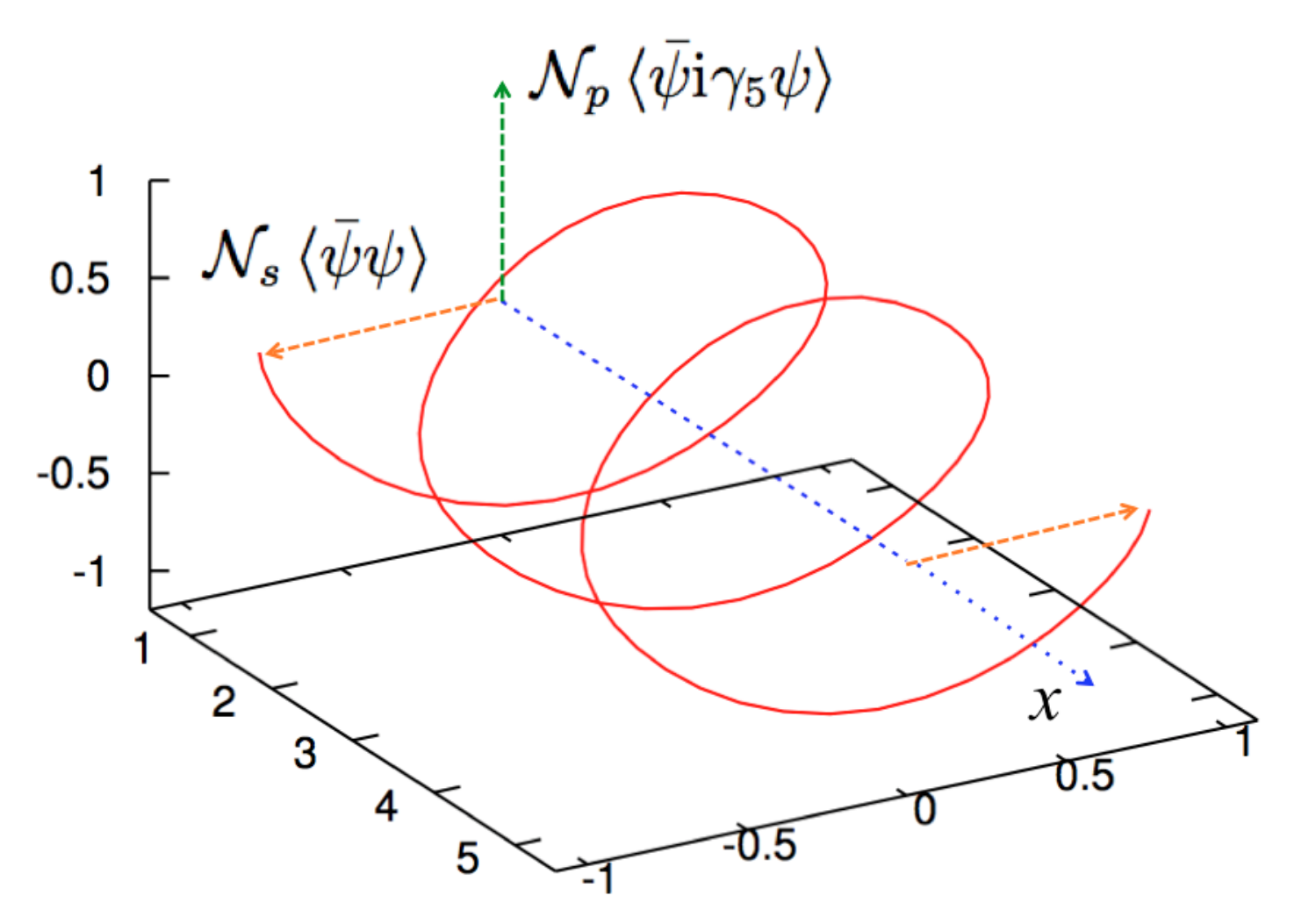
Figure 4: Left: The “elliptic” chiral spirals at λ=0.9\lambda=0.9. We plot the amplitude-free parts of condensates, 𝒩s​⟨ψ¯​ψ⟩≡⟨ψ¯​ψ⟩×G/N​𝒜=−ℳ\mathcal{N}_{s}\langle\bar{\psi}\psi\rangle\equiv\langle\bar{\psi}\psi\rangle\times G/N\mathcal{A}=-\mathcal{M} and 𝒩p​⟨ψ¯​i​γ5​ψ⟩≡⟨ψ¯​i​γ5​ψ⟩×2​π/N​𝐊′​𝒜=∂ξℳ\mathcal{N}_{p}\langle\bar{\psi}\mathrm{i}\gamma_{5}\psi\rangle\equiv\langle\bar{\psi}\mathrm{i}\gamma_{5}\psi\rangle\times 2\pi/N{\bf K}^{\prime}\mathcal{A}=\partial_{\xi}\mathcal{M}. Right: The plots at λ=0.9\lambda=0.9 for the (normalized) scalar (S), pseudoscalar (PS), and fermion number density (n). For the fermion number density, we divide by N​pF/πNp_{F}/\pi. The fermion number is stuck at the location of the domain wall where the scalar density passes zero.

We consider the high and low density limits and examine qualitative aspects of the quantities which we have computed so far. To begin with, we first express λ\lambda in terms of pF/M0p_{F}/M_{0}. The transcendental equation (68) in the λ→0\lambda\rightarrow 0 and λ→1\lambda\rightarrow 1 cases becomes

π​M0 2​pF=λ𝐊(λ)→{λ​π2​[ 1+λ4+O⁡(λ2)](λ→0)1 2​ln⁡ 16λ1+O⁡(λ1​ln⁡λ1)(λ→1),\frac{\,\pi M_{0}\,}{\,2p_{F}\,}=\sqrt{\lambda}\,{\bf K}(\lambda)~\rightarrow~\left\{\begin{matrix}~~~\frac{\,\sqrt{\lambda}\,\pi}{2}\left[\,1+\frac{\lambda}{4}+O(\lambda^{2})\,\right]~~~~~~~&(\lambda\rightarrow 0)\\ ~~~\frac{1}{\,2\,}\ln\frac{\,16\,}{\,\lambda_{1}\,}+O(\lambda_{1}\ln\lambda_{1})~~~~~~&(\lambda\rightarrow 1)\end{matrix}\right.\,, (80)

from which we get

λ={(M0pF)2− 1 2​(M0pF)4+O⁡(M06/pF6)(M0/pF≪1)1−16e−πM0/pF+O(e−2πM0/pF)(1≪M0/pF).\lambda=\left\{\begin{matrix}~~~\left(\frac{\,M_{0}\,}{\,p_{F}\,}\right)^{2}-\frac{\,1\,}{\,2\,}\left(\frac{\,M_{0}\,}{\,p_{F}\,}\right)^{4}+O(M_{0}^{6}/p_{F}^{6})~~~~~~~&(M_{0}/p_{F}\ll 1)\\ ~~~~1-16\,\mathrm{e}^{-\pi M_{0}/p_{F}}+O\left(\mathrm{e}^{-2\pi M_{0}/p_{F}}\right)~~~~~~~&(1\ll M_{0}/p_{F})\end{matrix}\right.\,. (81)

Next, we look at the parameter 𝒜\mathcal{A} which appears in place of the coordinate, ξ=𝒜​x\xi=\mathcal{A}x. Its asymptotic behavior is given by

𝒜= 2​𝐊​(λ)πpF={pF​[ 1+1 4​(M0pF)2+O⁡(M04/pF4)](M0/pF≪1)M0+O(pFe−πM0/pF)(1≪M0/pF).\mathcal{A}=\frac{\,2{\bf K}(\lambda)\,}{\pi}p_{F}=\left\{\begin{matrix}~~~p_{F}\left[\,1+\frac{1}{\,4\,}\left(\frac{\,M_{0}\,}{\,p_{F}\,}\right)^{2}+O(M_{0}^{4}/p_{F}^{4})\,\right]~~~~~~~&(M_{0}/p_{F}\ll 1)\\ ~~M_{0}\,+\,O\left(p_{F}\,\mathrm{e}^{-\pi M_{0}/p_{F}}\right)~~~~~~~~~&(1\ll M_{0}/p_{F})\end{matrix}\right.\,. (82)

Now we shall consider the physical quantities of particular interest.

(i) The asymptotic behavior of the energy gap is

Δg≡ωF′−ωF=(1−λ1)𝒜={M0×M0 2​pF+⋯(M0/pF≪1)M0+⋯(1≪M0/pF).\Delta_{g}\equiv\omega_{F}^{\prime}-\omega_{F}=\left(1-\sqrt{\lambda_{1}}\right)\mathcal{A}=\left\{\begin{matrix}~~M_{0}\times\frac{\,M_{0}\,}{\,2p_{F}\,}+\cdots~~~~~&(M_{0}/p_{F}\ll 1)\\ ~~M_{0}+\cdots~~~~&(1\ll M_{0}/p_{F})\end{matrix}\right.\,. (83)

In particular, at high density the gap is proportional to 1/pF1/p_{F} and tends to close rather quickly. It is important to notice that this quick decreasing behavior is not generic in other two-dimensional models. For instance, in the NJL2 model the gap stays at the vacuum value, ∼M0\sim M_{0}. We will discuss this issue more in Sec.IV.

(ii) The low density behaviors of the chiral scalar and pseudoscalar condensates are

⟨ψ¯​ψ⟩N≃−M0G​tanh⁡(M0​x),⟨ψ¯​i​γ5​ψ⟩N≃M04​1cosh2⁡(M0​x).(1≪M0/pF)\frac{\,\langle\bar{\psi}\psi\rangle\,}{N}\simeq-\,\frac{\,M_{0}\,}{G}\tanh(M_{0}x)\,,~~~~~\frac{\,\langle\bar{\psi}\mathrm{i}\gamma_{5}\psi\rangle\,}{N}\simeq\,\frac{\,M_{0}\,}{4}\frac{1}{\,\cosh^{2}(M_{0}x)\,}\,.~~~(1\ll M_{0}/p_{F}) (84)

This is the solution for widely separated kinks. When the scalar density becomes zero, the pseudoscalar density is maximized. On the other hand, the scalar density is maximized when the pseudoscalar density is zero. Therefore, the combination of the scalar and pseudoscalar density forms the chiral spirals, as shown in Fig.4.

(iii) The high density behaviors of the chiral scalar and pseudoscalar condensates are

⟨ψ¯​ψ⟩N≃−ΔgGΛsin(2pFx),⟨ψ¯​i​γ5​ψ⟩N≃ΔgG2​pFcos(2pFx),(M0/pF≪1)\frac{\,\langle\bar{\psi}\psi\rangle\,}{N}\simeq-\,\frac{\,\Delta_{g}\,}{\,G_{\Lambda}\,}\sin(2p_{F}x)\,,~~~~~\frac{\,\langle\bar{\psi}\mathrm{i}\gamma_{5}\psi\rangle\,}{N}\simeq\frac{\,\Delta_{g}\,}{\,G_{2p_{F}}\,}\cos(2p_{F}x)\,,~~~(M_{0}/p_{F}\ll 1) (85)

where G2​pFG_{2p_{F}} is defined by substituting 2​pF2p_{F} in place of Λ\Lambda in the coupling constant G⁡(Λ)G(\Lambda). This disparity of the effective coupling constants reflects the fact that the scalar and pseudoscalar density acquire contributions from different domains. We can construct an approximate invariant,

(GΛ​⟨ψ¯​ψ⟩)2+(G2​pF​⟨ψ¯​i​γ5​ψ⟩)2≃N2​Δg2.\left(G_{\Lambda}\left\langle\bar{\psi}\psi\right\rangle\right)^{2}+\left(G_{2p_{F}}\left\langle\bar{\psi}\mathrm{i}\gamma_{5}\psi\right\rangle\right)^{2}\simeq N^{2}\Delta_{g}^{2}\,. (86)

As pFp_{F} becomes larger, the expression approaches the chiral spirals with equal amplitudes for the scalar and pseudoscalar density.

IV Discussions

Refer to caption
Refer to caption
Figure 5: The quasimomentum-energy dispersion. Left: For the GN model. The spectra contain the gapped region in the Fermi and Dirac sea. The size of the gap decreases like ∼M0×M0/pF\sim M_{0}\times M_{0}/p_{F} as pFp_{F} becomes large. Right: For the NJL2-type models. The gaps open only at the Fermi points. The size of the gap is known to be ∼M0\sim M_{0}, independently of the value of pFp_{F}.

In this section we examine the qualitative differences between the chiral spirals in the GN model and in the QCD2 or NJL2 models. First, we compare results of the GN model and of QCD2 by contrasting the short- and long-range interactions. Secondly, we argue why results of the GN and NJL2 models are qualitatively different, by emphasizing the structure of the 4-Fermi interactions.

IV.1 Short-range versus long-range interactions

First let us recall the structure of the single-particle energy levels in the GN model. The energy level has gaps in the Fermi and Dirac seas; see Fig. 5. In the chiral scalar density, contributions from the first energy branch in the Fermi and Dirac sea cancel out, leaving only the contribution from the second energy branch in the Dirac sea [see Eq. (70)],

⟨ψ¯​ψ⟩IFermi+(⟨ψ¯​ψ⟩I+⟨ψ¯​ψ⟩II)Dirac=⟨ψ¯​ψ⟩IIDirac.(GN​model)\langle\bar{\psi}\psi\rangle_{{\rm I}}^{{\rm Fermi}}+\left(\,\langle\bar{\psi}\psi\rangle_{{\rm I}}+\langle\bar{\psi}\psi\rangle_{{\rm II}}\,\right)^{{\rm Dirac}}=\langle\bar{\psi}\psi\rangle_{{\rm II}}^{{\rm Dirac}}\,.~~~~~~({\rm GN~model}) (87)

The condensate includes the contributions up to ω∼−Λ\omega\sim-\Lambda. This is the reason why the scalar density is proportional to ∼ln⁡(2​Λ/M0)\sim\ln(2\Lambda/M_{0}).

On the other hand, in the chiral pseudoscalar density, the Dirac sea contributions from the first and second energy branches cancel, leaving only the Fermi sea contribution,

⟨ψ¯​i​γ5​ψ⟩IFermi+(⟨ψ¯​i​γ5​ψ⟩I+⟨ψ¯​i​γ5​ψ⟩II)Dirac=⟨ψ¯​i​γ5​ψ⟩IFermi(GN​model).\langle\bar{\psi}\mathrm{i}\gamma_{5}\psi\rangle_{{\rm I}}^{{\rm Fermi}}+\left(\,\langle\bar{\psi}\mathrm{i}\gamma_{5}\psi\rangle_{{\rm I}}+\langle\bar{\psi}\mathrm{i}\gamma_{5}\psi\rangle_{{\rm II}}\,\right)^{{\rm Dirac}}=\langle\bar{\psi}\mathrm{i}\gamma_{5}\psi\rangle_{{\rm I}}^{{\rm Fermi}}~~~~({\rm GN~model})\,. (88)

The amplitude is proportional to ∼ln⁡(4​pF/M0)\sim\ln(4p_{F}/M_{0}). Due to the mismatch in the net contributions for the scalar and pseudoscalar density, their amplitudes are naturally different in the GN model.

When using this result as a guide for the QCD phase diagram, espcially when pFp_{F} becomes larger than the vacuum quark effective mass, we should use the GN results with some caution. The above result strongly depends on the fact that the gaps in the Fermi and Dirac sea have the same size at the edge of the first energy branches. Such large gaps in the Dirac sea are rather specific to models with the contact interactions. In such models, although the condensation is initially driven by the low-energy particle-hole pairs near the Fermi surface, the created condensate affects spectra all the way from the Fermi surface down to the Dirac sea. Then the resulting gapped fermions in the Dirac sea also contribute to the condensate, giving large feedback to the fermions near the Fermi surface. Therefore there is a tight connection between the structures of the Fermi sea and Dirac sea.

In contrast, for models of the long-range interactions such as QCD, the physics near the Fermi surface does not strongly affect the structure of the Dirac sea. In fact, with momentum-dependent forces, the gap functions in general become momentum dependent. If we had used models of long-range interactions such as 1/p→21/\vec{p}^{2} force, the gap would be large near the Fermi surface but small otherwise. In particular, the chirality-violating effective mass tends to disappear in the Dirac sea as fermion density becomes large [6]. Then the main contribution to both chiral scalar and pseudoscalar density comes from the Fermi sea, and they tend to acquire the same amplitude. Actually, this is what happens in models like QCD2.

IV.2 The GN model versus the NJL2 model

In the NJL2 model, the interaction is short range, as in the GN model. Nevertheless, qualtiative aspects of the chiral condensates are more similar to QCD2 rather than the GN model. Moreover, in contrast to the GN model, models in the latter class have an energy gap of ∼M0\sim M_{0} instead of a decreasing gap at finite density, ∼M02/pF\sim M_{0}^{2}/p_{F} (Fig. 5). The key observation to understanding all these tendencies is that for a particular set of 4-Fermi interactions, physics near the Fermi surface tends to decouple from physics in the Dirac sea, as it happens for models with long-range interactions.

To explain this, first we project the fermion fields onto the right- and left-moving components,

ψr,l= 1±γ0​γz2​ψ,γ5=γ0​γz.\psi_{r,\,l}=\frac{\,1\pm\gamma_{0}\gamma_{z}\,}{2}\psi\,,~~~~~~\gamma_{5}=\gamma_{0}\gamma_{z}\,. (89)

For free fermions, the field equation is given by

(p0−pz)​ψr=0,(p0+pz)​ψl=0,(p_{0}-p_{z})\psi_{r}=0\,,~~~~~~~(p_{0}+p_{z})\psi_{l}=0\,, (90)

from which we observe that the right components have positive energy for pz>0p_{z}>0 and negative energy for pz<0p_{z}<0. The relation is opposite for the left components.

Now we express the 4-Fermi interactions in terms of left and right components. For bookkeeping purposes, let

Φ⁡(x)≡ψ¯l​ψr​(x),Φ∗​(x)≡ψ¯r​ψl​(x).\Phi(x)\equiv\bar{\psi}_{l}\psi_{r}(x)\,,~~~~~~~\Phi^{*}(x)\equiv\bar{\psi}_{r}\psi_{l}(x)\,. (91)

The Fourier transform of Φ\Phi is (∫x≡∫d2x,∫q≡∫d2​q(2​π)2)\left(\int_{x}\equiv\int\mathrm{d}^{2}x\,,\int_{q}\equiv\int\frac{\mathrm{d}^{2}q}{\,(2\pi)^{2}\,}\right)

Φ⁡(q)=∫δ​pψ¯l​(−q2+δ​p)​ψr​(q2+δ​p).\Phi(q)=\int_{\delta p}\bar{\psi}_{l}\left(-\frac{q}{2}+\delta p\right)\,\psi_{r}\left(\frac{q}{2}+\delta p\right)\,. (92)

Notice that for qz≃2​pFq_{z}\simeq 2p_{F}, both of the fields ψr\psi_{r} and ψl\psi_{l} at small δ​pz\delta p_{z} describe the fermion fields near the Fermi points. If qzq_{z} is very different from 2​pF2p_{F}, either of the fields ψl\psi_{l} or ψr\psi_{r} in Φ⁡(q)\Phi(q) must be in the region far away from the Fermi surface, costing more energy. This is the reason why the homogeneous condensation at qz=0q_{z}=0 tends to disappear at finite density while instead the inhomogeneous condensate of ⟨Φ⁡(qz=2​pF)⟩\langle\Phi(q_{z}=2p_{F})\rangle develops due to the condensed particle-hole pairs near the Fermi surface.

Now we consider the 4-Fermi interaction in the NJL2. It can be written as

∫x[(ψ¯​ψ)2+(ψ¯​i​γ5​ψ)2]=4​∫x|Φ⁡(x)|2=4​∫qΦ⁡(q)​Φ∗​(q),\int_{x}\left[(\bar{\psi}\psi)^{2}+(\bar{\psi}\mathrm{i}\gamma_{5}\psi)^{2}\right]=4\int_{x}|\Phi(x)|^{2}=4\int_{q}\Phi(q)\Phi^{*}(q)\,, (93)

Note that the interaction couples Φ⁡(q)\Phi(q) with Φ∗​(q)\Phi^{*}(q). When one Φ⁡(q)\Phi(q) is replaced with the mean field ⟨Φ⁡(qz=2​pF)⟩\langle\Phi(q_{z}=2p_{F})\rangle, it affects only Φ∗​(qz=2​pF)\Phi^{*}(q_{z}=2p_{F}) in which left- and right-moving fermions can simultaneously stay at low energy for small δ​pz\delta p_{z}, and also simultaneously go to high energy for large δ​pz\delta p_{z}. Phrasing this in another way, the mean field scatters low-energy fields to low energy, and high-energy fields to high energy, but it does not strongly mix up fields belonging to different energy domains.

The meaning of the above statements becomes clearer if we consider the GN model. Its 4-Fermi interaction is

∫x(ψ¯​ψ)2=∫x[ 2​|Φ⁡(x)|2+Φ2+Φ∗2]=∫q[ 2​Φ​(q)​Φ∗​(q)+Φ⁡(q)​Φ​(−q)+Φ∗​(q)​Φ∗​(−q)],\int_{x}(\bar{\psi}\psi)^{2}=\!\int_{x}\!\left[\,2|\Phi(x)|^{2}+\Phi^{2}+\Phi^{*2}\right]=\!\int_{q}\left[\,2\Phi(q)\Phi^{*}(q)+\Phi(q)\Phi(-q)+\Phi^{*}(q)\Phi^{*}(-q)\right]\,, (94)

where we find extra couplings, Φ⁡(q)​Φ​(−q)\Phi(q)\Phi(-q) and Φ∗​(q)​Φ∗​(−q)\Phi^{*}(q)\Phi^{*}(-q). Now imagine that we have a mean field, ⟨Φ⁡(qz=2​pF)⟩\langle\Phi(q_{z}=2p_{F})\rangle. Then it couples to the composite field Φ⁡(qz=−2​pF)\Phi(q_{z}=-2p_{F}). But its content is

Φ⁡(qz=−2​pF)=∫δ​pψ¯l​(pF+δ​p)​ψr​(−pF+δ​p).\Phi(q_{z}=-2p_{F})=\int_{\delta p}\bar{\psi}_{l}\left(p_{F}+\delta p\right)\,\psi_{r}\left(-p_{F}+\delta p\right)\,. (95)

At small δ​pz\delta p_{z}, both fields are in the Dirac sea according to the dispersion (90). On the other hand, when the right field ψr\psi_{r} stays near the Fermi surface, then δ​pz≃2​pF\delta p_{z}\simeq 2p_{F}, and the ψl\psi_{l} field is in the Dirac sea with energy of ∼−3​pF\sim-3p_{F}. Therefore, if the mean field is developed by condensation near the Fermi surface, it inevitably couples the fields near the Fermi surface to those in the Dirac sea. This is the reason why the GN model has the sizable energy gap not only near the Fermi surface but also in the Dirac sea. Furthermore, the feedback from the Dirac sea condensation strongly affects the Fermi surface condensations, making the inhomogeneous solutions far more complicated than those in the NJL2 model. Because of this feedback, the size of the mass gap in the GN model scales like ∼M02/pF\sim M_{0}^{2}/p_{F}, unlike ∼M0\sim M_{0} in the NJL2 model or QCD2.

Perhaps it is already clear why the results of chiral condensates in NJL2 and QCD2 are similar. In the former, the combinations of the 4-Fermi interactions are arranged in such a way that fields for the Fermi surface do not strongly couple to those for the Dirac sea. In the latter, the long-range interactions and the resulting momentum-dependent mass functions tend to forbid strong coupling between the Fermi surface and Dirac sea. In both cases, physics are governed by dynamics near the Fermi surface.

V Summary

In this paper, we have argued that the inhomogeneous chiral condensate in the GN model takes the chiral spiral form. Although the thermodynamic functional does not depend on the pseudoscalar density manifestly, the spatial modulations of the chiral scalar density inevitably generate the pseudoscalar density modulations.

While our arguments add little for the understanding of the GN model, the implications will become important once we start to infer proper effective models at finite quark density from more general perspectives on the fundamental theories. For assumed mean fields, we should calculate not only the thermodynamic functional but also various operators which might acquire large expectation values. Once such operators are found, we have to reanalyze the effective models including the interaction terms related to such operators, unless there is some reason to discard them. For the NJL4 up to dimensions-6 operators, it is perhaps unavoidable to add (ψ¯​i​γ0​γj​ψ)2(\bar{\psi}\mathrm{i}\gamma_{0}\gamma_{j}\psi)^{2}-type 4-Fermi interactions whose two-dimensional counterpart is (ψ¯​i​γ5​ψ)2​D2(\bar{\psi}\mathrm{i}\gamma_{5}\psi)_{{\rm 2D}}^{2}. This is an approach pursued in Ref. [11].

We have also contrasted the GN model with the NJL2 model and QCD2 to understand the structure of the chiral spirals and the parametric behaviors of the mass gaps. In the GN model, the specific form of the 4-Fermi interaction and its short-range properties together create a strong Fermi-Dirac sea coupling which deforms the Dirac sea, even producing the energy gap inside the Dirac sea. If the interaction is replaced with the long-range one, such strong deformation of the Dirac sea tends to disappear. Similar results can be found if we arrange the 4-Fermi interactions in such a way as to weaken couplings between the Fermi and Dirac seas, as happened in the NJL2 model.

We found it very interesting that simple arrangements of the 4-Fermi interactions can control the coupling between the Fermi and Dirac sea contributions. Even within models with contact interactions, we can reproduce results similar to those in models with long-range interactions. Perhaps we may use the above kinematic considerations as a guide to restrict possible forms of the effective models at finite density, in addition to the ordinary symmetry considerations.

More implications from the GN model studies to the results of the NJL4 model will be discussed elsewhere.

Acknowledgments

T.K. acknowledges E. J. Ferrer, V. de la Incera, and S. Carignano for very stimulating discussions which motivate this work and for their kind hospitality during his visit to UTEP. This research was supported in part by NSF Grants No. PHY09-69790 and No. PHY13-05891.

Appendix A Series expansion of the elliptic functions

The series expansion for the elliptic functions is useful for several purposes, such as numerical computations. We have already given the expansion for Jacobi’s θ\theta function and ZZ function in Eqs. (26) and (28). The expansions for the elliptic functions are (q≡e−π𝐊′/𝐊q\equiv\mathrm{e}^{-\pi{\bf K}^{\prime}/{\bf K}}) 1111 11 Formula (16.23) in Ref. [12].

sn⁡(x|λ)\displaystyle\mathrm{sn}(x|\lambda) =2​πλ1/2​𝐊​∑n=0qn+1/2 1−q2​n+1​sin⁡(2​n+1)​π​x2​𝐊,\displaystyle=\frac{2\pi}{\lambda^{1/2}{\bf K}}\sum_{n=0}\frac{q^{n+1/2}}{\,1-q^{2n+1}\,}\sin\frac{\,(2n+1)\pi x\,}{2{\bf K}}\,,
cn⁡(x|λ)\displaystyle\mathrm{cn}(x|\lambda) =2​πλ1/2​𝐊​∑n=0qn+1/2 1+q2​n+1​cos⁡(2​n+1)​π​x2​𝐊,\displaystyle=\frac{2\pi}{\,\lambda^{1/2}{\bf K}\,}\sum_{n=0}\frac{q^{n+1/2}}{\,1+q^{2n+1}\,}\cos\frac{\,(2n+1)\pi x\,}{2{\bf K}}\,,
dn⁡(x|λ)\displaystyle\mathrm{dn}(x|\lambda) =−π 2​𝐊+2​π𝐊​∑n=0qn 1+q2​n​cos⁡n​π​x𝐊.\displaystyle=-\frac{\pi}{\,2{\bf K}\,}+\frac{2\pi}{\,{\bf K}\,}\sum_{n=0}\frac{q^{n}}{\,1+q^{2n}\,}\cos\frac{\,n\pi x\,}{{\bf K}}\,. (96)

For small λ\lambda, the elliptic functions can be expanded as 1212 12 Formula (16.22) in Ref. [12].

sn⁡(x|λ)=x−(1+λ)​x33!+⋯,cn⁡(x|λ)=1−x22!+⋯,dn⁡(x|λ)=1−λ​x22!+⋯.\mathrm{sn}(x|\lambda)=x-(1+\lambda)\frac{\,x^{3}\,}{3!}+\cdots\,,~~~\mathrm{cn}(x|\lambda)=1-\frac{\,x^{2}\,}{2!}+\cdots\,,~~~\mathrm{dn}(x|\lambda)=1-\lambda\frac{\,x^{2}\,}{2!}+\cdots\,. (97)

Appendix B Relative phases

To determine χ~\tilde{\chi} from φ~\tilde{\varphi} including the relative phase, we use Eqs.(6) and (35). We first compute the derivative. First we note that

d​φ~d​ξ=[π 2​𝐊​(1θ1​(uξ+α)​d​θ1​(uξ+α)d​uξ+α−1θ4​(uξ)​d​θ4​(uξ)d​uξ)−Z⁡(α)]​φ~​(ξ).\frac{\mathrm{d}\tilde{\varphi}}{\mathrm{d}\xi}=\left[\,\frac{\,\pi\,}{\,2{\bf K}\,}\left(\frac{1}{\,\theta_{1}(u_{\xi+\alpha})\,}\frac{\,\mathrm{d}\theta_{1}(u_{\xi+\alpha})\,}{\mathrm{d}u_{\xi+\alpha}}-\frac{1}{\,\theta_{4}(u_{\xi})\,}\frac{\,\mathrm{d}\theta_{4}(u_{\xi})\,}{\mathrm{d}u_{\xi}}\right)-Z(\alpha)\,\right]\tilde{\varphi}(\xi)\,. (98)

To proceed further, we need to use the formulas 1313 13 Formula (16.34) in Ref. [12]..

1θ1​(ua)​d​θ1​(ua)d​ua= 2​𝐊π​[Z⁡(a)+cn⁡(a)​dn​(a)sn⁡(a)],1θ4​(ua)​d​θ4​(ua)d​ua= 2​𝐊π​Z​(a),\frac{1}{\,\theta_{1}(u_{a})\,}\frac{\,\mathrm{d}\theta_{1}(u_{a})\,}{\mathrm{d}u_{a}}=\frac{\,2{\bf K}\,}{\pi}\left[\,Z(a)+\frac{\,\mathrm{cn}(a)\,\mathrm{dn}(a)\,}{\mathrm{sn}(a)}\right]\,,~~~~~~~\frac{1}{\,\theta_{4}(u_{a})\,}\frac{\,\mathrm{d}\theta_{4}(u_{a})\,}{\mathrm{d}u_{a}}=\frac{\,2{\bf K}\,}{\pi}\,Z(a)\,, (99)

with which we get

d​φ~d​ξ=[Z⁡(ξ+α)+cn⁡(ξ+α)​dn​(ξ+α)sn⁡(ξ+α)−Z⁡(ξ)−Z⁡(α)]​φ~​(ξ).\frac{\,\mathrm{d}\tilde{\varphi}\,}{\mathrm{d}\xi}=\left[\,Z(\xi+\alpha)+\frac{\,\mathrm{cn}(\xi+\alpha)\,\mathrm{dn}(\xi+\alpha)\,}{\mathrm{sn}(\xi+\alpha)}-Z(\xi)-Z(\alpha)\,\right]\tilde{\varphi}(\xi)\,. (100)

Next we use the addition theorem for the zeta function 1414 14 Formula (17.4.35) in Ref. [12].,

Z⁡(ξ+α)=Z⁡(ξ)+Z⁡(α)−λ​sn​(ξ)​sn​(α)​sn​(ξ+α),Z(\xi+\alpha)=Z(\xi)+Z(\alpha)-\lambda\,\mathrm{sn}(\xi)\,\mathrm{sn}(\alpha)\,\mathrm{sn}(\xi+\alpha)\,, (101)

and for the elliptic functions 1515 15 Formula (16.17) in Ref. [12].,

sn⁡(u+v)\displaystyle\mathrm{sn}(u+v) =sn⁡(u)⋅cn⁡(v)​dn​(v)+sn⁡(v)⋅cn⁡(u)​dn​(u)1−λ​sn2​(u)⋅sn2​(v),\displaystyle=\frac{\,\mathrm{sn}(u)\cdot\mathrm{cn}(v)\mathrm{dn}(v)+\mathrm{sn}(v)\cdot\mathrm{cn}(u)\mathrm{dn}(u)\,}{1-\lambda\,\mathrm{sn}^{2}(u)\cdot\mathrm{sn}^{2}(v)}\,,
cn⁡(u+v)\displaystyle\mathrm{cn}(u+v) =cn⁡(u)⋅cn⁡(v)−sn⁡(u)​dn​(u)⋅sn⁡(v)​dn​(v)1−λ​sn2​(u)⋅sn2​(v),\displaystyle=\frac{\,\mathrm{cn}(u)\cdot\mathrm{cn}(v)-\mathrm{sn}(u)\mathrm{dn}(u)\cdot\mathrm{sn}(v)\mathrm{dn}(v)\,}{1-\lambda\,\mathrm{sn}^{2}(u)\cdot\mathrm{sn}^{2}(v)}\,,
dn⁡(u+v)\displaystyle\mathrm{dn}(u+v) =dn⁡(u)⋅dn⁡(v)−λ​sn​(u)​cn​(u)⋅sn⁡(v)​cn​(v)1−λ​sn2​(u)⋅sn2​(v).\displaystyle=\frac{\,\mathrm{dn}(u)\cdot\mathrm{dn}(v)-\lambda\,\mathrm{sn}(u)\mathrm{cn}(u)\cdot\mathrm{sn}(v)\mathrm{cn}(v)\,}{1-\lambda\,\mathrm{sn}^{2}(u)\cdot\mathrm{sn}^{2}(v)}\,. (102)

With these ingredients, we have to do messy calculations and get

χ~ω​(ξ)=−sgn⁡(ω~)​ 1dn⁡(ξ)​cn⁡(ξ+α)sn⁡(ξ+α)​φ~ω​(ξ).\tilde{\chi}_{\omega}(\xi)=-{\rm sgn}(\tilde{\omega})\frac{\,1\,}{\,\mathrm{dn}(\xi)\,}\,\frac{\,\mathrm{cn}(\xi+\alpha)\,}{\,\mathrm{sn}(\xi+\alpha)\,}\,\tilde{\varphi}_{\omega}(\xi)\,. (103)

In the final step we use the relations among the theta functions and elliptic functions [Sec.(22.11) in Ref. [13]],

sn⁡(a)=θ3​(0)θ2​(0)​θ1​(ua)θ4​(ua),cn⁡(a)=θ4​(0)θ2​(0)​θ2​(ua)θ4​(ua),dn⁡(a)=θ4​(0)θ3​(0)​θ3​(ua)θ4​(ua),\mathrm{sn}(a)=\frac{\,\theta_{3}(0)\,}{\theta_{2}(0)}\,\frac{\,\theta_{1}(u_{a})\,}{\theta_{4}(u_{a})}\,,~~~~~\mathrm{cn}(a)=\frac{\,\theta_{4}(0)\,}{\theta_{2}(0)}\,\frac{\,\theta_{2}(u_{a})\,}{\theta_{4}(u_{a})}\,,~~~~~\mathrm{dn}(a)=\frac{\,\theta_{4}(0)\,}{\theta_{3}(0)}\,\frac{\,\theta_{3}(u_{a})\,}{\theta_{4}(u_{a})}\,, (104)

and then use the expression for φ~​(ξ)\tilde{\varphi}(\xi). The result is

χ~ω​(ξ)=−sgn⁡(ω~)​θ2​(uξ+α)θ3​(uξ)​θ4​(uξ)θ1​(uξ+α)​φ~ω​(ξ)=−𝒩​sgn​(ω~)​θ2​(uξ+α)θ3​(uξ)​eξ​Z​(α).\tilde{\chi}_{\omega}(\xi)=-{\rm sgn}(\tilde{\omega})\,\frac{\,\theta_{2}(u_{\xi+\alpha})\,}{\,\theta_{3}(u_{\xi})\,}\,\frac{\,\theta_{4}(u_{\xi})\,}{\,\theta_{1}(u_{\xi+\alpha})\,}\,\tilde{\varphi}_{\omega}(\xi)=-\mathcal{N}{\rm sgn}(\tilde{\omega})\,\frac{\,\theta_{2}(u_{\xi+\alpha})\,}{\,\theta_{3}(u_{\xi})\,}\,\mathrm{e}^{\xi Z(\alpha)}\,. (105)

This expression can be converted into a more convenient form. To do this, we note that by definition the functions θ2\theta_{2} and θ3\theta_{3} are related to θ1\theta_{1} and θ4\theta_{4} as

θ2​(u)=θ1​(u+u𝐊)=−θ1​(u−u𝐊),θ3​(u)=θ4​(u+u𝐊)=θ4​(u−u𝐊),\theta_{2}(u)=\theta_{1}(u+u_{\bf K})=-\theta_{1}(u-u_{\bf K})\,,~~~~~\theta_{3}(u)=\theta_{4}(u+u_{\bf K})=\theta_{4}(u-u_{\bf K})\,, (106)

so the function χ~​(ξ)\tilde{\chi}(\xi) is proportional to φ~​(ξ−𝐊)\tilde{\varphi}(\xi-{\bf K}),

χ~ω​(ξ)=sgn⁡(ω~)​e𝐊​Z​(α)×𝒩​θ1​(uξ−𝐊+α)θ4​(uξ−𝐊)​e(ξ−𝐊)​Z​(α)=sgn⁡(ω~)​e𝐊​Z​(α)×φ~ω​(ξ−𝐊),\tilde{\chi}_{\omega}(\xi)={\rm sgn}(\tilde{\omega})\,\mathrm{e}^{{\bf K}Z(\alpha)}\times\mathcal{N}\frac{\,\theta_{1}(u_{\xi-{\bf K}+\alpha})\,}{\,\theta_{4}(u_{\xi-{\bf K}})\,}\,\mathrm{e}^{(\xi-{\bf K})Z(\alpha)}={\rm sgn}(\tilde{\omega})\,\mathrm{e}^{{\bf K}Z(\alpha)}\times\tilde{\varphi}_{\omega}(\xi-{\bf K})\,, (107)

as it should be. Note that the exponent is purely imaginary.

Appendix C Normalization factor

The equation to determine the normalization factor is

1 2=1 2​𝐊​∫02​𝐊d​ξ​|φ~ω​(ξ)|2=|𝒩ω|2 2​𝐊​∫02​𝐊d​ξ​θ1​(uξ+α)​θ1​(uξ+α∗)θ42​(uξ),\frac{1}{\,2\,}=\frac{1}{\,2{\bf K}\,}\int_{0}^{2{\bf K}}\!\mathrm{d}\xi\,|\tilde{\varphi}_{\omega}(\xi)|^{2}=\frac{\,|\mathcal{N}_{\omega}|^{2}\,}{\,2{\bf K}\,}\int_{0}^{2{\bf K}}\!\mathrm{d}\xi\,\frac{\,\theta_{1}(u_{\xi+\alpha})\theta_{1}(u_{\xi+\alpha^{*}})\,}{\,\theta^{2}_{4}(u_{\xi})\,}\,, (108)

for each energy ω\omega. We use the formula

θ32​(0)​θ1​(a+b)​θ1​(a−b)=θ42​(a)​θ22​(b)−θ42​(b)​θ22​(a).\theta^{2}_{3}(0)\theta_{1}(a+b)\theta_{1}(a-b)=\theta_{4}^{2}(a)\theta_{2}^{2}(b)-\theta_{4}^{2}(b)\theta_{2}^{2}(a)\,. (109)

Similar formulas and derivations can be found in Chap. 21 in Ref. [13].

(i) The α=i​η\alpha=\mathrm{i}\eta case. In this case, α∗=−α\alpha^{*}=-\alpha, and we get

θ1​(uξ+α)​θ1​(uξ−α)θ42​(uξ)=θ22​(uα)θ32​(0)​[ 1−θ42​(uα)θ22​(uα)​θ22​(ξ)θ42​(ξ)]=θ22​(uα)θ32​(0)​[ 1−cn2​(ξ)cn2​(α)],\frac{\,\theta_{1}(u_{\xi+\alpha})\theta_{1}(u_{\xi-\alpha})\,}{\,\theta^{2}_{4}(u_{\xi})\,}=\frac{\,\theta_{2}^{2}(u_{\alpha})\,}{\,\theta_{3}^{2}(0)\,}\left[\,1-\frac{\,\theta_{4}^{2}(u_{\alpha})\,}{\,\theta_{2}^{2}(u_{\alpha})\,}\frac{\,\theta_{2}^{2}(\xi)\,}{\,\theta_{4}^{2}(\xi)\,}\,\right]=\frac{\,\theta_{2}^{2}(u_{\alpha})\,}{\,\theta_{3}^{2}(0)\,}\left[\,1-\frac{\,\mathrm{cn}^{2}(\xi)\,}{\,\mathrm{cn}^{2}(\alpha)\,}\,\right]\,, (110)

where we have used Eq.(104). Finally, we take the spatial integral. Recalling Eq.(39), we find

|𝒩ω|−2=2λ​cn2​(α)​θ22​(uα)θ32​(0)​[dn2​(α)−𝐄𝐊].|\mathcal{N}_{\omega}|^{-2}=\frac{2}{\,\lambda\mathrm{cn}^{2}(\alpha)\,}\frac{\,\theta_{2}^{2}(u_{\alpha})\,}{\,\theta_{3}^{2}(0)\,}\left[\,\mathrm{dn}^{2}(\alpha)-\frac{\,{\bf E}\,}{\,{\bf K}\,}\,\right]\,. (111)

Combining Eqs.(110) and (111), we can arrive at the expression (38).

(ii) The α=𝐊+i​η\alpha={\bf K}+\mathrm{i}\eta case. We recall the relation (27), θ1​(uξ+2​𝐊)=−θ1​(uξ)\theta_{1}(u_{\xi+2{\bf K}})=-\theta_{1}(u_{\xi}). Then

θ1​(uξ+𝐊+i​η)​θ1​(uξ+𝐊−i​η)=−θ1​(uξ+𝐊+i​η)​θ1​(uξ−𝐊−i​η),\theta_{1}(u_{\xi+{\bf K}+\mathrm{i}\eta})\theta_{1}(u_{\xi+{\bf K}-\mathrm{i}\eta})=-\theta_{1}(u_{\xi+{\bf K}+\mathrm{i}\eta})\theta_{1}(u_{\xi-{\bf K}-\mathrm{i}\eta})\,, (112)

so θ1​(uξ+α)​θ1​(uξ+α∗)=−θ1​(uξ+α)​θ1​(uξ−α)\theta_{1}(u_{\xi+\alpha})\theta_{1}(u_{\xi+\alpha^{*}})=-\theta_{1}(u_{\xi+\alpha})\theta_{1}(u_{\xi-\alpha}). Therefore we can obtain results corresponding to Eqs.(110) and (111) by multiplying them by (−1)(-1). On the other hand, the (−1)(-1) factors will cancel for the normalized probability function |φ~​(ξ)|2|\tilde{\varphi}(\xi)|^{2}, so Eq.(38) takes the same form for the α=i​η\alpha=\mathrm{i}\eta and 𝐊+i​η{\bf K}+\mathrm{i}\eta cases.

Appendix D Derivative of the Zeta-function

To compute the derivative of the zeta function, we use the expression 1616 16 Formula (17.4.28) in Ref. [12].

Z⁡(α)=E⁡(α)−α​𝐄/𝐊,Z(\alpha)=E(\alpha)-\alpha{\bf E}/{\bf K}\,, (113)

where E⁡(α)E(\alpha) is the Jacobi incomplete elliptic integral,

E⁡(α)=∫0αd​w​dn2​w.E(\alpha)=\int^{\alpha}_{0}\!\mathrm{d}w~\mathrm{dn}^{2}w\,. (114)

In particular, for α=𝐊\alpha={\bf K}, we have the complete integral, E⁡(𝐊)=𝐄E({\bf K})={\bf E}. From these expressions we can easily arrive at Eq.(42).

Appendix E More on the UV cutoff

Here we will complete the discussions outlined in Sec.II.4. First, we express ωΛ\omega_{\Lambda} by ϵ\epsilon. Using the Jacobi imaginary transformation and then applying the relation for the quarter period, we get [remember that 𝐊′​(λ)=𝐊⁡(λ1){\bf K}^{\prime}(\lambda)={\bf K}(\lambda_{1})]

ωΛ𝒜=dn⁡(i⁡(𝐊′−ϵ)|λ)=dn⁡(𝐊′−ϵ|λ1)cn⁡(𝐊′−ϵ|λ1)= 1sn⁡(ϵ|λ1).\frac{\,\omega_{\Lambda}\,}{\mathcal{A}}=\mathrm{dn}\left(\,\mathrm{i}({\bf K}^{\prime}-\epsilon)|\lambda\,\right)=\frac{\,\mathrm{dn}({\bf K}^{\prime}-\epsilon\,|\lambda_{1})\,}{\,\mathrm{cn}({\bf K}^{\prime}-\epsilon\,|\lambda_{1})\,}=\frac{\,1\,}{\,\mathrm{sn}(\epsilon\,|\lambda_{1})\,}\,. (115)

Then, expanding the elliptic functions via Eq.(97), we get

ωΛ𝒜=1ϵ​[ 1+(1+λ1)​ϵ23!+⋯].\frac{\,\omega_{\Lambda}\,}{\mathcal{A}}=\frac{1}{\,\epsilon\,}\left[\,1+(1+\lambda_{1})\,\frac{\,\epsilon^{2}\,}{3!}+\cdots\right]\,. (116)

Next, we treat our dispersion at quasimomenum Q=ΛQ=\Lambda,

Λ𝒜=−i​Z​(i⁡(𝐊′−ϵ)|λ)+π 2​𝐊.\frac{\,\Lambda\,}{\,\mathcal{A}\,}=-\mathrm{i}Z\left(\,\mathrm{i}({\bf K}^{\prime}-\epsilon)|\lambda\,\right)+\frac{\,\pi\,}{\,2{\bf K}\,}\,. (117)

Using the imaginary transformation formula 1717 17 Formula (17.4.36) in Ref. [12].,

i​Z​(i⁡(𝐊′−ϵ)|λ)=Z⁡(𝐊′−ϵ|λ1)−dn⁡(𝐊′−ϵ|λ1)​sn⁡(𝐊′−ϵ|λ1)cn⁡(𝐊′−ϵ|λ1)+π 2​𝐊​(1−ϵ𝐊′).\mathrm{i}Z\left(\,\mathrm{i}({\bf K}^{\prime}-\epsilon)|\lambda\,\right)=Z({\bf K}^{\prime}-\epsilon|\lambda_{1})-\mathrm{dn}({\bf K}^{\prime}-\epsilon|\lambda_{1})\,\frac{\,\mathrm{sn}({\bf K}^{\prime}-\epsilon|\lambda_{1})\,}{\,\mathrm{cn}({\bf K}^{\prime}-\epsilon|\lambda_{1})\,}+\frac{\pi}{\,2{\bf K}\,}\left(1-\frac{\epsilon}{{\bf K}^{\prime}}\right)\,. (118)

The computation of the first term on the rhs requires comment. Using Eq.(113) and then formulas 1818 18 Formulas (17.4.28) and (17.4.7) in Ref. [12]., we get

Z⁡(𝐊′−ϵ|λ1)\displaystyle Z({\bf K}^{\prime}-\epsilon|\lambda_{1}) =E⁡(𝐊′−ϵ|λ1)−𝐄′𝐊′​(𝐊′−ϵ)\displaystyle=E({\bf K}^{\prime}-\epsilon|\lambda_{1})-\frac{\,{\bf E}^{\prime}\,}{{\bf K}^{\prime}}\left({\bf K}^{\prime}-\epsilon\right)
=𝐄′−E⁡(ϵ|λ1)+λ1​sn⁡(ϵ|λ1)​cn​(ϵ|λ1)dn⁡(ϵ|λ1)−𝐄′𝐊′​(𝐊′−ϵ)\displaystyle={\bf E}^{\prime}-E(\epsilon|\lambda_{1})+\lambda_{1}\frac{\,\mathrm{sn}(\epsilon|\lambda_{1})\mathrm{cn}(\epsilon|\lambda_{1})\,}{\mathrm{dn}(\epsilon|\lambda_{1})}-\frac{\,{\bf E}^{\prime}\,}{{\bf K}^{\prime}}\left({\bf K}^{\prime}-\epsilon\right)
=−ϵ⁡(λ−𝐄′𝐊′)+O⁡(ϵ3).\displaystyle=-\epsilon\left(\lambda-\frac{\,{\bf E}^{\prime}\,}{{\bf K}^{\prime}}\right)+O(\epsilon^{3})\,. (119)

The remaining calculations are straightforward. We can express the momentum cutoff Λ\Lambda as a function of ϵ\epsilon,

Λ𝒜=1ϵ+ϵ⁡[λ−23+𝐄𝐊].\frac{\,\Lambda\,}{\,\mathcal{A}\,}=\frac{1}{\,\epsilon\,}+\epsilon\,\left[\,\frac{\,\lambda-2\,}{3}+\frac{{\bf E}}{\,{\bf K}\,}\,\right]\,. (120)

Combining Eqs.(116) and (120) to erase ϵ\epsilon, we arrive at Eq.(46) which expresses ωΛ\omega_{\Lambda} as a function of Λ\Lambda.

Appendix F Location of the Fermi momentum

In the main text, we have assumed that the location of the Fermi momentum coincides with the momentum at which the gaps open. In the following, we will verify this statement.

Suppose that the Fermi energy is larger than the energy where the gaps open. We write the Fermi energy as

ϵF=ωF′+δ​ω=𝒜+δ​ω,δ​ω>0,\epsilon_{F}=\omega_{F}^{\prime}+\delta\omega=\mathcal{A}+\delta\omega\,,~~~~~\delta\omega>0\,, (121)

where ωF′=𝒜\omega_{F}^{\prime}=\mathcal{A} is the minimum energy for the second energy branch. With nonzero δ​ω\delta\omega, the energy density ℰ\mathcal{E} is a function of (λ,𝒜,δ​ω)(\lambda,\mathcal{A},\delta\omega). We will verify that the energy density increases for δ​ω>0\delta\omega>0.

First, we use the number density constraint to write 𝒜\mathcal{A} as a function of λ\lambda and δ​ω\delta\omega. Because the domain of the integration is changed by the existence of δ​ω\delta\omega, we get the extra term in addition to terms we got before. It is given by (ω~=ω/𝒜\tilde{\omega}=\omega/\mathcal{A})

∫𝒜𝒜+δ​ωd​ωπ​ω~2−𝐄/𝐊(ω~2−1)​(ω~2−λ1)≃1π​(1−𝐄𝐊)​𝒜​δ​ωλ.\int_{\mathcal{A}}^{\mathcal{A}+\delta\omega}\!\frac{\,\mathrm{d}\omega\,}{\pi}\,\frac{\,\tilde{\omega}^{2}-{\bf E}/{\bf K}\,}{\sqrt{(\tilde{\omega}^{2}-1)(\tilde{\omega}^{2}-\lambda_{1})\,}\,}\simeq\frac{1}{\,\pi\,}\left(1-\frac{{\bf E}}{{\bf K}}\right)\sqrt{\frac{\,\mathcal{A}\delta\omega\,}{\lambda}}\,. (122)

Therefore, the number constraint is

𝒜 2​𝐊+1π​(1−𝐄𝐊)​𝒜​δ​ωλ+O⁡(δ​ω)=pFπ.\frac{\mathcal{A}}{\,2{\bf K}\,}+\frac{1}{\,\pi\,}\left(1-\frac{{\bf E}}{{\bf K}}\right)\sqrt{\frac{\,\mathcal{A}\delta\omega\,}{\lambda}}+O(\delta\omega)=\frac{\,p_{F}\,}{\pi}\,. (123)

This characterizes 𝒜\mathcal{A} as a function of λ\lambda and δ​ω\delta\omega, so 𝒜=𝒜⁡(λ,δ​ω)\mathcal{A}=\mathcal{A}(\lambda,\sqrt{\delta\omega}). Now we expand 𝒜\mathcal{A} with respect to δ​ω\sqrt{\delta\omega}, and write

𝒜0​(λ) 2​𝐊=pFπ,δ​𝒜​(λ,δ​ω) 2​𝐊=−1π​(1−𝐄𝐊)​𝒜0λ​δ​ω<0.\frac{\mathcal{A}_{0}(\lambda)}{\,2{\bf K}\,}=\frac{\,p_{F}\,}{\pi}\,,~~~~~\frac{\delta\mathcal{A}(\lambda,\sqrt{\delta\omega})}{\,2{\bf K}\,}=-\frac{1}{\,\pi\,}\left(1-\frac{{\bf E}}{{\bf K}}\right)\sqrt{\frac{\,\mathcal{A}_{0}\,}{\lambda}}\sqrt{\delta\omega}~~<0\,. (124)

Here we have used the fact λ1≤𝐄/𝐊≤1\lambda_{1}\leq{\bf E}/{\bf K}\leq 1. With this expression, we can write the energy density as a function of two independent variables, ℰ⁡(λ,δ​ω)\mathcal{E}(\lambda,\sqrt{\delta\omega}).

Like the computation for the number density, the change of integration domain adds an extra term to the energy density. It is given by

δ​ℰN=∫𝒜𝒜+δ​ωd​ωπ​𝒟​(ω)​ω≃𝒜π​(1−𝐄𝐊)​𝒜​δ​ωλ≃−𝒜0​δ​𝒜 2​𝐊+O⁡(δ​ω),\frac{\delta\mathcal{E}}{N}=\int_{\mathcal{A}}^{\mathcal{A}+\delta\omega}\!\frac{\,\mathrm{d}\omega\,}{\pi}\,\mathcal{D}(\omega)\,\omega\simeq\frac{\,\mathcal{A}\,}{\,\pi\,}\left(1-\frac{{\bf E}}{{\bf K}}\right)\sqrt{\frac{\,\mathcal{A}\delta\omega\,}{\lambda}}\simeq-\frac{\mathcal{A}_{0}\delta\mathcal{A}}{\,2{\bf K}\,}+O(\delta\omega)\,, (125)

where we have used Eq.(124). Then the total energy density (homogeneous part) is

ℰ¯RN≃−𝒜2 4​π​[(2−λ−2​𝐄𝐊)​ln⁡M02λ​𝒜2+(2−λ−4​𝐄𝐊)]−𝒜0​δ​𝒜 2​𝐊.\frac{\,\bar{\mathcal{E}}^{R}\,}{N}\simeq-\frac{\,\mathcal{A}^{2}\,}{\,4\pi\,}\left[\,\left(2-\lambda-2\,\frac{\,{\bf E}\,}{{\bf K}}\right)\ln\frac{\,M_{0}^{2}\,}{\,\lambda\mathcal{A}^{2}\,}+\left(2-\lambda-4\,\frac{\,{\bf E}\,}{{\bf K}}\right)\,\right]-\frac{\,\mathcal{A}_{0}\delta\mathcal{A}\,}{\,2{\bf K}\,}\,. (126)

Next, we expand the energy density around δ​ω=0\delta\omega=0 and λ=λ0\lambda=\lambda_{0} such that M0=λ0​𝒜0​(λ0)M_{0}=\sqrt{\lambda_{0}}\mathcal{A}_{0}(\lambda_{0}). Because we verified that ∂λℰ|λ=λ0,δ​ω=0=0\partial_{\lambda}\mathcal{E}|_{\lambda=\lambda_{0},\delta\omega=0}=0 in Eq.(67), the correction of δ​λ=λ−λ0\delta\lambda=\lambda-\lambda_{0} starts at the quadratic order. Therefore, the leading correction to ℰ⁡(λ0,δ​ω=0)\mathcal{E}(\lambda_{0},\delta\omega=0) starts with the δ​ω\sqrt{\delta\omega} term, and is given by

δ​ℰN=𝒜0​δ​𝒜π[𝐄𝐊−π2]>0(δ𝒜<0,𝐄/𝐊<π/2).\frac{\,\delta\mathcal{E}\,}{N}=\frac{\,\mathcal{A}_{0}\delta\mathcal{A}\,}{\,\pi\,}\left[\,\,\frac{\,{\bf E}\,}{{\bf K}}-\frac{\,\pi\,}{2}\,\right]~~>0~~~~(\delta\mathcal{A}<0\,,~~{\bf E}/{\bf K}<\pi/2)\,. (127)

This is the energy cost. Therefore, to minimize the energy, we must set δ​𝒜∝δ​ω\delta\mathcal{A}\propto\sqrt{\delta\omega} to zero. We can repeat similar arguments for a Fermi momentum smaller than the momentum at the gapped point. This completes the proof.

References

  • [1] For early attempts, see D. V. Deryagin, D. Y. Grigoriev, and V. A. Rubakov, Int. J. Mod. Phys. A 7 (1992) 659; E. Shuster and D. T. Son, Nucl. Phys. B 573 (2000) 434 [hep-ph/9905448]; B. -Y. Park, M. Rho, A. Wirzba and I. Zahed, Phys. Rev. D 62 (2000) 034015 [hep-ph/9910347]; R. Rapp, E. V. Shuryak and I. Zahed, Phys. Rev. D 63 (2001) 034008 [hep-ph/0008207].
  • [2] For review, M. Buballa and S. Carignano, arXiv:1406.1367 [hep-ph].
  • [3] D. Nickel, Phys. Rev. Lett. 103 (2009) 072301 [arXiv:0902.1778 [hep-ph]]; ibid. Phys. Rev. D 80 (2009) 074025 [arXiv:0906.5295 [hep-ph]]; S. Carignano, D. Nickel and M. Buballa, Phys. Rev. D 82 (2010) 054009 [arXiv:1007.1397 [hep-ph]].
  • [4] H. Abuki, D. Ishibashi and K. Suzuki, Phys. Rev. D 85 (2012) 074002 [arXiv:1109.1615 [hep-ph]]; E. Nakano and T. Tatsumi, Phys. Rev. D 71 (2005) 114006 [hep-ph/0411350].
  • [5] T. Kojo, Y. Hidaka, L. McLerran and R. D. Pisarski, Nucl. Phys. A 843 (2010) 37 [arXiv:0912.3800 [hep-ph]].
  • [6] T. Kojo, Y. Hidaka, K. Fukushima, L. D. McLerran and R. D. Pisarski, Nucl. Phys. A 875 (2012) 94 [arXiv:1107.2124 [hep-ph]]; T. Kojo, R. D. Pisarski and A. M. Tsvelik, Phys. Rev. D 82 (2010) 074015 [arXiv:1007.0248 [hep-ph]].
  • [7] M. Thies, Phys. Rev. D 69 (2004) 067703 [hep-th/0308164].
  • [8] M. Thies and K. Urlichs, Phys. Rev. D 67 (2003) 125015 [hep-th/0302092].
  • [9] V. Schon and M. Thies, Phys. Rev. D 62 (2000) 096002 [hep-th/0003195]; B. Bringoltz, Phys. Rev. D 79 (2009) 105021 [arXiv:0811.4141 [hep-lat]]; ibid. 79 (2009) 125006 [arXiv:0901.4035 [hep-lat]]; T. Kojo, Nucl. Phys. A 877 (2012) 70 [arXiv:1106.2187 [hep-ph]].
  • [10] G. Basar, G. V. Dunne and M. Thies, Phys. Rev. D 79 (2009) 105012 [arXiv:0903.1868 [hep-th]].
  • [11] B. Feng, E. J. Ferrer and V. de la Incera, arXiv:1304.0256 [nucl-th].
  • [12] Handbook of Mathematical Functions, edited by M. Abramowitz and I. Stegun (Dover, New York, 1990).
  • [13] E. T. Whittaker and G. N. Watson, A Course of Modern Analysis, (Cambridge University Press, England, 1980).
  • [14] H. Li, D. Kusnezov and F. Iachello, J. Phys. A: Math. Gen. 33, 6413 (2000).
  • [15] G. V. Dunne and J. Feinberg, Phys. Rev. D 57 (1998) 1271 [hep-th/9706012].