Entropy on a null surface for interacting quantum field theories and the Bousso bound
Abstract
We study the vacuum-subtracted von Neumann entropy of a segment on a null plane. We argue that for interacting quantum field theories in more than two dimensions, this entropy has a simple expression in terms of the expectation value of the null components of the stress tensor on the null interval. More explicitly , where is a theory-dependent function. This function is constrained by general properties of quantum relative entropy. These constraints are enough to extend our recent free field proof of the quantum Bousso bound to the interacting case.
This unusual expression for the entropy as the expectation value of an operator implies that the entropy is equal to the modular Hamiltonian, , where is the operator in the right hand side. We explain how this equality is compatible with a non-zero value for . Finally, we also compute explicitly the function for theories that have a gravity dual.
1 Introduction
In a recent paper [1], we proved the Bousso bound, or covariant entropy bound [2],
| (1) |
for light-sheets with initial area and final area [3].11 1 The search for a holographic entropy bound in general spacetimes was inspired by [4, 5, 6]; see [7] for a review. The proof applies to free fields, in the limit where gravitational back-reaction is small, , that the change in the area is of first order in .
Though this regime is limited, the proof is interesting. No assumption is needed about the relation between the entropy and energy of quantum states, beyond what quantum field theory already supplies. Conversely, this suggests that quantum gravity may determine some properties of local field theory in the weak gravity limit.
In the present paper, we will generalize our proof to interacting theories. We will continue to work in the weakly gravitating regime. In the course of this analysis, we will establish a number of interesting properties of the entropy and modular energy on finite planar light-sheets, for general interacting theories.
In the free case, we defined the entropy as the difference of two von Neumann entropies [8, 9]. The relevant states are the reduced density operators of an arbitrary quantum state and the vacuum, both obtained by tracing over the exterior of the light-sheet. Following Wall [10], we were able to work directly on the light-sheet.
Let us recall the structure of the proof in the free case. A very general result, the positivity of the relative entropy [11], implies that , where is the vacuum-subtracted expectation value of the modular Hamiltonian operator22 2 For any state , the modular energy is . The modular Hamiltonian is the logarithm of the vacuum density matrix . is defined up to an additive constant, which can be fixed by requiring that the vacuum expectation value of is zero, such that . Similarly, is the difference between the entropy for the state under consideration and the vacuum . [8]. For free theories, the modular energy is found to be given by an integral over the stress tensor,
| (2) |
Here is an affine parameter along the null generators, which can be scaled so that the null interval has unit length. The function is given by
| (3) |
(For , takes this form also in the interacting case; but as we shall see, in higher dimensions it will not.)
By Einstein’s equation, the area difference is also given by a local integral over the stress tensor, plus a term that depends on the initial expansion of the light-rays. The latter must be chosen so that the expansion remains nonpositive everywhere on the null interval. This is the “non-expansion condition” that determines whether a null hypersurface is a light-sheet. Eqs. (2) and (3), combined with Einstein’s equation and the nonexpansion condition, imply that .
To generalize this proof to interacting theories, a number of difficulties must be addressed. Wall’s results do not apply, so the entropy and modular Hamiltonian cannot be defined directly on the light-sheet. Instead, we must consider spatial regions that approach the light-sheet. The positivity of the relative entropy, , holds for every spatial region [8], so it could still be invoked. But it is no longer useful: for spatial regions, is highly nonlocal, and we are unable to compute it before taking the null limit.
Instead, we benefit from a new simplification, which happens to arise precisely in the case to which our previous proof did not apply: for interacting theories in .33 3 Our original proof applies to theories for which the algebra of observables is nontrivial and factorizes between null generators. This includes free theories but also interacting theories in [10]. For , the area is the expectation value of the dilaton-like field that appears in the action as . If the theory arises from a Kaluza Klein reduction of a higher dimensional theory, then is the volume of the compact manifold. In this case, the entropy must be equal to the modular energy in the null limit. To show this, we recall that the von Neumann entropy is analytically determined by the Rényi entropies. The -th Rényi entropy is given by the expectation value of twist operators inserted at the two boundaries of the spatial slab. The approach to the null limit can thus be organized as an operator product expansion. We argue that, in the limit, the only operators that contribute to have twist ; and that for interacting theories in , there is only one such operator. This implies that becomes linear in the density operator, and hence [12]
| (4) |
in the null limit.
The unique twist 2 operator is the stress tensor. This implies a second key result:
| (5) |
Together with Eq. (4), this extends the validity of Eq. (2) to the interacting case: the modular energy is given by a -weighted integral of the stress tensor.
These arguments do not fully determine the form of the function . For interacting conformal field theories with a gravity dual [13], we are able to compute explicitly from the area of extremal bulk surfaces [14, 15].44 4 Note that the bound we prove concerns light-sheets in the interacting theory when it is weakly coupled to gravity, not light-sheets in the dual bulk geometry. For we find that differs from the free field case, Eq. (3).
However, our proof [1] of the Bousso bound did not depend on Eq. (3). Rather, it is sufficient that satisfies a certain set of properties. We show that these properties hold in the interacting case. In particular, the key property
| (6) |
can be established by considering highly localized excitations and exploiting strong subadditivity. This completes the extension of our proof to the interacting case.
Outline
This paper is organized as follows. Sections 2 and 3 contain the new results sufficient to prove the Bousso bound in the interacting case (in the weakly gravitating limit). In Sec. 2 we consider the light-like operator product expansion of the defect operators that compute the Rényi entropies. We derive Eqs. (4) and (5), thus recovering a key step in the free-field proof: the local form of the modular energy, Eq. (2). We further constrain the modular energy in Sec. 3, where we establish Eq. (6) for interacting fields. All remaining parts of the proof extend trivially to the interacting case.
In Secs. 4 and 5, we explore our intermediate results for the entropy and modular energy on null slabs, which are of interest in their own right. In Sec. 4, we compute the explicitly for interacting theories with a bulk gravity dual. This determines for these theories. For , we find that differs from the free field result. The approach to the null limit is studied in detail for an explicit example in Appendix A.
In Sec. 5, we examine the vanishing of the relative entropy in the null limit, . This arises because the operator algebra is infinite-dimensional for any spatial slab, whereas no operators can be localized on the null slab. Any fixed operator is eliminated in the limit and thus cannot be used to discriminate between states. Appendix B illustrates this behavior in a discrete toy model.
In Sec. 6, we summarize our results and discuss a number of open questions.
2 Entropies for Null Intervals in Interacting Theories
In this section, we will explore the properties of the entropy of a quantum field theory on a spatial slab in the limit where the finite dimension of the slab becomes light-like (null). We consider free and interacting conformal field theories with spatial dimensions. (We will comment on the non-conformal case at the end.) For interacting theories in , we will find that the entropy is equal to the modular Hamiltonian, and that both can be expressed as a local integral over the stress tensor.
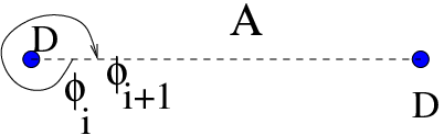
It is convenient to consider the Rényi entropies first. The Rényi entropy associated with a spatial region can be computed by taking the expectation value of a defect operator in a theory, which we denote by , obtained from taking copies of a single CFT. The operator in question is a codimension 2 defect operator localized on the boundary of a spatial region in the full Euclidean theory. In other words, the second orthogonal direction to the operator is Euclidean time. The defect operator is such that when we go around it, the various copies of the original CFT are cyclically permuted. In other words, an operator defined on the CFT is mapped to on the CFT, and is mapped to ; see Fig. 1.55 5 These defect operators are oriented: there is a which maps and a which maps . For an interval, we have the insertion of and one end and of at the other end. We will not explicitly discuss this distinction. This operator implements the boundary conditions for the replica trick [16, 17].
To analyze the light-like limit, we start from the operators in Euclidean space. We then analytically continue them to Lorentzian time. Finally, we take the light-like limit. In this limit, we expect to have an operator product expansion. This expansion differs from the standard Euclidean operator product expansion in two respects. First, we are approaching the light-like separation, where the operators have zero metric distance but do not coincide, instead of approaching the coincident point along a purely space-like displacement. Second, in dimensions, the two operators are extended and not local operators defined at a point. Despite these differences, we expect that there is a kind of operator product expansion that is applicable in this case.
To our knowledge, the systematics of operator product expansions of extended operators in the light-like limit has not been explored. For the remainder of this section, we will make reasonable physical assumptions for the form of these operator product expansions. Operator product expansions for spacelike regions were considered in [18, 19].
First, we recall the form of the light-like operator product expansion for local operators. We will take the limit with held fixed. The expansion of two scalar operators has the form
| (7) |
In this equation, the operator has spin , scaling dimension and twist ; and is the twist of the operator . The twist governs the approach to the light-like limit. For finite , we sum over all of the contributions with a given twist.
In free field theories, there are infinitely many higher spin operators with twist . These operators contain two free fields, each with twist . In an interacting theory, all operators with spin greater than 2 are expected to have twist strictly larger than . Furthermore, the twist is expected to increase as the spin increases [20] (see [21] for a more recent discussion). The only operator with spin 2 and twist is the stress tensor, unless we have two decoupled theories. Operators with spin 1 include conserved currents. Scalar operators and operators with spin can have twist , with equality only for free fields.
As noted above, for the defect operators in question are extended along some of the spatial dimensions. We now discuss features of the operator product expansion in this case. Consider first the standard Euclidean OPE (as opposed to the light-like one). For such operators, the OPE is expected to exponentiate and become an expansion of the effective action for the resulting defect operator. In general, new light degrees of freedom could emerge when the two defect operators coincide. However, in our case the two twist operators annihilate each other, leaving only terms that can be written in terms of operators of the original theory. In other words, we expect
| (8) |
where denotes the transverse dimensions and denotes local operators on the defect at . Thus the expansion is local in . We can view this equation as an expansion of the effective action for the combined defect (consisting of both defects close together) by integrating out objects with a mass scale of order .
The leading term in Eq. (8) is given by the identity operator and contributes a factor of in the exponent (with a coefficient that depends on ), where is the transverse area. This is the expected form of , which gives the vacuum Rényi entropies for the interval. In the vacuum case, all other operators have vanishing expectation values. This contribution cancels when we compute the difference of the von Neumann entropies of a general state and the vacuum, so we will not consider it further.
When we take the light-like limit of the Rényi defect operators, we expect to have an expansion which looks both like Eq. (7) and like Eq. (8). In other words, we expect the expression to be local along the direction as in Eq. (8), but with terms that are nonlocal along the direction as in Eq. (7). In principle, along the direction, we can have terms which are very nonlocal. The operator in Eq. (8) is replaced by an operator of the form on the right hand side of Eq. (7):
| (9) |
Note that the operators which appear in Eq. (9) are the operators of [18, 19]. The generic form of these operators is
| (10) |
where is an operator on the copy of the original CFT. Some of the factors in Eq. (10) could be the identity, and the simplest operators we consider have only one factor which is not the identity. Performing the replica trick, the operators with a single factor that appear in the OPE of the two defect operators contribute to the entropy proportionally to an operator in the original CFT. Specifically, we find
| (11) |
Such contributions are linear in the density matrix, and therefore do not give rise to a non-zero value of . The reason is that the operator on the right hand side is necessarily equal to , since is the only operator localized to the region whose expectation value coincides with to linear order for any deviation from the vacuum state [12] (see also [22]).
The interacting case
We will now argue that for interacting theories in , all operators that contribute to Eq. (9) are of this simple type: they all have only one nontrivial factor. In fact, only the stress tensor contributes.
Clearly, operators with will not contribute; this includes all higher spin operators in an interacting theory. Conserved spin 1 currents have twist , but cannot appear because the defect operators are uncharged. Next, consider possible contributions from operators with twist . These operators could appear in representations which are not symmetric and traceless66 6 Examples of such operators are fermion fields, or antisymmetric tensors in four dimensions. . However, since the twist operator is invariant under transverse rotations, these operators must appear in pairs; their combined twist would be bigger than .
Thus we can focus on the operators with spin zero. An operator of CFTn consisting of a single-copy scalar operator with twist in the range would contribute to the entropy. This contribution will generically be divergent in the light-like limit to , which is state dependent. In any case, single copy operators would give an equal contribution to , so these operators do not contribute to .77 7 In some cases, these contributions are not present because of symmetry reasons. An example is the Wilson-Fisher fixed point at small . In this case, the dimension of is . However, due to the symmetry, this operator does not appear in the OPE of the defect operators involved in the replica trick. Another example is the Klebanov-Witten theory [23]. These are four dimensional theories with operators of dimension . However, these operators carry a charge and cannot appear in this OPE. A relevant question here is whether there are theories with scalars with twists in this range which are not charged under any symmetry. If these operators are present, then our definition for will become divergent and will need to be modified. On the other hand, if we had two operators in the range on different CFT copies inside CFTn, the total twist will be higher than and we will not get a contribution in the light-like limit.
This leaves the stress tensor, which has and can contribute in the null limit. However, unless (in which case ), only a single factor can contribute. Therefore, for interacting theories in .
Notice that throughout this discussion, we have taken the coupling fixed and then taken the null limit. In particular, if we have a weakly coupled theory, we will get corrections to the result from free field theory which at each fixed order in perturbation theory will contain logs. One must resum the logarithms first, before taking the null limit, to recover the result that only the stress tensor survives.
Returning to the Rényi entropyies, we conclude that in interacting conformal theories, the only operator that can contribute to the expansion in the light-like limit is the stress tensor. All of its descendants contribute as well, so Eq. (9) becomes a Taylor expansion around . Discarding the contribution from the identity operator, which will drop out of , we get
| (12) |
In this expression, we have set the size of the interval and extracted an overall factor of from the exponent. This factor accounts for the vanishing of the exponent for trivial Rényi operators when . We have also replaced the sum over descendants by an integral over a function, , determined by matching with a Taylor expansion of the operator . The integral is restricted inside the null interval because operators outside this range would not commute with the operators that are spatially separated from the interval.
The difference of von Neumann entropies of a general state and the vacuum is then given by analytic continuation:
| (13) |
The function is as yet undetermined and will be further discussed in the next section.
We expect the same holds for non-conformal theories with an interacting UV fixed point. For theories with a free UV fixed point, even if we expect that the modular Hamiltonian has the same general form in terms of the stress tensor, whether or not would generically depend on further details. For relevant deformations of a free UV fixed point we expect to have as in the free theories, while we expect for asymptotically free theories.88 8 In asymptotically free theories, the coupling runs as as a function of the scale . The OPE is not given by a simple power behaviour but we need to integrate the anomalous dimensions of a range of scales as . Since , this integral diverges at short distances. Therefore, operators with non-zero anomalous dimensions do not contribute in the null limit, which involves going to very high scales. So we also expect Eq. (13) to hold.
The case of free fields or interacting fields
In free field theory, or if , states with are known to exist on a null slab [1]. We close this section by examining why the above argument for does not apply in these cases.
If the operator (10) which appears in Eq. (9) contains more than one nontrivial factor, it can give rise to a contribution to the entropy which is not equal to the expectation value of any operator in the original CFT. These contributions are interesting because they make possible. In a free field theory, such operators arise from insertions of the fundamental field in one copy and another field in another copy. They have twist and can contribute in the light-like limit.
In an interacting theory, all such operators gain a non-zero anomalous dimension. In particular, in a unitary theory, the field gains a positive anomalous dimension and so will not contribute in the null limit99 9 In gauge theories, the fundamental fields are not gauge invariant on their own, and should be supplemented with Wilson lines as interactions are turned on. These Wilson lines end at the positions of the defect.. However, in a interacting theory, multiple copies of the stress tensor can appear. Since , the total twist will remain equal to no matter how many times the stress tensor appears in (10). Thus, in , we can have even for interacting theories.
3 Properties of and Proof of the Bound
In this section, we complete the proof of the Bousso bound by establishing sufficient properties of the function in Eq. (13). We begin with a list of simple properties that are expected on physical grounds. Near each boundary of the slab, the entanglement structure is like the origin of Rindler space, and is known to hold for Rindler space from the Bisognano-Wichmann theorem [24]. Hence must satisfy
| (14) | |||||
where the last relation arises from CPT symmetry. In the remainder of this section, we will derive the remaining property crucial to the proof of the bound: .
Additional conditions arise from the theory of modular Hamiltonians. Let us define an operator on the global Hilbert space which we call the full modular Hamiltonian:
| (15) |
where is the region complementary to . For example, if is a Rindler wedge, then is proportional to the boost generator. It is known that these Hermitian operators are monotonous under inclusion [25], that is
| (16) |
is a positive definite operator for any subregion . This property can be seen as a consequence of monotonicity of relative entropy and strong subadditivity of the entropy [26]. Let us first recall the definition of relative entropy . This is positive for any two density matrices. Relative entropy can also be rewritten as
| (17) |
where and , with constant. The positivity of relative entropy implies that . Now, the monotonicity of relative entropy is the following statement. Suppose we have two regions and we have two density matricies for the big region, and . We can consider the restrictions of these density matrices to the subregion , call them and . Monotonicity is the statement that .
In the present case, we obtain two inequalities, one from and one from
| (18) | |||||
| (19) |
where we have rewritten the relative entropies using (17). Now we add these inequalities and separate the terms corresponding to the vacuum and the ones corresponding to a state different from the vacuum. The terms involving entropy are
| (20) |
which vanishes because the vacuum state is pure, and
| (21) |
which is positive due to strong subadditivity1010 10 The strong subaditivity statement we are using is where and are three disjoint systems. This property is sometimes also called weak monotonicity.. The terms with modular Hamiltonians can be grouped into and . This last term is zero since the full modular Hamiltonian is a symmetry generator which annihilates the vacuum.1111 11 This property follows from the definition and the Schmidt decomposition of the vacuum state across . Hence we end up with the inequality
| (22) |
This holds for any global state and implies (16).
Going further, Eq. (16) implies the operator inequality and hence
| (23) |
Moreover, implies , and similarly, . Subtracting both of those equations, we now have
| (24) |
In the null limit, this property is inherited by the full modular Hamiltonians of null slabs.
Now, let us consider a state whose stress-energy is positive and highly concentrated near some . Such states can be produced by taking a fixed state and boosting it. We expect that in this limit the state outside the slab (in the region , and hence also in ) is indistinguishable from the vacuum, so that , . For such states, Eq. (24) reduces to , and since both modular energies are positive,
| (25) |
Now let be a slab with and let be a slab with . The modular Hamiltonian for slabs with non-unit affine length can be obtained by a simple coordinate transformation:
| (26) |
Hence, the modular energies of the highly localized state satisfy
| (27) |
In the limit as , Eq. (25) now implies
| (28) |
Now, we repeat the argument with the region as the rindler region with , and the slab with . For this region the function . For a state with a concentrated stress tensor we obtain
| (29) |
Finally we conclude that
| (30) |
where the first inequatity is obtained from the property (14).
To prove the Bousso bound, we consider without loss of generality the null slab . We define , which obeys and by Eq. (14). We also have everywhere, by Eq. (30). These properties of the modular Hamiltonian suffice to show that the area difference along the light-sheet bounds the modular energy: (see the discussion after eqn. 4.10 in Ref. [1]). As usual, positivity of the relative entropy implies that (with equality holding for interacting theories). This completes the proof of the Bousso bound for both free and interacting theories, in the weakly gravitating limit.
4 Holographic Computation of for Light-Sheets
In this section, we consider interacting quantum field theories that have a gravity dual. In this case, the Ryu-Takayanagi formula [14, 15] allows us to compute the entropy in the null limit. This will confirm our earlier demonstration that , and will determine explicitly for such theories. First, we consider a CFT; later, we will comment on the non-conformal case. Appendix A discusses the approach to the null limit in greater detail.
We write the boundary metric as . Let us first consider a spatial strip, extended along the directions. One end of the interval is at and the other end is at , a fixed constant. The bulk metric can be written as
| (31) |
The minimal surface solution was found in [27, 28]. It is given by
| (32) | |||||
| (33) |
where is the usual hypergeometric function,1212 12 Its values at can be written in terms of gamma functions: . and is a parameter describing the first half of the minimal surface, which is symmetric around . The maximum of is achieved for . Here is the area in the directions. The formal expression for the area is UV divergent, but, as usual, we get a finite remaining contribution.
We now consider a boosted interval. For that purpose we apply a combination of a boost in the plane and a dilation that transforms
| (34) |
This transformation takes the original spacelike interval to a null interval stretched along the direction. The proper length of the interval approaches zero. We also see that the surface is approaching the AdS boundary, in the sense that the largest value of is going to zero as . Under these circumstances we find that the expression of the renormalized area (after subtracting the cutoff dependent piece) goes to minus infinity as . This is the expression for the vacuum entanglement entropy for the interval.
Let us now consider a non-vacuum state. We expect that the minimal area surface will continue to approach the AdS boundary as we take the null limit. Near the boundary, the metric approaches the AdS metric plus some small fluctuations. We can parametrize the metric as
| (35) |
Now the minimal surface action can be written as
| (36) |
where we wrote the part of the action that does not go to zero in the large boost limit, . More precisely, notice that the first two terms inside the square root scale like , while the last scales like . We will assume that and return to the case later.
The case of
For , the last term in the square root is a small perturbation and we can therefore expand the action. Due to the factor of , the resulting first order term gives a finite answer
| (37) | |||||
| (38) |
where the first term is the vacuum contribution in Eq. (33). We have also used that the vacuum contribution is larger and determines the equations of motion for the surface to the order we need in order to evaluate the second term. We then see that the component of the metric gives a finite contribution. By performing a similar expansion, we can check that all other components of the metric do not contribute in the null limit either. For this, it is important to use (34) to see how various terms behave. As an example, consider a component in the metric. The component contains a which multiplies the whole action that scales as . Since , such a term does not contribute. In a similar way, we discard higher orders in in the expansion of the metric around .
In conclusion, the only part of the metric that matters is the first non-zero term in the expansion of . This first-order term is also the term that gives the expectation value of the stress tensor,
| (39) |
where is the value of the stress tensor (we have set the AdS radius to unity). A similar expansion was performed in [12].1313 13 The authors of [12] considered a general surface and then expanded the metric to first order around the AdS metric. Here, the argument is simpler because we only need the first order term in the expansion of the metric near the boundary. Furthermore, we only need to consider the component. Using the solution (32), we can write (38) in the form
| (40) |
with defined parametrically by
| (41) |
The function is plotted for several dimensions in figure 2. Explicitly, we find for , and in the limit the function converges to . For small , we obtain the result .
We have thus obtained in terms of the expectation value of an operator, namely a certain integral of . According to the general argument discussed in Sec. 2, the operator in the right hand side is ; we obtain .

Notice that the relation gives values of the entropy on the light-sheet that are very different from naive expectations. For example, consider a thermal state. The entropy scales with the size of the interval as , rather than the naïve (volume-extensive) entropy which grows like and which applies in the large temperature regime. Hence in this regime, we find is actually much greater than the naive entropy. To check in detail how the extensive entropy for spatial regions turns into a term that goes as for null surfaces, we have computed the areas of minimal surfaces in a black hole background. We find that there is actually a phase transition into a different class of extremal surface solutions as . This is explained in more detail in Appendix A.
We can now briefly discuss the situation in non-conformal field theories. If we add a relevant deformation to the field theory, we are adding a scalar field in the bulk which has a profile going like for small . This affects the metric at quadratic order via terms of the form . Such terms modify only the diagonal components of the metric, and we have seen that as long as , such terms vanish. The latter is precisely the unitarity condition for a non-free scalar operators. 1414 14 The unitarity condition is . For equality, we have a free field in the boundary theory.
The case of
In two dimensions, it is still true that the minimal surfaces (geodesics) approach the boundary, but it is no longer true that we can treat the term involving in a perturbative fashion because it scales in the same way as the other terms. This implies that the final answer is non-linear in . This non-linearity allows for .
For simplicity, consider the special case of the theory at finite temperature (or in Rindler space). Since it is related by a conformal transformation to the plane, we can do all the computations explicitly by a simple coordinate transformation. The two point function of the twist operators is
| (42) |
with . This leads to the entropy [17]
| (43) |
The vacuum case is given by the limit, or . In the null limit we get
| (44) |
This can be expanded as
| (45) | ||||||
| (46) |
where . The first line is what we expect from the expansion of terms involving operators of the form , possibly integrated at different points, replica copies, etc. The last expression comes from resuming all these operators. In this case, this agrees with what we expect from the operator product expansion, since all these operators have twist zero in . The important point is that operators on different replica copies survive the limit; see Sec. 2.
5 Why is on Null Surfaces?
The relation is startling at first sight. It implies that the relative entropy between any state and the vacuum, , vanishes in the light-like limit. The relative entropy is a statistical measure of how easy is to differentiate between two states by making measurements. In general, the probability of confounding two states by making measurements falls off exponentially no faster than (see e.g. [29]). If , then the vacuum cannot be differentiated from any other state by making measurements of operators localized to a null surface. In other words, all states look the same as we approach this surface.
A related puzzle is the following: it is a general property of relative entropy that implies , but this in turn would give . However, the prediction is not what we have found holographically.

In this section, we explain both of these puzzles by noting that the quantities and are defined as limits for vanishing . At finite , the states are distinguishable by operators included in the algebra on the causal development of the spatial interval, but as we take the limit , any fixed operator eventually drops out from the algebra. No operator remains in the intersection of all algebras, =1.1515 15 Note that the operator evaluated on the null interval should not be considered as part of the algebra because it sends states into non-normalizable states, even if we smear the operator along the null interval and the transverse directions. Nevertheless, the expectation value of this operator can be computed and can be different in two different states. See figure 3. The same reason explains how and can be non-zero while the relative entropy is zero. This result cannot be correct for states on a fixed algebra, but it is a possibility for these quantities defined as limits on vanishing algebras. We describe how this can be accomplished using a toy model of an infinite chain of qubits in appendix B.
In general, the relation could not have been possible if the algebras for finite were not infinite dimensional. This phenomenon requires the full QFT, taking the UV cutoff to zero before taking . Otherwise, at finite , we would run out of operators and find .
Let us briefly describe what is meant by a full quantum field theory. A quantum field is an operator-valued distribution. In order to produce an operator acting on Hilbert space, a quantum field has to be averaged by a smooth function of compact support . If is smooth on a -dimensional spacetime region, we are guaranteed by the Wightman axioms that is a well defined operator whose domain contains the vacuum state. The set of these operators where the support of is included in a spacetime region generates the algebra of operators acting in .1616 16 These are von Neumann algebras. There is a technical point in that these algebras are better described as algebras of bounded operators. Bounded operators can be obtained from by taking the projectors in its spectral decomposition [30].
We want to see if a fixed localized operator can be defined for the null plane such that it remains in the intersection of the algebras which implement the null limit. The problem of whether the domain of the test function can be reduced to a spatial region or a region on a null plane, as opposed to a spacetime region, was studied in the past [31, 32], mainly in attempts to develop a precise mathematical foundation to the usual canonical formalism of equal time commutation relations (see also [10]). If is a well-defined operator, we should have
| (48) |
This condition on the two point function of the field constrains its ultraviolet behavior.
The Fourier transform of the two point function with no time ordering is
| (49) |
where is a polynomial in the transverse components. To evaluate Eq. (48), we take the Fourier transform:
| (50) |
For with support on the surface , we have
| (51) |
with independent of and falling off to zero faster than any polynomial in and due to the smoothness of . We have
| (52) |
The test function makes the integral convergent for large and . However, the integral may not converge for large . The best chance we have for it to converge is when . Power counting gives a convergent integral if
| (53) |
which is never the case for a unitary theory.
For free fields, we have , but the field obeys the wave equation so that instead of Eq. (49), we have an expression localized on the mass shell . In this case, the denominator in Eq. (49) is replaced by the delta function . Eliminating gives
| (54) |
This integral in is logarithmically divergent for a free scalar field with , but converges for and its derivatives with . For a free spin field, it converges for the component (and derivatives). For a Maxwell field tensor , we must again take the component with and , that is, the components .
So only for free fields do we expect to have operators localized on the null surface and for general states. The localized operators can be non-local in the direction so that does not need to decompose into a sum of contributions from each of the null lines.
For non-conformal theories with a free UV fixed point, the localizability of the operators depends on the details of the approach to the fixed point. Using the spectral representation of the two point function for a scalar field in terms of that of a free massive scalar field
| (55) |
the general result [32] is that the derivative of this scalar field can be localized only if
| (56) |
This condition gives a finite wave function renormalization, which is expected to hold for superrenormalizable theories but not for marginal renormalizable theories [33].
6 Conclusions
Summary.
We explored some properties of the entropy associated to null slabs in general interacting field theories. We found a general expression for the modular Hamiltonian in terms of a local integral of the stress tensor components along the null slab, Eq. (2). We derived this by considering the light-cone OPE for the defect operators that compute the Rényi entropies; general arguments involving the spectrum of operators then constrain the von Neumann entropy and show that it is equal to the modular Hamiltonian.
We also proved certain inequalities obeyed by the function that multiplies the stress tensor in the modular Hamiltonian. These inequalities, Eqs. (28) and (30), were previously shown [1] to be sufficient for the Bousso bound [2]. Our work extends our earlier proof of the Bousso bound to interacting theories.
We computed the entanglement entropy in the null limit for theories with a gravity dual. In the null limit, the minimal surface approaches the AdS boundary. The change in the area can be found from the asymptotic form of the metric. This asymptotic form of the metric also determines the stress tensor. Therefore, we get a result that is in line with our general expectations. We view this as an additional consistency test on the holographic entanglement entropy formula [14, 15] in a strongly Lorentzian context. Our analysis fully determines the function for such theories, Eq. (41), and it shows that takes a different form than in the free theory.
A curious feature of our result is that, for interacting theories, the change in entropy is exactly given by the change in the expectation value of the modular Hamiltonian: . In a finite-dimensional Hilbert space, this relation would also imply that both and are zero. Here, however, they are non-zero. This is possible because we are taking a limit that involves infinite dimensional algebras. We also saw that no elements remain in the algebra after we take the limit. One can still consider limiting values of expectation values of operators on the null line, but such operators, or their smeared versions on the null surface, do not define reasonable operators on the Hilbert space because their variance is infinite. Physically, this result means that in interacting theories, one cannot distinguish between any two states by making measurements purely on the light-sheet. Appendix B presents a simple toy model involving an infinite number of qubits where similar features are present.
Discussion and open problems.
The Bousso bound involves the notion of an entropy flux through the light-sheet. Defining a local notion of entropy current is notoriously difficult in quantum field theory. Here we have defined it through , the difference in the von Neumann entropies of the interval between two different quantum states. This notion does indeed have properties that suffice to ensure the validity of the corresponding Bousso bound. Nevertheless, the quantity has some counter-intuitive properties.
The most surprising aspect of this definition is that we find , which means that all ordinary states are indistinguishable by local measurements on the light-sheet. We have not found more familiar-looking definitions for the entropy flux, to which a Bousso-type bound might apply. Further research will be needed to better understand the relation between and more conventional (spacelike) definitions for the entropy flux.
Notice that the energy flux is given by a local quantity, the expectation value of . On the other hand, is non-local since the function depends on the positions of the endpoints of the interval. Thus, it cannot be viewed as the flux of a local operator.
We expect that will provide an upper bound to the more familiar concepts of entropy. For example, in a theory where we can define an entropy current, as in hydrodynamics, we expect that should be larger than the flux of the entropy current on the light-sheet. In the holographic computations involving black branes, this is indeed true. The reason is very simple: the entropy flux scales like the length of the interval, , on the other hand scales like . The relative coefficient involves the temperature, . This means that if is somewhat greater than , then will be larger than the entropy flux. We also see this clearly in the two dimensional results, Eq. (44). We expect this to be a general feature of thermal or hydrodynamic states.
An interesting conclusion is that information in interacting theories becomes very delocalized on the light front. Information that is fairly localized along the longitudinal direction in free theories spreads once we include interactions. We also expect that the mutual information between a null interval and any other fixed region should vanish. This follows from the result . We also see this in the holographic examples.
In a CFT with a gravity dual, the entropy for spatial slabs in a thermal state displays a phase transition as the null limit is approached (see Appendix A). This is likely to hold in general for states which start out with a non-zero for a spacelike interval in the large approximation.
For free theories, one can prove not only the covariant bound but the stronger result of monotonicity [1]: never decreases under inclusion in a larger light-sheet. This follows from the concavity of the function , , which holds in the free case. Here, we found that this property continues to hold for interacting theories with a holographic dual (Fig. 2), so monotonicity of follows in these cases. We leave a general proof of to future work. It would also be nice to compute the function to first order in perturbation theory for a weakly coupled CFT, such as super Yang-Mills.
Acknowledgements.
We thank D. Marolf and A. Wall for discussions. R.B. and Z.F. are supported in part by the Berkeley Center for Theoretical Physics, by the National Science Foundation (award numbers 1214644 and 1316783), by the Foundational Questions Institute grant FQXi-RFP3-1323, by “New Frontiers in Astronomy and Cosmology”, and by the U.S. Department of Energy under Contract DE-AC02-05CH11231. H.C. thanks the Institute for Advanced Study for hospitality and financial support. H.C. is partially supported by CONICET, CNEA, and Univ. Nac. Cuyo, Argentina. J.M. is supported in part by U.S. Department of Energy grant DE-SC0009988.Appendix A Extremal Surfaces and Phase Transitions on a Black Brane Background
In this appendix, we consider a thermal state in an interacting CFT with a bulk dual, an asymptotically anti-de Sitter planar black brane spacetime. This allows us calculate the entanglement entropy holographically using the HRT prescription [15]. We are able to study the approach to the null limit in detail, showing that the entropy on sufficiently large slabs undergoes a phase transition at large boost. We reproduce the result for the null slab.
The metric of a black brane in AdS is
| (57) |
The inverse black hole temperature is
| (58) |
and the energy density is given by
| (59) |
It follows that the null-null component of the stress tensor is
| (60) |
The extremal surface action is
| (61) |
Let the momentum conjugate to be denoted . We find
| (62) |
Define a new effective Lagrangian :
| (63) |
Writing for the momentum conjugate to , we obtain
| (64) | |||||
| (65) | |||||
| (66) |
These are the equations of motion of the extremal surfaces. We take and fix scale invariance by setting in the function , so . Integrating these trajectories, we obtain the null coordinates of the the extremal surface solutions at the boundary,
| (67) |
We can also rewrite the initial action (i.e. area) from Eq. (61) as
| (68) |
In these integrals, the upper limit is the return point of the trajectory, which is the smallest positive root of the denominators of Eqs. (65) and (66); that is,
| (69) |
The turning point is calculated from the smallest solution of this equation, with . The first two terms in Eq. (69) are positive when , and the second is greater than one. We conclude that an extremal surface which returns to the boundary exists for all . As we increase from zero with , there are solutions for only up to a maximum value of , which we denote by . This maximum value of is simultaneously the solution to Eq. (69) and
| (70) |
When , there are no extremal surface solutions that return to the AdS boundary.

In Fig. 4, we plot the parameter space for . In , the curve runs near the line ; the plot looks similar in other dimensions. The shaded region contains the extremal surface solutions.
Interestingly, the extremal surface for corresponds to a time-like region on the boundary, with . This counter-intuitive result is possible because even if the boundary interval is time-like, we are still considering locally spatial surfaces in the bulk. However, these extremal surfaces cannot be regulated by vacuum-subtraction, because the extremal surface solutions with this boundary region in vacuum AdS do not have a well-defined area. So the parameter space we are interested in is further reduced to , where denotes the energy for which the extremal surface solution has .
The separation between and in parameter space is, however, exponentially small. We show the relevant contour in figure in Fig. 5 in logarithmic variables (for ; other dimensions are similar).
Numerical analysis of the solutions shows that, for and smaller1717 17 Recall we have set to unity., there are no exact solutions with , only an asymptotic set of solutions for which is fixed and approaches but never exactly reaches zero. The parameters and go to infinity in the limit , and the extremal surface runs closer to the AdS boundary. We call this family of solution the “perturbative solutions,” because can be computed perturbatively in this case (see Sec. 4). For sufficiently large (larger than approximately in ), in addition to the asymptotic solution, there exist two other solutions with finite such that exactly. Fig. 5 gives the contour plot of and for a region of the parameter space . We plot the solutions in logarithmic parameter space in Fig. 5. Following a contour of constant and sufficiently large from left to right in this diagram, , we intersect the contour twice, corresponding to the two precisely null solutions. The part of the contour to the left of the first intersection (with ) is the “thermal” family of solutions. These solutions have a thermal character because most of the surface extends near to the horizon of the black hole. Hence the entropy contains a term that grows like , a volume-extensive term that goes with the thermal entropy density. By increasing along a contour of fixed , we again approach the asymptotic perturbative solution.

Let us see in more detail how the area behaves in these two solutions. As shown below, there is a third null solution, but it has greater area than the other two and, according to the HRT prescription, should not be regarded as the entropy.
Perturbative solution
According to Sec. 4, we expect the limiting value of the entropy to take the form
| (71) |
The difference between the perturbative extremal surface area and the vacuum area is
| (72) |
Using Eq. (60) and the explicit form of the function , we obtain
| (73) |
Setting , we obtain perfect accord with our numerical simulation of the extremal surfaces.
Thermal solution
This solution captures the thermal entropy. We expect the difference in extremal surface areas to approach asymptotically at large .
The thermal solutions track the horizon of the black hole at . In parameter space, this occurs when is of the same order as . When this is the case, most of the contribution to the integral comes from the region where is order , and we can expand the integrand around that point.
First we perform the substitutions
| (74) |
In this limit, the integrals become
| (75) | |||||
| (76) | |||||
| (77) |
The renormalized area is obtained by subtracting the divergent piece with a UV cutoff . Note that the zeros in the denominator occur at , both of which we take to be positive. Additionally, there is a zero at in the denominator of the integral for . The integral over starts at the largest zero, , and moves to larger values of (which corresponds to smaller values of ). We can do these integrals and focus on the potentially large terms at small . We obtain
| (78) | |||||
| (79) | |||||
| (80) |
The last equation implies that the entropy flux is what we expected. We take the ansatz with , where is some constant. The expansions become, for small ,
| (81) | |||||
| (82) |
Setting for the null solution, we find
| (83) |
This means that thermal solutions with exact exist for large .
However, we are interested not in the renormalized area but in the area difference with respect to the vacuum solution. Using the area for the vacuum solution [28], the area difference for large is
| (84) |
Phase transition for large
Comparing Eqs. (73) and (84), wee see that the perturbative solution has less area than the thermal one for sufficiently small . This occurs because the perturbative solution has the same negative and finite term as the vacuum solution which grows like . Hence this term does not appear in the area difference in Eq. (73). The thermal solution cannot have this term because it is an exact solution valid for ; its area cannot depend on . Therefore, the area difference, Eq. (84), diverges as for the thermal class of solutions. However, for finite values of and sufficiently large values of , the thermal solution must have smaller area, since it increases only linearly with while the perturbative solutions grow quadratically. The phase transition occurs when the area of the two solutions becomes equal, which is approximately given by
| (85) |

We have numerically evaluated as a function of for fixed in dimensions. The result is shown in Fig. 6. We observe that, as predicted, the thermal solution tends toward infinite area as we take the limit . One of the perturbative solutions becomes the minimal area solution for at some finite . In every case, the minimal area plateaus to a finite, non-zero value as .
Appendix B Toy Model with
In this appendix, we present a toy model with a countable number of degrees of freedom (qubits), which shares the property we found for interacting theories on a null slab: . This relation is only possible as a limiting statement, because zero relative entropy between two states and implies that the states are equal. Moreover, the relation requires an infinite number of degrees of freedom, or else it would be reached before the limit is taken, in contradiction with the previous sentence.
To demonstrate the effect in a toy model, we construct a decreasing sequence of algebras from which any fixed bounded operator will disappear as ; in other words, only contains multiples of the identity operator. Consider an infinite sequence of qubits. The algebra generated by the qubits operators for the qubits at position will be denoted by . The algebras are nested: for . The relative entropy of two states reduced to will decrease with ; that is, .
Consider states which are formed by tensor products of two-qubit states for the and qubits. This choice for the entanglement is arbitrary, but entanglement between the qubits and with growing much faster than is necessary to generate more entanglement than the entropy that is lost as we trace over the first qubits.
Entanglement plays an important role in keeping finite while the relative entropy goes to zero. The classical entropy is monotonous, so without quantum entanglement, the entropies must tend to zero with increasing . In the quantum case, the entropy is no longer monotonous, but the relative entropy is monotonous and tends to zero instead.
Consider generic states of the form
| (86) |
In this tensor product, we omit if is already included in the product by a previous factor of with . The global relative entropy of two states both of the form in Eq. (86) is
| (87) |
We want a finite relative entropy, so a convergent series. We construct a sequence of mixed states by tracing over the first qubits of . As tends to infinity, the relative entropy approaches zero:
| (88) |
where we have used that the positivity of the relative entropy, and the fact that the relative entropy of two states on a pair of qubits is greater than that of the states reduced to the second qubit of the pair.
We want the global to remain finite as goes to infinity:
| (89) |
For the sequence of entropies , we have
| (90) |
Here, denotes the entropy of the reduced states on the second qubit of the pairs. The pairs of qubits with have been completely traced out, while the pairs with are still completely included in the state.
Using Eq. (89), we see that the first sum in Eq. (90) tends to zero as . For the second sum to have a finite and positive limit, we demand
| (91) |
which gives
| (92) |
If decays much faster, we get , which is not what we want. To get a non-zero answer, the entropy of the pairs must not be integrable. If it decays at a slower asymptotic rate than Eq. (91), the limiting value of is infinity.
Now we choose the two qubit states and . We impose three conditions: the relative entropies of these pairs should be integrable, Eq. (88); the differential entropies of these pairs should also be integrable, Eq. (89); and the of the states on the second qubit should have the asymptotic form in Eq. (91), or slower than this if we want to obtain .
We choose the pair of states to be
| (93) | |||
| (94) |
with , a pair of orthogonal pure states for the two qubits. (We choose mixed states because the relative entropy diverges for any two non-identical pure states.) Taking to be small, we find
| (95) | |||
| (96) |
Here, and depend on the pair of qubits , and the dependence on is such that these entropies are integrable.
To evaluate the reduced entropy, we have to specify the pure states in terms of the qubits. The choice is arbitrary, but there are some restrictions. We cannot choose two orthogonal maximally entangled states for and , because in this case, the reduced density matrices and will both equal and we obtain . Instead, we take the two orthogonal states
| (97) | |||||
| (98) |
Then the entropy is
| (99) |
We can tune the dependence of on so that the entropy goes as Eq. (91) and both Eq. (95) and Eq. (96) are integrable. We fix and and take . The relative entropy is integrable because it contains a higher power of . For the total to be finite, we can choose , to get an additional power of from the logarithm term in Eq. (96). Then the states converge to a random state in the sub-Hilbert space spanned by . With this choice, both the total and the relative entropy are finite; the relative entropy goes to zero with , while the limit of is
| (100) |
It is also clear that we have in the limit, or equivalently the relative entropy goes to zero.
The limit for can be made much larger (or infinite) by slowing the asymptotic decay of . For example, keeping , and as before but setting causes to diverge with finite initial , while the relative entropy remains constant.
References
- (1) R. Bousso, H. Casini, Z. Fisher, and J. Maldacena, “Proof of a Quantum Bousso Bound,” arXiv:1404.5635 [hep-th].
- (2) R. Bousso, “A covariant entropy conjecture,” JHEP 07 (1999) 004, hep-th/9905177.
- (3) E. E. Flanagan, D. Marolf, and R. M. Wald, “Proof of Classical Versions of the Bousso Entropy Bound and of the Generalized Second Law,” Phys. Rev. D 62 (2000) 084035, hep-th/9908070.
- (4) G. ’t Hooft, “Dimensional reduction in quantum gravity,” gr-qc/9310026.
- (5) L. Susskind, “The World as a hologram,” J. Math. Phys. 36 (1995) 6377–6396, hep-th/9409089.
- (6) W. Fischler and L. Susskind, “Holography and cosmology,” hep-th/9806039.
- (7) R. Bousso, “The holographic principle,” Rev. Mod. Phys. 74 (2002) 825, hep-th/0203101.
- (8) H. Casini, “Relative entropy and the Bekenstein bound,” Class.Quant.Grav. 25 (2008) 205021, arXiv:0804.2182 [hep-th].
- (9) D. Marolf, D. Minic, and S. F. Ross, “Notes on space-time thermodynamics and the observer dependence of entropy,” Phys.Rev. D69 (2004) 064006, arXiv:hep-th/0310022 [hep-th].
- (10) A. C. Wall, “A proof of the generalized second law for rapidly changing fields and arbitrary horizon slices,” Phys.Rev. D85 (2012) no. 6, 104049, arXiv:1105.3445 [gr-qc].
- (11) G. Lindblad, “Entropy, Information and Quantum Measurements,” Commun. Math. Phys. 33 (1973) 305.
- (12) D. D. Blanco, H. Casini, L.-Y. Hung, and R. C. Myers, “Relative Entropy and Holography,” JHEP 1308 (2013) 060, arXiv:1305.3182 [hep-th].
- (13) J. Maldacena, “The Large limit of superconformal field theories and supergravity,” Adv. Theor. Math. Phys. 2 (1998) 231, hep-th/9711200.
- (14) S. Ryu and T. Takayanagi, “Holographic derivation of entanglement entropy from AdS/CFT,” Phys.Rev.Lett. 96 (2006) 181602, arXiv:hep-th/0603001 [hep-th].
- (15) V. E. Hubeny, M. Rangamani, and T. Takayanagi, “A Covariant holographic entanglement entropy proposal,” JHEP 0707 (2007) 062, arXiv:0705.0016 [hep-th].
- (16) J. Callan, Curtis G. and F. Wilczek, “On geometric entropy,” Phys.Lett. B333 (1994) 55–61, arXiv:hep-th/9401072 [hep-th].
- (17) P. Calabrese and J. Cardy, “Entanglement entropy and conformal field theory,” J.Phys. A42 (2009) 504005, arXiv:0905.4013 [cond-mat.stat-mech].
- (18) M. Headrick, “Entanglement Renyi entropies in holographic theories,” Phys.Rev. D82 (2010) 126010, arXiv:1006.0047 [hep-th].
- (19) J. Cardy, “Some results on the mutual information of disjoint regions in higher dimensions,” J.Phys. A46 (2013) 285402, arXiv:1304.7985 [hep-th].
- (20) O. Nachtmann, “Positivity constraints for anomalous dimensions,” Nucl.Phys. B63 (1973) 237–247.
- (21) Z. Komargodski and A. Zhiboedov, “Convexity and Liberation at Large Spin,” JHEP 1311 (2013) 140, arXiv:1212.4103 [hep-th].
- (22) G. Wong, I. Klich, L. A. Pando Zayas, and D. Vaman, “Entanglement Temperature and Entanglement Entropy of Excited States,” JHEP 1312 (2013) 020, arXiv:1305.3291 [hep-th].
- (23) I. R. Klebanov and E. Witten, “Superconformal field theory on three-branes at a Calabi-Yau singularity,” Nucl.Phys. B536 (1998) 199–218, arXiv:hep-th/9807080 [hep-th].
- (24) J. Bisognano and E. Wichmann, “On the Duality Condition for Quantum Fields,” J.Math.Phys. 17 (1976) 303–321.
- (25) H. Borchers, “On the use of modular groups in quantum field theory,” Annales Poincare Phys.Theor. 63 (1995) 331–382.
- (26) D. D. Blanco and H. Casini, “Localization of Negative Energy and the Bekenstein Bound,” Phys.Rev.Lett. 111 (2013) 221601, arXiv:1309.1121 [hep-th].
- (27) D. E. Berenstein, R. Corrado, W. Fischler, and J. M. Maldacena, “The Operator product expansion for Wilson loops and surfaces in the large N limit,” Phys.Rev. D59 (1999) 105023, arXiv:hep-th/9809188 [hep-th].
- (28) S. Ryu and T. Takayanagi, “Aspects of Holographic Entanglement Entropy,” JHEP 0608 (2006) 045, arXiv:hep-th/0605073 [hep-th].
- (29) V. Vedral, “The role of relative entropy in quantum information theory,” Rev.Mod.Phys. 74 (2002) 197–234.
- (30) R. Haag, Local Quantum Physics: Fields, Particles, Algebras. Springer Verlag, Berlin, 1992.
- (31) O. Steinmann, “Structure of the Two-Point Function,” Journal of Mathematical Physics 4 (1963) no. 5, 583–588.
- (32) S. Schlieder and E. Seiler, “Remarks on the null plane development of a relativistic quantum field theory,” Commun.Math.Phys. 25 (1972) 62–72.
- (33) R. Streater, “Outline of Axiomatic Relativistic Quantum Field Theory,” Rept.Prog.Phys. 38 (1975) 771–846.