Quenching and anisotropy of hydromagnetic turbulent transport
Abstract
Hydromagnetic turbulence affects the evolution of large-scale magnetic fields through mean-field effects like turbulent diffusion and the effect. For stronger fields, these effects are usually suppressed or quenched, and additional anisotropies are introduced. Using different variants of the test-field method, we determine the quenching of the turbulent transport coefficients for the forced Roberts flow, isotropically forced non-helical turbulence, and rotating thermal convection. We see significant quenching only when the mean magnetic field is larger than the equipartition value of the turbulence. Expressing the magnetic field in terms of the equipartition value of the quenched flows, we obtain for the quenching exponents of the turbulent magnetic diffusivity about 1.3, 1.1, and 1.3 for Roberts flow, forced turbulence, and convection, respectively. However, when the magnetic field is expressed in terms of the equipartition value of the unquenched flows these quenching exponents become about 4, 1.5, and 2.3, respectively. For the effect, the exponent is about 1.3 for the Roberts flow and 2 for convection in the first case, but 4 and 3, respectively, in the second. In convection, the quenching of turbulent pumping follows the same power law as turbulent diffusion, while for the coefficient describing the effect nearly the same quenching exponent is obtained as for . For forced turbulence, turbulent diffusion proportional to the second derivative along the mean magnetic field is quenched much less, especially for larger values of the magnetic Reynolds number. However, we find that in corresponding axisymmetric mean-field dynamos with dominant toroidal field the quenched diffusion coefficients are the same for the poloidal and toroidal field constituents.
Subject headings
Magnetohydrodynamics – convection – turbulence – Sun: dynamo, rotation, activityI. Introduction
Many astrophysical objects possess turbulent convection, and the dynamo mechanisms based on it are believed to be responsible for the generation and maintenance of the observed magnetic fields. The study of the dynamo mechanism in the solar convection zone using simulations of turbulent convection in spherical shells began in the 1980s with the works of [27], [26] and [28], and has recently been pursued further by many more authors [13, 67, 43, 44, 50]. However, under stellar conditions the dimensionless parameters governing magnetohydrodynamics attain extreme values, which are far from being accessible through numerical models. So we do not know to what extent feasible models at temperate parameter regimes reflect properties of convection and dynamos in real stars. An alternative approach to studying the dynamo problem is mean-field theory which began with the pioneering works of [62], [2], and [89]. This approach is computationally less expensive because one needs not to resolve the full dynamical range of the small-scale turbulence, which is instead parameterized. In recent years, there have been significant achievements of mean-field MHD in reproducing various aspects of magnetic and flow fields in the Sun [19, 71, 39, 20, 21, 45, 17, 64, e.g.,].
In this context, an important task is to determine the mean electromotive force , which results from the correlation between the fluctuating constituents of velocity and magnetic field, in terms of the mean field . There is no accurate theory to accomplish this task from first principles, except for some limiting cases, in particular those of small Strouhal and magnetic Reynolds number, . Therefore, suitable assumptions are required in determining . When varies slowly in space and time, we may write
| (1) |
The diagonal components of are usually the most important terms for dynamo action, but in the presence of shear, the [56] and shear-current [79] effects, both covered by , can also enable it. Many components of , however, describe dissipative effects.
Doubts can be raised regarding the explanatory and predictive power of mean-field dynamo models given that the tensors and are often chosen to some extent arbitrarily or even tuned to obtain results resembling features of the Sun. Therefore, methods to measure these coefficients from simulations have been developed. At present the most accurate method is the so-called test-field method [87, 88, 8, 10]. In this method, one selects an adequate number of independent mean fields, the ‘test fields’, and solves for each of them the corresponding equation for the fluctuating magnetic field (in addition to the main simulation). Finally, via computing the mean electromotive force, the transport coefficients are calculated.
There are different variants of the test-field method. The best established one is based on the average over two spatial (the ‘horizontal’) coordinates. This method has been applied to a large variety of setups, e.g., isotropic homogeneous turbulence [92, 8], homogeneous shear flow turbulence [9], with and without helicity [58], turbulent convection [41], and supernova driven interstellar turbulence [29]. Another variant is based on Fourier-weighted horizontal averages and allows to determine also the coefficients that multiply horizontal derivatives of the mean field. This method has been applied to forced turbulence [7] and to cosmic ray-driven turbulence [81, 14].
In models based on thin flux tubes, forming the major alternative to distributed turbulent dynamos, the magnetic field strength in the deep parts of the solar convection zone is believed to exceed its value at equipartition with velocity [18, 23, 95]. On the other hand, it is well known that turbulent transport becomes less efficient when the mean magnetic field’s strength is comparable to or larger than the equipartition value. Therefore precise knowledge of the quenching is needed. Mean-field dynamo models of the type often employ an ‘ad hoc’ algebraic or dynamical -quenching [36, 22], while largely ignoring the quenching of the turbulent diffusivity despite of its importance in determining the cycle frequency. Indeed, in the absence of quenching, the standard estimate of for the Sun (–) yields a rather short cycle period of – [55]. However, by considering the quenching of , a reasonable value of the cycle period can easily be obtained [86, 31, 60]. In fact, measuring the cycle frequency in a simulation has been one way of determining the quenching of [38].
Early work by [59] and [82] showed that under the Second Order Correlation Approximation (SOCA), is quenched inversely proportional to the third power of the magnetic field. Following [93], several investigations have suggested that is beginning to be quenched noticeably when the mean field becomes comparable to times the equipartition value [16], i.e., for extremely weak magnetic fields. This behavior is also called ‘catastrophic quenching’. However, it is now understood as an artifact of having defined volume-averaged mean fields [3, 8] combined with the usage of perfectly conducting or periodic boundary conditions and is not expected to be important in astrophysical bodies where magnetic helicity fluxes can alleviate catastrophic quenching [54, 24, e.g.,]. The actual value of shows a much weaker dependence on even when is comparable with the equipartition value [8]. This work also shows that the dependence of and is such that their contributions to the growth rate nearly balance, with a residual matching the microscopic resistive term. This is in fact a requirement for the dynamo to be in a saturated state. Consequently the saturated mean electromotive force is proportional to , which is sometimes misinterpreted as catastrophic quenching.
Once catastrophic quenching is alleviated, the magnetic field can grow to equipartition field strengths, when other quenching mechanisms that are not dependent might become important and can therefore be studied already for smaller values of . [91] found that is quenched proportional to and for time-dependent and steady flows, respectively. Their latter result was based on analytic theory and appeared to be confirmed by numerical simulations using a steady forcing proportional to the ABC-flow. However, subsequent work by [72] demonstrated quenching proportional to for a steady forcing proportional to the flow I of [75], hereafter referred to as Roberts flow. They also noted that for ABC-flow forcing the quenching is indeed better described when setting the power also to 4 instead of 3. More recently, in supernova driven turbulent dynamo simulations, Gressel et al. [29] find where is the local equipartition value.
For the turbulent diffusivity, [52] and [77] obtained that is quenched inversely proportional to . In the two-dimensional case, [15] have found catastrophic quenching of . However, this is a special situation connected with the fact that in two dimensions the mean square vector potential is a conserved quantity. This is no longer the case in three dimensions. Quenching similar to [52] has been confirmed by simulations [3, 1, 29]. In particular, making the ansatz , [29] find in supernova-driven simulations of the turbulent interstellar medium. On the other hand, [97] find in simulations of forced turbulence with a decaying large-scale magnetic field. However [38] found that their results depend on the strength of shear and found for weak shear while for strong shear.
In the present work we measure the quenching of these transport coefficients as a function of the mean magnetic field strength for three different background simulations – (i) a forced Roberts flow, (ii) forced turbulence in a triply periodic box, and (iii) convection in a bounded box. In all these simulations we impose a uniform and constant external mean field. However, this induces a preferred direction which causes the statistical properties of the turbulence to be axisymmetric with respect to the direction of the magnetic field. In the following, we refer to such flows as axisymmetric turbulence, for which the number of independent components of the and tensors is reduced to only nine, simplifying also their determination [7].
II. Concept of turbulent transport in mean-field dynamo
The evolution of the magnetic field in an electrically conducting fluid is governed by the induction equation
| (2) |
where is the fluid velocity. Here, is the microphysical magnetic diffusivity, while the magnetic permeability of the fluid has been set to unity. Thus the current density is given by . In mean-field MHD, we consider the fields as sums of ‘averaged’ and small-scale ‘fluctuating’ fields, with the assumption that the averaging satisfies (at least approximately) the Reynolds rules. Denoting averaged fields by overbars and fluctuating ones by lowercase letters, we write the equation for the mean magnetic field as
| (3) |
where is the aforementioned mean electromotive force, which captures the correlation of the fluctuating fields and . The ultimate goal of mean-field MHD is to express in terms of itself. There are several procedures for doing that. When the mean magnetic field varies slowly in space and time we can write in the form of Equation (1). Our primary goal is to measure the transport coefficients and in the presence of an imposed uniform magnetic field and, in particular, measure the degree of their quenching and anisotropy.
Let us consider turbulence that is anisotropic and exhibiting only one preferred direction , referring to an external magnetic field, rotation axis, or the direction of gravity. Then following [7], the general representation of is given by
| (4) | ||||||||||||
with nine coefficients , , , . While is given by the antisymmetric part of the gradient tensor , is defined by with being the symmetric part of . For homogeneous isotropic turbulence , and the other coefficients vanish. We note that our sign convention for , , and follows that commonly used, but it differs from that used in [7].
The term corresponds to a modification of turbulent diffusion along the preferred direction. To understand this, let us assume that only , , and are non-vanishing and independent of position. By introducing the quantities with and , we have
| (5) |
which shows that positive values of correspond to an enhancement of turbulent diffusion along the preferred direction. As Equation (5) reveals, and do not characterize the diffusion parallel and perpendicular to the preferred direction, as their symbols might suggest.
An anisotropy similar to that of Equation (5) has been considered in connection with the turbulent decay of sunspot magnetic fields [85], where the mean magnetic field defines the preferred direction. It has not yet been used in mean-field dynamo models, where, however, anisotropies of the turbulent diffusivity due to the simultaneous influence of rotation and stratification have been taken into account [83, 65] .
III. The Model Setup
We distinguish two basically different schemes of establishing the background flow: by a prescribed forcing or by the convective instability. In the first case, both laminar and turbulent (artificially forced) flows will be considered. With respect to the fluid, we generally think of an ideal gas with state variables density , pressure and temperature , adopting, however, different effective equations of state for the two schemes.
The continuity and induction equations are shared by both schemes and take the form
| (6) | ||||
| (7) |
Here is the advective time derivative and is the magnetic vector potential. The magnetic field includes the imposed field, i.e., , and the microscopic diffusivity is constant.
III.1. Forced flows
In these models, we assume the fluid to be isothermal, which implies for its equation of state , with the constant sound speed . Hence we solve equations (6) and (7) together with the momentum equation,
| (8) |
Here is the kinematic viscosity, and is a forcing function to be specified below. The traceless rate of strain tensor is given by
| (9) |
where the commas denote partial differentiation with respect to the coordinate .
The simulation domain for this model is periodic in all directions with dimension , that is, horizontally isotropic. In the following we always use and express lengths in units of the inverse of the wavenumber .
III.1.1 Roberts forcing
First we use a laminar forcing to maintain one of the flows for which [75] had demonstrated dynamo action, namely his flow I. It is incompressible, independent of , and all 2nd-rank tensors obtained from it by averaging are symmetric about the axis [69]. The flow is defined by
| (10) |
where
| (11) |
with constant and . Note that this flow is maximally helical, i.e. . We define the forcing such that for , the flow (10) with is an exact solution of Equation (8):
| (12) |
We perform several simulations with different strengths of the external magnetic field with this flow.
III.1.2 Forced turbulence
Here we employ for a random forcing function, namely a linearly polarized wave with wavevector and phase being changed randomly between integration timesteps [3]. The driven flow is non-helical and known to lack an effect [9]. The averaged modulus of the wavevector is denoted by and the ratio is referred to as the scale separation ratio. To achieve sufficiently large scale separation, we would need to keep large. However, in this case becomes small. Therefore we use as a compromise.
III.2. Convection
In this model the background flow is generated by convection and consequently we employ for the equation of state of the fluid, where and are the specific heats at constant pressure and volume, respectively. Our model is similar to many earlier studies in the literature [4, 61, 40, 41, 42, e.g.,]. Its computational domain is a rectangular box consisting of three layers: the lower part () is a convectively stable overshoot layer, the middle part () is convectively unstable, and the upper part () is an almost isothermal cooling layer. The overshoot layer was made comparatively thick to guarantee that the overshooting is not affected by the lower boundary. The box dimensions are , where is the depth of the unstable layer. Gravity is acting in the downward direction (i.e., along the negative -direction). By including rotation about the axis, we can consider the simulation box as a small portion of a star located at one of its poles. The mass conservation and induction equations (6), (7) are now complemented by a modified momentum equation and an equation for the internal energy per unit mass [4]
| (13) |
Here, , with , is the gravitational acceleration, is the rotation vector with its angle against the direction, and is the heat conductivity with a piecewise constant profile to be specified below. The specific internal energy is related to the temperature via . In the energy equation (13), the last term is of relaxation type and regulates the internal energy to settle on average close to . As there is permanent heat input from the lower boundary and from viscous heating, it effectively acts as a cooling. The relaxation rate has a value of within the cooling layer and drops smoothly to zero within the unstable layer over a transition zone of width .
The vertical boundary conditions for the velocity are chosen to be impenetrable and stress free, i.e.,
| (14) |
while for the magnetic field we use the vertical field boundary condition . A steady influx of heat at the bottom of the box and a constant temperature, i.e., constant internal energy, at its top is maintained, where the latter is specified to be just equal to occurring in the relaxation term. The and directions are periodic for all fields.
The input parameters are now determined in the following somewhat indirect way: Instead of prescribing , it is assumed that the hydrostatic reference solution coincides in the overshoot and unstable layers with a polytrope, the index of which is prescribed. Here we choose and , respectively. As for a polytrope , , and at each we have , the heat conductivity is obtained as , i.e., it is also piecewise linear [35, for a physical motivation, see]. For simplicity it is assumed that in the cooling layer, for which no polytrope exists, has the same value as in the unstable one. Within the ranges of the other control parameters covered by our simulations, it is then guaranteed that the relaxation to the quasi-isothermal state is dominated by the term .
The convection problem is governed by a set of dimensionless control parameters comprising the Prandtl, Taylor, and Rayleigh numbers
| Pr | (15) | |||
| Ra | (16) |
along with the dimensionless pressure scale height at the top
| (17) |
For the calculation of the Prandtl and Rayleigh numbers, the values of the thermal diffusivity , the superadiabatic gradient and the pressure scale height of the associated hydrostatic equilibrium solution are taken from the middle of the convective layer at . The density contrast within the unstable layer is
| (18) |
Hence, the parameter controls the density stratification in our domain. We use in all the simulations which results in a (hydrostatic) density contrast of ; was fixed to throughout and the different models have the same initial density at .
Equation (18) assumes that at the top of the convective layer, which cannot be exactly true. In the simulations this error is increased by the fact that the effect of the cooling reaches somewhat below . This leads to a higher density contrast () in the actual hydrostatic solution.
III.3. Diagnostics
As diagnostics we use the fluid and magnetic Reynolds numbers as well as the Coriolis number
| (19) |
where for the convection setup is an estimate of the wavenumber of the largest energy-carrying eddies. is the rms value of the velocity with denoting the average over the whole box or, for the convection setup, over the unstable layer only, i.e. . The values for , i.e., for the unquenched state, are marked by the subscript 0. When we quote these values for a set of runs with different field strengths, they apply to the case with weakest field, i.e., the unquenched state. However for we quote both the unquenched value, denoted by , and the quenched value for the run with the strongest field strength.
All simulations are performed using the Pencil Code11 1 http://pencil-code.googlecode.com, which uses sixth-order finite differences in space and a third order accurate explicit time stepping method.
III.4. Test-field methods
The goal of the test-field method is to measure the turbulent transport coefficients completely from given flow fields , which can either be prescribed explicitly or produced by a numerical simulation, called the main run. To accomplish this, the equation for the fluctuating fields
| (20) |
is solved for a set of prescribed test fields . Here and the prime denotes the operation of extracting the fluctuation of a quantity. Each results in a mean electromotive force
| (21) |
and if the test fields are independent and their number is adjusted to that of the desired components in and , the system (21) can be inverted unambiguously. For the truncated ansatz (1), test fields which depend linearly on position are suitable. However, when truncation is to be overcome, Equation (1) can be considered as the Fourier space representation of the most general – relationship. Then and are functions of wavevector and angular frequency of the Fourier transform and it is natural to specify the test fields to be harmonic in space [11] and time [33]. By varying their and , arbitrarily close approximations to the general – relationship can be obtained [68, see, e.g.,].
III.4.1 Test-field method for horizontal (-dependent) averages
We will employ two different flavors of the test-field method. For the first one we define mean quantities by averaging over all and . Then, necessarily, and for homogeneous turbulence it is sufficient to consider horizontal mean fields only. When restricting ourselves to the limit of stationarity, our dependent test fields have the following form:
| (22) |
where and in most of the simulations we use . The component of does not influence , thus only its and components matter and we have
| (23) |
with and and . That is, we can derive eight coefficients (four and four ) using the above test fields. Our main interest is to compute the diagonal components of and . However, in some cases we also study the off-diagonal components. Since the resulting turbulent transport coefficients depend only on (in addition to ), we call this variant of the test-field method TFZ. It is implemented in the Pencil Code and discussed in detail by Brandenburg et al. [8].
It is convenient to discuss the results in terms of the quantities
| (24) | ||||||
which cover an important subset of all the eight coefficients.
III.4.2 Test-field method for axisymmetric turbulence
Next, we turn to another variant of the test-field method that allows us to calculate all nine coefficients in Equation (4) under the restriction of axisymmetric turbulence. It is then necessary to consider mean fields that depend on more than one dimension, as otherwise the gradient tensor can be expressed completely by the components of and the coefficients , and cannot be separated from , and . Hence we now admit mean fields depending on all three spatial coordinates and define the mean by spectral filtering. We specify it such that only field constituents whose components contribute to the mean. Here is the position vector in horizontal planes and the sum is over all two-dimensional wavevectors of the form with fixed . So averaging means here to perform the operation
| (25) |
where is the horizontal cross-section of the box. We call this variant of the test-field method for axisymmetric turbulence TFA and refer for further details to [7]. In our case, the preferred direction is given by that of the externally imposed magnetic field.
As we will apply this method only with horizontally isotropic periodic boxes with , we may choose . In general, it makes not much sense to choose or different from these smallest possible values for the corresponding extents of a given box. Otherwise, possible field constituents with smaller wavenumbers would be counted to the ‘fluctuations’ which is hardly desirable. Even for our choice this could be a problem, namely with respect to constituents with horizontal wavenumber or equal to zero, so their occurrence should be avoided. As we apply TFA only to homogeneous turbulence (fully periodic boxes), this is granted.
Spectral filtering, being clearly useful for comparisons with observations, is known to violate in general the Reynolds rule . However, if in the spectrum of the quantity there are “gaps” at (for our choice) with vanishing spectral amplitudes, this rule is granted22 2 To let Equation (20) hold, we need also , otherwise a term would show up.. Such gaps, albeit only in the form of amplitude depressions, can emerge in the saturated stage of a turbulent dynamo; see [3] for examples, where this phenomenon was characterized as “self-cleaning”. In the kinematic stage, on the other hand, gaps cannot be expected and it remains unclear to what extent a mean-field approach, based on spectral filtering, can then be useful.
In this method, we use four test fields defined by
| (26) | ||||
where is a constant and we have used the abbreviations
| (27) | ||||||
Note the different roles of the wavenumbers: while and are defining the mean, by a specific mean field out of the infinitude of possible ones is selected.33 3 Horizontal averaging with TFZ is equivalent to spectral filtering with TFA using . In that special case, all Reynolds rules are obeyed. In [7], and were replaced by and , respectively. This is equivalent to the former, except that then TFZ cannot be recovered for . Other than what could be expected, three test fields are in general not sufficient to calculate the wanted nine coefficients, as the linear system from which they are obtained suffers from a rank defect. For homogeneous turbulence, however, exploiting the orthogonality of the harmonic functions, even only two test fields were sufficient.
III.4.3 Computing transport coefficients via resetting
At large , we often find the solutions of the test problems (20) to grow rapidly due to the occurrence of unstable eigenmodes of their homogeneous parts. Therefore, similar to earlier studies [92, 58, 41, 34], we reset to zero after a certain time interval to prevent the unstable eigenmodes from dominating and thus contaminating the coefficients. If the growth rates are not too high, after an initial transient phase ‘plateaus’ can be identified in the time series of the coefficients, during which they are essentially determined by the bounded solutions of the (inhomogeneous) problems (20). Even for monotonically growing , sufficiently long plateaus occur as the averaging in the determination of (Equation (21)) is capable of eliminating the unstable eigenmodes. Typically we use data from ten such plateaus to compute the temporal averages of the transport coefficients and ensure by spot checks that the results do not depend on the length of the resetting interval.
IV. Results
IV.1. Roberts flow
We describe here results for Roberts I flow forcing for two different parameter combinations (Sets RF1 and RF2 in Table 1). For RF1 we choose , and , whereas for RF2 and , using for both. With a vertical field, , we have . Hence there is no tangling of the field and consequently no effect of on the flow, that is, no quenching. (Should, however, the flow have undergone a bifurcation and thus deviate from (10), this needs no longer be true. However, for the fluid Reynolds numbers considered in this paper we have not noticed any bifurcations.) Therefore we choose a horizontal field . We apply the TFZ procedure with test-field wavenumber and normalize the resulting and by the corresponding SOCA results in the limit of
| (28) |
see [74].
We compute from a simulation without external magnetic field (the “hydro run”, subscript “0”) or by virtue of Equation (12) directly from the forcing amplitude. In Figure 1 we show the diagonal components of and for Set RF1 as functions of and also of , where is derived from the actual and hence dependent on . The off-diagonal components are zero to high accuracy while and as well as and are very close to each other (to four digits). This apparent isotropy of the quenched flow is somewhat surprising as the imposed field is in general capable of introducing a new preferred direction. So let us consider the second-order change in the flow, , for small . From (7) we get for the first-order magnetic fluctuation in the stationary case and with
| (29) |
and from this the solenoidal part of the second order Lorentz force
| (30) |
A quadratic contribution from is not present as the Beltrami property holds. That is, if the Reynolds numbers (here ) as well as the modification of the pressure (and thus density) by the magnetic contribution is small (i.e., if the corresponding plasma beta is large), the flow geometry is not changed by its second-order correction. This implies that our argument continues to hold up to arbitrary orders in , if only the and terms can be neglected and the pressure modification is small at any order. So for our values of and Re the quenched flow differs from the original one mainly in amplitude and preserves essentially its horizontal isotropy.

The condition for Re can be relaxed when rewriting the advective terms in the second-order momentum equation in the form . A solution can already exist (approximately), if the sum of magnetic and dynamical pressure, , is negligible compared to , more precisely and less restricting, if the non-constant part of this sum is negligible. At higher orders there is an increasing number of contributions to be taken into account.
Therefore, following the definition (24), we can define and . The transport coefficients start to be quenched when exceeds or and seem to follow a power law for strong fields. To compare with earlier works, it is useful to consider the dependences on . Calculating the quenched coefficients under SOCA by a power series expansion with respect to , only the even powers occur. Accordingly, we find that our data fit remarkably well with
| (31) |
where stands for or and and ; see upper panels of Figure 1. Therefore our results are consistent with those of [91] and [72] who found asymptotically the power for steady forcing.44 4 In Sur et al. [91] a leading power of is quoted, but the data in their Figure 2 are actually closer to a power of as was already pointed out in Sect. 4.2.1 of [72].
Alternatively, we may consider the dependences on which are weaker, because the actual is itself quenched. We find as an adequate model
| (32) |
with and ; see lower panels of Figure 1. From now onward we shall consider the dependences on and stick to the fitting formula (32). We have performed another set of simulations with different parameters (RF2 in Table 1) and also at different wavenumbers of the test-fields. In all the cases we get the same quenching behavior.
The obtained isotropy of the quenched coefficients seems to be in conflict with the results of [72], who detected strong anisotropy in for Roberts I forcing. However, the analytic consideration above makes clear, that this was a consequence of their use of a simplified momentum equation missing the pressure term. Thus, the ingredient just necessary to allow the flow keeping its geometry while being influenced by the imposed field, was missing. One may speculate though, that for more compressive flows the anisotropy may become larger.
| Set | Description | TFM | |||||||||||||||
|---|---|---|---|---|---|---|---|---|---|---|---|---|---|---|---|---|---|
| RF1 | Forced Roberts flow | TFZ | 0.88 | 0.0002 | 1.0 | 0.010 | 0.59 | - | 0.59 | - | 1.3 | - | 1.3 | - | |||
| RF2 | Forced Roberts flow | TFZ | 0.707 | 0.10 | 1.0 | 1.000 | 0.3 | - | 0.4 | - | 1.3 | - | 1.3 | - | |||
| TBx | Forced turbulence () | TFZ | 0.87 | 0.71 | 1.0 | 0.045 | - | - | 0.38 | - | - | - | 1.1 | - | |||
| TBz | Forced turbulence () | TFZ | 0.87 | 0.71 | 1.0 | 0.045 | - | - | 0.21 | - | - | - | 1.1 | - | |||
| AT1 | Forced turbulence () | TFA | 2.23 | 1.67 | 1.0 | 0.060 | - | - | 0.66 | - | - | - | 1.2 | - | |||
| AT2 | Forced turbulence () | TFA | 18.2 | 15.8 | 1.0 | 0.100 | - | - | 2.50 | - | - | - | 1.0 | - | |||
| AT3 | Forced turbulence (), | TFA | 0.08 | 1.0 | 0.022 | - | - | - | - | - | - | - | - | ||||
| fixed | – 537 | † †\dagger † †\dagger Not the minimum, but the range of values of the individual runs. | – 0.116 | ‡ ‡\ddagger ‡ ‡\ddagger instead of . | |||||||||||||
| CR0 | Non-rotating convection | TFZ | 3.91 | 0.5 | 0.8 | 0.087 | - | 0.34 | 0.34 | - | - | 1.2 | 1.2 | - | |||
| CR1 | Rotating convection | TFZ | 3.85 | 0.7 | 0.8 | 0.087 | 0.11 | 0.12 | 0.20 | 0.02 | 1.8 | 1.4 | 1.3 | 2.0 | |||
| CR2 | Rotating convection | TFZ | 11.7 | 0.2 | 5.0 | 0.054 | 0.14 | 0.11 | 0.10 | 0.06 | 1.8 | 1.3 | 1.3 | 1.8 | |||
| CR3 | Rotating convection | TFZ | 20.2 | 6.0 | 3.0 | 0.090 | 0.25 | 0.24 | 0.65 | 0.06 | 2.0 | 1.3 | 1.3 | 2.0 | |||
| CR4 | Rotating convection | TFZ | 29.1 | 3.3 | 5.0 | 0.065 | 0.17 | 0.15 | 0.16 | 0.07 | 2.0 | 1.3 | 1.3 | 1.8 | |||
| CR5 | Rotating convection | TFZ | 89.5 | 19.2 | 5.0 | 0.082 | 0.24 | 0.23 | 0.37 | 0.12 | 1.8 | 1.24 | 1.26 | 1.7 | |||
| CR1Bz | As CR1 | TFZ | 3.85 | 0.13 | 0.8 | 0.088 | 0.65 | 0.12 | 0.41 | 1.0 | 1.3 | 1.3 | 1.3 | 1.8 | |||
| CR3Bz | As CR3 | TFZ | 28.6 | 0.08 | 5.0 | 0.065 | 0.59 | 0.21 | 0.41 | 0.25 | 1.3 | 1.4 | 1.3 | 2.0 | |||
| CR6 | As CR1, uniform test fields | TFZ | 3.85 | 0.70 | 0.8 | 0.087 | 0.16 | 0.11 | - | - | 2.0 | 1.4 | - | - | |||
| CR7 | As CR2, uniform test fields | TFZ | 29.1 | 3.2 | 5.0 | 0.065 | 0.16 | 0.16 | - | - | 2.0 | 1.3 | - | - |
Note. — Data given for the stationary (Sets RF1 and RF2) or statistically saturated state, respectively. , , , and are the quenching exponents for , , , and , respectively, according to Equation (32). For RF1: , RF2: , CR0: , CR1: , CR2: , CR3: , CR4: , CR5: . Resolutions used are RF1: , RF2: , TBx, TBz: , AT1: , AT2: , AT3: to CR0-CR7: . – minimal, i.e., maximally quenched within a Set.
IV.2. Stochastically forced turbulence
Previous work using stochastically forced turbulence has mainly focussed on using the imposed-field method [6, 16, 34]. An exception is the work of [8], where and have been determined simultaneously using TFZ for super-equipartition magnetic fields resulting from saturated dynamo simulations in a triply periodic domain. Here we employ the non-helical stochastic forcing described in §III.1.2 with a strength adjusted such that the flow remains subsonic (Mach number ). We have performed several simulations with different values of and with different orientations of . Both TFZ and TFA are applied to measure the turbulent transport coefficients. For the latter we considered the requirement of gaps in the spectra of the fields (see §III.4.2) by choosing a high forcing wavenumber, .
Due to the imperfectness of isotropy and homogeneity caused by finite scale separation of the forcing, the coefficients show fluctuations both in space and time. We usually remove them by averaging over the whole box and sufficiently long times. An exception are the coefficients and that vanish on average owing to the lack of helicity, but whose fluctuations are still of interest; see §IV.2.4. As expected, and in agreement with earlier work [7], and also vanish on average and are not shown here.
The time spans for temporal averaging should ideally be so long that the averages become stationary. How close we came to this is in several cases indicated by error bars showing the largest deviation of the average over any one third of the time series from the overall average.
It is convenient to normalize the results using the unquenched, hence isotropic expression as obtained in SOCA in the high conductivity limit, i.e.
| (33) |
When we determine the fluctuations of , we use for normalization which would be the expected value in fully helically forced isotropic turbulence. First we present the transport coefficients measured using TFZ, but restrict ourselves to and .
IV.2.1 TFZ: horizontal and vertical fields
Figure 2 shows the results for both horizontal and vertical external fields, (Set TBx) and (Set TBz); see Table 1. For these runs we have adopted and which yields . Note that in both cases is almost identical to , which is natural for the vertical field, but unexpected for the horizontal one, because , being an axisymmetric rank-2 tensor whose preferred direction is given by , must have the general form with -dependent coefficients and . This has indeed been confirmed previously for a dynamo-generated of Beltrami type [8]. For horizontal we have thus , but . The reason for the apparent vanishing of is currently unclear, but might be connected with the fact that here the field is a uniform one.
Indeed, considering a forcing, simplified such that only a single transverse (frozen) wave is supported instead of switching rapidly between waves with random wavevector and phase, one finds that a uniform imposed field of arbitrary strength does not change the geometry of that wave, but merely its amplitude, see Appendix A. Hence, for a statistical ensemble, generated by random choices of wave and polarization vectors, from averaging over this ensemble must remain isotropic, that is, needs to vanish. The only condition for that to hold is the negligibility of the pressure variations caused by the imposed field, compared to the pressure in the field-free case. This finding looks similar to that obtained for the Roberts forcing case, although the mathematical reason is here the transversality of the wave flow and not its Beltrami property. Returning to the actually used delta-correlated random-wave forcing, one would conclude, that approximate isotropy could occur as long as the waves are damped quickly enough for letting their mutual interaction be subdominant. Of course, if at all, this can only happen for small Re and as those in Sets TBx and TBz ( ). With increasing Reynolds numbers, anisotropy should gradually emerge, and indeed, for we find being by bigger than when the imposed field is as weak as .

Unlike the Roberts flow case, the behavior for cannot be described by a single asymptotic power law. Instead we observe a possible transition from one power law to another one with lower power at . Accordingly, the fitting formula (32), with quenching exponents for both cases matches well only up to this value. Nevertheless in Figure 2 we see that the quenching is not exactly the same for the two field directions, namely slightly weaker for the vertical field as we find for the latter, but for the horizontal field.
A satisfactory overall fit can be obtained by employing an ansatz of the form
| (34) |
with and for horizontal and vertical field, respectively; see the red dotted lines in Figure 2. This can be taken as an indication of asymptotic independence of on , which makes sense as the turbulence should asymptotically become two-dimensional with . Note that we do not observe this in the Roberts forcing case because there, as demonstrated above, the flow has no freedom to adjust to this condition, at least for not too high .
If we normalize by , the scaling for the quenching changes and the exponent becomes and for horizontal and vertical external fields, respectively. These values are higher than the result of Kitchatinov et al. [52] and Rogachevskii & Kleeorin [78], who found unity.
When comparing the two panels of Figure 2 one might ask why the quenching characteristics of for horizontal and vertical are not identical although this coefficient is in both cases correlating components of and perpendicular to the preferred direction. This apparent ambiguity can be resolved with a view to Equation (5): Provided that (which will be demonstrated in the next section), we have for vertical external field , hence and sum up, while for horizontal of course , so should differ in the two cases roughly by . That is, the anisotropy of the turbulence does manifest in the diffusive behavior, but not by causing an anisotropic .

IV.2.2 TFA: determining anisotropy
To measure the anisotropy of turbulent diffusion, we have applied TFA for axisymmetric turbulence whose preferred direction is defined by the imposed field. Hence, we consider the case . We measure all the relevant transport coefficients described in Equation (4). Here we only show , , and . It turns out that and are negative (around in units of ) for our largest field strengths, but zero within error bars for weaker fields and hence not shown. All other coefficients are at least about ten times smaller and fluctuating about zero; see §IV.2.4 for some discussion about those fluctuations. We denote this set of simulations by AT1 and show its results in Figure 3; see also Table 1. It turns out that is less strongly quenched than . According to the fitting formula (32), we have , but . The coefficient is increasing with until a maximum at . Interestingly, we have ; see red squares in Figure 3. If we apply this finding in Equation (5) we see that because of the mean-field induction equation takes the simple form . We may redefine the preferred direction to coincide now with and assume at the same time, that all mean quantities depend solely on , hence . In this way we can make contact with the results of TFZ for horizontal fields arriving at . So the somewhat surprising isotropy of obtained with TFZ is confirmed with TFA in spite of .


IV.2.3 dependence
To study the influence of , we performed simulations with the higher value ; see Set AT2 in Table 1. Figure 4 shows that for this set the quenching of and is reduced mildly. The increases more rapidly with compared to Set AT1 and seems to saturate at large fields. Moreover, we have performed simulations with a fixed value of , but increasing from 0.07 to 537; see Figure 5. For the largest values of , the resetting of the test solutions (see §III.4) is most critical, but it turns out that the resulting values of and show clear plateaus where statistically stable averages can be taken; see Figure 6 for an example.
At low we do not see much anisotropy, but for , becomes significantly larger than . Interestingly, at about , reaches a maximum, whereas increases even at the largest , as does . We find again that is almost identical to .
It has been reported earlier that in forced hydrodynamic turbulence increases linearly with at smaller values and saturates beyond [92]. However this is not so in our hydromagnetic turbulence. Unfortunately, the instability of the test problems for high prevents us from looking further for a possible saturation.
IV.2.4 Incoherent effect
For non-helical isotropic forcing, the tensor vanishes on average when rotation or stratification is absent. As emphasized by [9], however, its fluctuations, also referred to as ‘incoherent effect’, may in general have relevance for dynamo processes, especially if they interact with large-scale shear [94, 32, 57]. In our simulations they are too weak to lead to self-excitation though. In Figure 7 we show the volume averaged temporal fluctuations of and as functions of in terms of their rms values, defined as and , respectively, where the subscript refers to time averaging. While increases with , increases only slightly at moderate , but decreases beyond . Fluctuations in could also be important and would increase the rms values of and , but have here been ignored.

IV.3. Stratified Convection
Finally we turn to convection, in which already in the absence of a magnetic field a preferred direction is set by gravity and thus density stratification. All the relevant transport coefficients are measured using TFZ with wavenumber , except that in one case we also consider . As in the case of homogeneous forced turbulence, we present time-averaged results, but owing to the intrinsic inhomogeneity of the setup, no averaging is performed by default. Error bars are generated as described for forced turbulence.
In deriving quenching characteristics for an inhomogeneous turbulence from numerical experiments with an imposed (uniform) field, one has to remember that the actually quenching mean field needs not coincide with the imposed one. In general, as a consequence of Equation (1), a mean electromotive force is caused by which in turn can give rise to an additional constituent of . This could of course not happen in our setups with forcing, as there the generated is uniform. For convection, however, the transport coefficients are at least dependent (for TFZ) and the and components of will result in with both a modification of the imposed component and the generation of one or even two components orthogonal to it. This applies for horizontal as well as vertical .
IV.3.1 Non-rotating convection
First we present results for the simplest situation without rotation or large-scale shear (Set CR0, listed in Table 1). No (coherent) effect is expected, but turbulent pumping, i.e., a effect, should occur due to the inhomogeneities caused by stratification and boundaries. Figure 8 presents profiles of and for four different values of the imposed magnetic field from zero to . We see that the unquenched profiles of and are similar to what has been found by Käpylä et al. [41] and that even when , at least is not quenched much. However, for , both and are suppressed significantly, and is even changing sign. Moreover, the level of fluctuations is markedly reduced at the highest and the convection itself is suppressed to the extent that it only shows elongated cells; see Table 1 for the reduction of (cf. ). This is a consequence of our choice of using relatively small values of and Re. As a consequence, the convection is only mildly supercritical and therefore more vulnerable to quenching.

For weak and moderately strong fields, negative (positive) values of are seen in the upper (lower) part of the domain, which corresponds to downward (upward) pumping, i.e., toward the middle of the convection zone. These directions are just opposite to what analytic theory predicts for uniform mean fields, namely that the pumping is directed away from the maximum of the turbulence intensity. The obtained behavior agrees, however, with the findings of Käpylä et al. [41] for harmonic test fields with which are also employed in this section. For stronger fields the sign is reversed, as expected for magnetic buoyancy [51]. In §IV.3.3 we will show results for uniform test fields () and compare them with the theoretical prediction.


The coefficients are intrinsically dependent, but for the sake of clarity in presenting their dependences on , we calculate the averages of and over a certain extent, typically . Other intervals or even the degenerate case of fixed values of , however, yield very similar quenching behaviors. In Figure 9, we present and , averaged in this way, in dependence on . Fitting the data with the formula (32) we find which is very close to our earlier results for the Roberts flow, but slightly larger than those found in forced turbulence. Finding the same quenching dependence of and seems sensible in the light of the result of the linear theory of [76], . When we normalize with we find for the exponents . The value of disagrees with the analytical result of [80]. However, this was derived for turbulent pumping being caused by the density gradient which can hardly be dominant here because of weak density stratification. Therefore our result is closer to the exponent 2 which is found when pumping is caused by a gradient in the turbulence intensity instead (see §IV.3.3 for the validation).
IV.3.2 Rotating convection
Next we consider rotating convection with the rotation axis aligned along the direction (), whereas the magnetic field is along the direction. We expect an -effect because . Figure 10 shows the profiles of the measured transport coefficients at different strengths of the external field with normalized to the isotropic value for maximum helicity and normalized to . The main diagonal elements of both tensors are for not equal because the external field is applied along the direction. For vanishing and weak , both and change sign, albeit not at exactly the same position; they are then positive in (roughly) the upper half of the convective zone and negative in the lower one, again consistent with earlier findings of [61] and [41]. Importantly, decreases rapidly with increasing . However, increases at first and only later decreases.

The components have very similar profiles not only for vanishing, but also for very strong magnetic field, differing a bit more for intermediate field strengths. The off-diagonal components of the tensor are here of interest mainly in the combination which characterizes the effect. In agreement with earlier work for rotating convection [41], the sign of is mainly positive, while for rotating forced turbulence, [9, 7] found it to be negative. It is also remarkable that is only mildly quenched unless the magnetic field becomes very strong. We also see that is not small. This quantity would vanish in the absence of a magnetic field, but it is apparently quite sensitive even to weak fields.
The lowermost panels in Figure 10 show the mean kinetic and current helicity as defined by with , and , respectively. For weak fields, the kinetic helicity is positive in the lower third and negative in the upper two thirds of the unstable layer, while the current helicity changes from positive to negative only at . So the expectation of sign equality of the helicities, nourished by ideas of quenching originating from closure approaches [66, 53], is only very roughly met. For strong fields, however, both helicities show only one sign, opposite to each other, over almost the entire domain. The current helicity increases first rapidly with the imposed field, but for the strongest fields both helicities begin to be quenched.
In Figure 11, showing the absolute values of the transport coefficients averaged over , we find being quenched according to (32) with . By contrast, is growing until , where it reaches roughly eight times its unquenched value, and is falling then, but with a lower power than , namely . Similarly to the quenching for Roberts forcing, we find that the quenching exponents are larger when normalizing by : about for and asymptotically perhaps about for . The power agrees with earlier analytic results of [59], [82], and [84], while the power 2 agrees with the exponent found by [77], who all normalized by .
The quantities and show also systematic quenching with exponents very similar to those found earlier in non-rotating convection () and in fact identical to the results for Roberts forcing (). As we have rotation, another relevant quantity is , defined in Equation (24), which is essential for the dynamo in non-helical turbulence with shear, cf. Equation (4). For a recent application to stellar dynamos see [63]. Figure 11 shows the variation of with and we find strong quenching with .
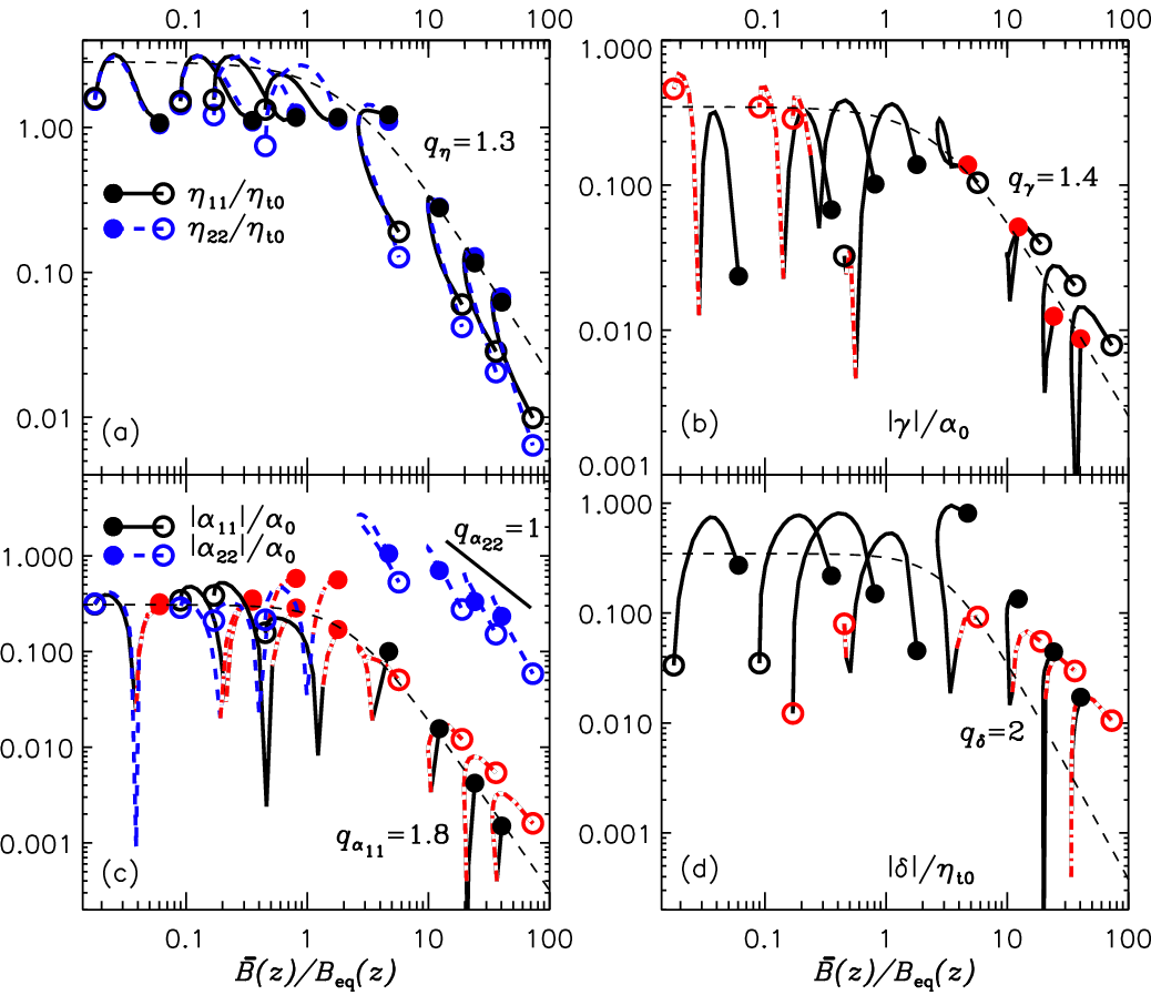
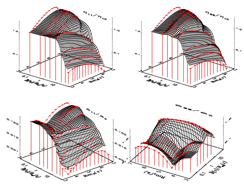
As mentioned above, for the inhomogeneous turbulence in convection we must take into account that . Therefore we show in Figure 12 for Set CR1 (cf. Figure 11), how the transport coefficients are quenched with the local . For comparison, the fit to the averaged quantities from (32) is shown by the dashed lines. A more appropriate representation is obtained by considering the turbulent transport coefficients as functions of both the local and , as they should also depend on the intrinsic (unquenched) local strength of the turbulence. This view is provided in Figure 13 where the arguments in the plane were formed by taking both quantities from the same set of positions within the convection zone for eight different values of . The shown surface was then obtained by linear interpolation over a Delaunay triangulation of the irregularly spaced arguments. In we see for fixed the common power-law quenching behavior, while the dependence on for fixed grows until saturation for small , but falling beyond. shows a similar power-law behavior with for fixed . However, the dependence on is non-monotonic for with a minimum between and 6. As already indicated by Figure 11, the behavior of is different in that, it is first growing with reaching a maximum at for all values of . As a remarkable feature we see a deeply cut valley with respect to with its floor at , ending rather abruptly with a step at . On it and beyond, the dependence is weak with a flat maximum. It remains open, whether the transport coefficients are really local functions of the two quantities employed, or whether there is also a generic dependence on the local mean current density. In addition, non-locality of turbulent transport has been ignored throughout, which is only permissible at large enough scale separation; see [73]. An attempt to fit to a simple ansatz was not satisfactory. Note that the dependences on and were entangled in the result of [8] as there , being dynamo generated, could not be varied independently of .

In another set of simulations, the external field is applied along the vertical direction, see Set CR1Bz in Table 1. Figure 14 shows the dependences of on the external field. We see that is very close to , but now both are quenched with the exponent , which is smaller than the one of for horizontal external field, see Set CR1. Unlike in that case, shows no “anti-quenching”, cf. Figure 11. For and , the quenching exponents are equal to those for the horizontal field case, but for we get instead of 2. To confirm these results, we have repeated the simulations at higher Ra and and find similar results; see Set CR3Bz in Table 1.


IV.3.3 Turbulent pumping for uniform test fields
According to analytic SOCA theory, developed for uniform (or linear) mean fields, turbulent pumping is related to the inhomogeneity of the turbulence through [56]
| (35) |
Hence we now employ TFZ with uniform test fields () in the sets CR6 and CR7 having horizontal imposed field, see Table 1. Figure 15 shows the profiles of for different values of together with those of where has been set to the ( dependent) mixing-length estimate . Comparison reveals that for there is sign agreement of and only close to the bottom of the convection zone. However, already at the signs match rather well and do so perfectly at . The lack of quantitative agreement in the last two cases can most likely be assigned to the crude estimate of . In the unquenched case, by contrast, no complete agreement can be expected since SOCA is no longer reliable at . At this value we are surely beyond the validity range of SOCA, whereas the quenched values of approach it again. For , we see that is strongly quenched, in particular in the upper two thirds of the convective region. A comparison with Figure 8 confirms the strong sensitivity of – even in sign – with respect to the test-field wavenumber, noticed already in [41]. Only for the highest there is some agreement of the profiles for and .
V. Consequences for mean-field dynamos
One of the ultimate goals of our work is the application of the numerically obtained quenching functions to mean-field dynamos that can be validated by comparison against turbulence simulations and that can perhaps eventually be extrapolated to solar and stellar regimes. One of our striking results which might have consequences when applied to mean-field models, is the fact that for isotropically forced turbulence the value of keeps increasing with and exceeds by more than a factor of two when , so turbulent diffusion is enhanced in the direction of the magnetic field relative to that in the perpendicular direction (cf. Equation (5)), but note that is quenched by an order of magnitude and more at such strong . Furthermore, in Equation (5), is negligible compared with , and so are and . Thus the dynamo equation takes the form
| (36) |
where an (anisotropic) effect has been added.
It is important to note that anisotropic diffusion acts here differently from what is sometimes assumed in axisymmetric dynamo models [19, 37, 96, 46, 47, 48]. To clarify this, let us assume that is the toroidal direction and that the toroidal field is dominating, implying and , while and are coordinates in the meridional plane. We can then write the magnetic field as
| (37) |
and, using this in Equation (3) with (4), but , , and neglected, we get [14, cf.]
| (38) | ||||||
| (39) |
where
| (40) | ||||||
| (41) |
With , however, holds, hence the diffusion is actually isotropic. As alluded to above, this is in contrast to previously adopted reasoning by which should be much larger than [19, 37, 96, 46, e.g.,]. We have to stress yet, that the isotropy we found may well be an artefact of the rather specific way of forcing turbulence by transversal waves.
Furthermore, the amount of quenching assumed in some mean-field models is rather large, for example [60] employed a reduction of the magnetic diffusivity by nearly two orders of magnitude in the lower half of the convection zone compared to the mixing length estimate. According to our results, this would require field strengths that exceed the equipartition value correspondingly also by two orders of magnitude. In most of the solar convection zone the equipartition value is around 5000 Gauss [90, see], so the mean field strength required for such strong quenching would have to reach the unlikely order of several Gauss at the bottom.
Although several mean-field dynamo models [5, 39, 30, 25, 49, 65, e.g.,] include turbulent pumping, its quenching is usually ignored. As an exception, Käpylä et al. [39] include quenching of with exponent 2 in a formulation with respect to , which is close to our value of about 2.3.
The question now is to what extent our new results can be used in modelling the mean magnetic field evolution either in turbulence simulations of convectively driven dynamos or even in the Sun. In recent years, simulations have displayed a wealth of different behaviors that are hard to explain with our current knowledge. Examples include the equatorward migration in the simulations of [43], which is only found in the saturated regime of the dynamo and could therefore be connected with quenching, but in ways that are even qualitatively unclear. There are also aspects that might not be possible to capture within the framework of Cartesian geometry such as the extreme concentration of toroidal flux belts or wreaths [12], possibly connected with the dramatic concentration of kinetic helicity toward low latitudes and near the surface; see Figure 1(b) of [43]. One must therefore wait until proper test-field results for azimuthally averaged fields in spherical shells become available.
With these qualifications in mind, we have to content ourselves with statements that we can hope are robust. An example is our finding that the quenching exponents are of the order of unity and the prefactors typically below unity, which suggests that the quenched turbulent transport coefficients should not strongly deviate from their kinematic values if the magnetic field is comparable with the equipartition value. If our results should be employed in a mean-field dynamo model for the Sun, those obtained from convection simulations are the most relevant ones. Therefore, when restricting oneself to the coefficients , , and , one could think about choosing the quenching exponents 3, 2.3, and 2.3, respectively, in expressions of the form (32), providing a somewhat stronger quenching than obtained with the usually adopted exponent 2. However, given that dynamo fields are non-uniform, more elaborated models for the dependence of the transport coefficients on both the local and the local , perhaps even also including a dependence on the local , need to be developed.
VI. Conclusions
We have measured the quenching of the turbulent transport coefficients appearing in the mean-field dynamo equation, in particular , , , , and , by test-field methods. For this, we have considered three different background flows on which uniform external magnetic fields with various directions were imposed. This is of course quite different from the real situation where quenching occurs due to dynamo-generated mean fields; see [8] for a measurement of and at large values of in such a case. Another aspect to keep in mind is that the magnetic and fluid Reynolds numbers of our simulations are far too small in comparison with astrophysical situations. Extrapolation to is feasible once an asymptotic regime is detected, but we emphasize that, in agreement with the results of [8], our maximum value of is not yet sufficient. Nevertheless, the obtained results indicate clear trends that may well apply to more realistic settings and parameter regimes.
In the setup with Roberts I forcing, we have found as a striking property of the quenching behavior its dependence on whether one normalizes the external field with the actual or the original (unquenched) value of the equipartition field strength, or , respectively. In the former case, the quenching exponent for turbulent diffusivity and effect is significantly smaller and closer to that found for forced turbulence and convection (around 1.3). In the latter case, on the other hand, we recover the exponent , found earlier for quenching in the Roberts I flow [72]. Somewhat surprisingly, we find the quenched and to be still isotropic in the plane, in contrast to that paper. However, it is now clear that this is a consequence of their use of a simplified momentum equation and that the obtained isotropy is physically sensible.
For isotropically forced turbulence, the differences between the two normalizations of are not so large and the exponent based on is only around , which is higher than what has been found analytically in Kitchatinov et al. [52] and Rogachevskii & Kleeorin [77], while the exponent based on is around , which is similar to Gressel et al. [29].
Finally we have considered rotating stratified convection. Along with and , we have studied turbulent pumping () and the effect (). We find that and show similar quenching dependences on (with quenching exponent ), while is about 2 for and . However, when is normalized with the exponent becomes , which is agreement with Rüdiger & Kitchatinov [84]. In non-rotating convection, the quenching of and is only slightly weaker compared to the rotating case.
We have not studied the simultaneous quenching of turbulent transport by magnetic field and rotation which is particularly important in rapidly rotating stars. Furthermore, we have not yet applied TFA for convection, which is a subject of our ongoing work. It is unclear, however, how useful it would be to consider quenching with this method, because only one preferred direction is possible. More general methods would be needed in the presence of a strong horizontal magnetic field.
Appendix A Quenching for a single wave flow
Assume the forcing in Equation (8) to be a single transverse (frozen) wave with time-dependent amplitude,
| (A1) |
Then, in the absence of
| (A2) |
is an exact solution of equations (6) and (8) for arbitrary Re as, being a transverse wave, it obeys , and . Further
| (A3) |
is an exact solution of the first-order induction equation with horizontal for arbitrary , again as a consequence of transversality and solenoidality of . Likewise
| (A4) |
is an approximate solution of the second order momentum equation as long as , thus . As (with a time-dependent factor) the argument continues to hold in arbitrary orders in . would even hold for the less restricting condition that only the non-constant part of needs to be negligible. We conclude that the imposed field does not change the geometry of the flow, but only its amplitude. Considering an ensemble of such flows with randomly chosen and , the transport coefficients obtained by ensemble averaging would have to be isotropic, even when quenched, as long as the density remains close to uniform.
References
- [1] Blackman, E. G., & Brandenburg, A. 2002, ApJ, 579, 359
- [2] Braginsky, S. I. 1964, Geomagn. Aeron., 4, 572
- [3] Brandenburg, A. 2001, ApJ, 550, 824
- [4] Brandenburg, A., Jennings, R. L., Nordlund, Å., Rieutord, M., Stein, R. F., & Tuominen, I. 1996, J. Fluid Mech., 306, 325
- [5] Brandenburg, A. Moss, D., & Tuominen, I. 1992, ASP Conf. Ser. (ASP: San Francisco), 27, 536.
- [6] Brandenburg, A., Nordlund, Å., Pulkkinen, P., Stein, R. F., & Tuominen, I. 1990, A&A, 232, 277
- [7] Brandenburg, A., Rädler, K.-H., & Kemel, K. 2012, A&A, 539, A35
- [8] Brandenburg, A., Rädler, K.-H., Rheinhardt, M., & Subramanian, K. 2008a, ApJ, 687, L49
- [9] Brandenburg, A., Rädler, K.-H., Rheinhardt, M., & Käpylä, P. J. 2008b, ApJ, 676, 740
- [10] Brandenburg, A., Gressel, O., Käpylä, P. J., Kleeorin, N., Mantere, M. J., & Rogachevskii, I. 2013, ApJ, 762, 127
- [11] Brandenburg, A., Rädler, K.-H., & Schrinner, M. 2008c, A&A, 482, 739
- [12] Brown, B. P., Browning, M. K., Brun, A. S., Miesch, M. S., & Toomre, J. 2010, ApJ, 711, 424
- [13] Brun, A. S., Miesch, M. S., & Toomre, J. 2004, ApJ, 614, 1073
- [14] Bykov, A. M., Brandenburg, A., Malkov, M. A., & Osipov, S. M. 2013, Spa. Sci. Rev., 178, 201
- [15] Cattaneo, F., & Vainshtein, S. I. 1991, ApJ, 376, L21
- [16] Cattaneo, F., & Hughes, D. W. 1996, Phys. Rev. E, 54, R4532
- [17] Charbonneau, P. 2010, Liv. Rev. Sol. Phys., 7, 3
- [18] Choudhuri, A. R., & Gilman, P. A. 1987, ApJ, 316, 788
- [19] Chatterjee, P., Nandy, D., & Choudhuri, A. R. 2004, A&A, 427, 1019
- [20] Choudhuri, A. R., & Karak, B. B. 2009, RAA, 9, 953
- [21] Choudhuri, A. R., & Karak, B. B. 2012, Phys. Rev. Lett., 109, 171103
- [22] Covas, E., Tavakol, R., Tworkowski., A., & Brandenburg, A. 1998, A&A, 329, 350
- [23] D’Silva, S., & Choudhuri, A. R. 1993, A&A, 272, 621
- [24] Del Sordo, F., Guerrero, G., & Brandenburg, A. 2013, MNRAS, 429, 1686
- [25] Do Cao, O., & Brun, A. S. 2012, Astron. Nachr., 332, 907.
- [26] Gilman, P. A. 1983, ApJS, 53, 243
- [27] Gilman, P. A. & Miller, J. 1981, ApJ, 46, 211
- [28] Glatzmaier, G. A. 1985, ApJ, 291, 300
- [29] Gressel, O., Bendre, A. & Elstner, D. 2013, MNRAS, 429, 967
- [30] Guerrero, G., & de Gouveia Dal Pino, E. M. 2008, ApJ, 485, 267
- [31] Guerrero, G. Dikpati, M. & de Gouveia Dal Pino, E. M. 2009, ApJ, 701, 725
- [32] Heinemann, T., McWilliams, J. C., & Schekochihin, A. A. 2011, Phys. Rev. Lett., 107, 255004
- [33] Hubbard, A., & Brandenburg, A. 2009, ApJ, 706, 712
- [34] Hubbard, A., Del Sordo, F., Käpylä, P. J., & Brandenburg, A. 2009, MNRAS, 398, 1891
- [35] Hurlburt, N. E., Toomre, J., & Massaguer, J. M. 1986, ApJ, 311, 563
- [36] Jepps, S. A. 1975, J. Fluid Mech., 67, 625
- [37] Jiang, J., Chatterjee, P., & Choudhuri, A. R. 2007, MNRAS, 381, 1527
- [38] Käpylä, P. J., & Brandenburg, A. 2009, ApJ, 699, 1059
- [39] Käpylä, P. J., Korpi, M. J., & Tuominen, I. 2006, Astron. Nachr., 327, 884
- [40] Käpylä, P. J., Korpi, M. J., & Brandenburg, A. 2008, A&A, 491, 353
- [41] Käpylä, P. J., Korpi, M. J., & Brandenburg, A. 2009a, A&A, 500, 633
- [42] Käpylä, P. J., Korpi, M. J., & Brandenburg, A. 2009b, ApJ, 697, 1153
- [43] Käpylä, P. J.,Mantere, M. J & Brandenburg, A. 2012, ApJ, 755, 22
- [44] Käpylä, P. J., Mantere, M. J., Cole, E., Warnecke, J., & Brandenburg, A. 2013, ApJ, 778, 41
- [45] Karak, B. B. 2010, ApJ, 724, 1021
- [46] Karak, B. B., & Choudhuri, A. R. 2011, MNRAS, 410, 1503
- [47] Karak, B. B., & Choudhuri, A. R. 2012, Sol. Phys., 278, 137
- [48] Karak B. B., & Choudhuri, A. R. 2013, RAA, 13, 1339
- [49] Karak B. B, & Nandy D. 2012, ApJ, 761, L13
- [50] Karak B. B, & Käpylä, P. J., Käpylä, M. J & Brandenburg, A. A&A, 2014, arXiv:1407.0984
- [51] Kitchatinov, L. L., & Pipin, V. V. 1993, A&A, 274, 647
- [52] Kitchatinov, L. L., Pipin, V. V. & Rüdiger, G. 1994, Astron. Nachr., 315, 157
- [53] Kleeorin, N. I., & Ruzmaikin, A. A. 1982, Magnetohydrodynamics, 18, 116
- [54] Kleeorin, N., Moss, D., Rogachevskii, I., & Sokoloff, D. 2000, A&A, 361, L5
- [55] Köhler, H. 1973, A&A, 25, 467
- [56] Krause, F., & Rädler, K.-H., 1980, Mean-Field Magnetohydrodynamics and Dynamo Theory, Akademie-Verlag Berlin and Pergamon Press Cambridge
- [57] Mitra, D., & Brandenburg, A. 2012, MNRAS, 420, 2170
- [58] Mitra, D., Käpylä, P. J., Tavakol, R., & Brandenburg, A. 2009, A&A, 495, 1
- [59] Moffatt, H. K. 1972, J. Fluid Mech., 53, 385
- [60] Muñoz-Jaramillo, A., Nandy, D., & Martens, P. C. H. 2011, ApJ, 727, L23
- [61] Ossendrijver, M., Stix, M., & Brandenburg, A. 2001, A&A, 376, 713
- [62] Parker, E. N. 1955, ApJ, 122, 293
- [63] Pipin, V. V., & Seehafer, N. 2009, A&A, 493, 819
- [64] Pipin, V. V., & Kosovichev, A. G. 2011, ApJ, 727, L45
- [65] Pipin, V. V., & Kosovichev, A. G. 2014, ApJ, 785, 49
- [66] Pouquet, A., Frisch, U., & Léorat, J. 1976, J. Fluid Mech., 77, 321
- [67] Racine, E., Charbonneau, P., Ghizaru, M., Bouchat, A. & Smolarkiewicz, P. K. 2011, ApJ, 735, 46
- [68] Rädler, K.-H. 2014, Astron. Nachr., 335, 459
- [69] Rädler, K.-H., Rheinhardt, M., Apstein, E., & Fuchs, H., Magnetohydrodynamics 38, 39, 2002a
- [70] Rädler, K.-H., Rheinhardt, M., Apstein, E., & Fuchs, H., Nonlinear Processes in Geophysics 9, 171, 2002b
- [71] Rempel, M. 2006, ApJ, 647, 662
- [72] Rheinhardt, R., & Brandenburg, A. 2010, A&A, 520, 28
- [73] Rheinhardt, M., & Brandenburg, A. 2012, Astron. Nachr., 333, 71
- [74] Rheinhardt, M., Devlen, E., Rädler, K.-H., & Brandenburg, A. 2014, MNRAS, 441, 116
- [75] Roberts, G. O. 1972, Phil. Trans. Roy. Soc., A 271, 411
- [76] Roberts, P. H., & Soward, A. M. 1975, Astron. Nachr., 296, 49
- [77] Rogachevskii, I. & Kleeorin, N. 2000, Phys. Rev. E, 61, 5202
- [78] Rogachevskii, I. & Kleeorin, N. 2001, Phys. Rev. E, 64, 056307
- [79] Rogachevskii, I. & Kleeorin, N. 2003, Phys. Rev. E, 68, 036301
- [80] Rogachevskii, I. & Kleeorin, N. 2006, Geophys. Astrophys. Fluid Dyn., 100, 243
- [81] Rogachevskii, I., Kleeorin, N., Brandenburg, A., & Eichler, D. 2012, ApJ, 753, 6
- [82] Rüdiger, G. 1974, Astron. Nachr., 295, 275
- [83] Rüdiger, G. & Brandenburg, A. 1995, A&A, 296, 557
- [84] Rüdiger, G., & Kitchatinov, L. L. 1993, Astron. Nachr., 269, 581
- [85] Rüdiger, G., & Kitchatinov, L. L. 2000, Astron. Nachr., 321, 75
- [86] Rüdiger, G., Kitchatinov, L. L., Küker, M., & Schultz, M. 1994, Geophys. Astrophys. Fluid Dyn., 78, 247
- [87] Schrinner, M., Rädler, K.-H., Schmitt, D., Rheinhardt, M., Christensen, U. 2005, Astron. Nachr., 326, 245
- [88] Schrinner, M., Rädler, K.-H., Schmitt, D., Rheinhardt, M., Christensen, U. R. 2007, Geophys. Astrophys. Fluid Dyn., 101, 81
- [89] Steenbeck, M., Krause, F., & Rädler, K.-H. 1966, Z. Naturforsch., 21a, 369
- [90] Stix, M. 2002, The Sun: An introduction (Springer-Verlag, Berlin)
- [91] Sur, S., Subramanian, K. & Brandenburg, A. 2007, MNRAS, 376, 1238
- [92] Sur, S., Brandenburg, A., & Subramanian, K. 2008, MNRAS, 385, L15
- [93] Vainshtein, S. I., & Cattaneo, F. 1992, ApJ, 393, 165
- [94] Vishniac, E. T., & Brandenburg, A. 1997, ApJ, 475, 263
- [95] Weber, M. Fan, Y. Miesch, M. S. 2011, ApJ, 741, 11
- [96] Yeates, A. R., Nandy, D., & Mackay, D. H. 2008, ApJ, 673, 544
- [97] Yousef, T. A., Brandenburg, A., & Rüdiger, G. 2003, A&A, 411, 321
$Header: /var/cvs/brandenb/tex/karak/aniso/paper.tex,v 1.378 2014/08/20 17:56:08 rei Exp $