Extracting information from S-curves of language change

Fakhteh Ghanbarnejad Thanks: Both authors contributed equally to this work. Affiliation: Max Planck Institute for the Physics of Complex Systems, Dresden, Germany Email: fakhteh,gerlach,jmiotto,edugalt@pks.mpg.de Martin Gerlach Thanks: Both authors contributed equally to this work. Affiliation: Max Planck Institute for the Physics of Complex Systems, Dresden, Germany José M. Miotto Affiliation: Max Planck Institute for the Physics of Complex Systems, Dresden, Germany Eduardo G. Altmann Affiliation: Max Planck Institute for the Physics of Complex Systems, Dresden, Germany

Abstract

It is well accepted that adoption of innovations are described by S-curves (slow start, accelerating period, and slow end). In this paper, we analyze how much information on the dynamics of innovation spreading can be obtained from a quantitative description of S-curves. We focus on the adoption of linguistic innovations for which detailed databases of written texts from the last 200 years allow for an unprecedented statistical precision. Combining data analysis with simulations of simple models (e.g., the Bass dynamics on complex networks) we identify signatures of endogenous and exogenous factors in the S-curves of adoption. We propose a measure to quantify the strength of these factors and three different methods to estimate it from S-curves. We obtain cases in which the exogenous factors are dominant (in the adoption of German orthographic reforms and of one irregular verb) and cases in which endogenous factors are dominant (in the adoption of conventions for romanization of Russian names and in the regularization of most studied verbs). These results show that the shape of S-curve is not universal and contains information on the adoption mechanism. (published at "J. R. Soc. Interface, vol. 11, no. 101, (2014) 1044"; DOI: http://dx.doi.org/10.1098/rsif.2014.1044)

I Introduction

The term S-curve often amounts to the qualitative observation that the change starts slowly, accelerates, and ends slowly. Linguists generally accept that “the progress of language change through a community follows a lawful course, an S-curve from minority to majority to totality.” [1], see Ref. [2] for a recent survey of examples in different linguistic domains. Quantitative analysis are rare and extremely limited by the quality of the linguistic data, which in the best cases have “up to a dozen points for a single change” [2]. Going beyond qualitative observation is essential to address questions like:

Figure 1: (color online) Examples of linguistic changes showing different adoption curves. We estimate the fraction of adopters

\rho(t)

by the relative frequency as

\rho(t)=\sum_{w}n^{w}_{1}/\sum_{w}\sum_{q}n^{w}_{q}

, where

n^{w}_{q}

is the total number of occurrences (tokens) of variant

q

for the word

w

at year

t

. (a) The orthography of German words that changed to “ss” (

q=1

) from “ß” (

q=2

) in the orthographic reform of 1996 (many words changed from “ss” to “ß” in the 1901 reform). (b) The transliteration of Russian names ending with the letter “в” when written in English (Latin alphabet), changed to an ending in “v” (

q=1

) from endings in “ff” (

q=2

) or “w” (

q=3

) (e.g.,

w=

“Саратов” is nowadays almost unanimously written as “Saratov”, but it used to be written also as “Saratoff” or “Saratow”). (c) The past form of the verb spill changed to its regular form “spilled” (

q=1

) from the irregular form “spilt” (

q=2

). The light curve shows the fit of Eq. (2). The estimated parameters

a

and

b

are (a)

\hat{a}=0.218,\hat{b}=0.000

in 1901, and

\hat{a}=0.229

\hat{b}=0.000

in 1996; (b)

\hat{a}=0.000

\hat{b}=0.099

; and (c)

\hat{a}=0.001

\hat{b}=0.030

. The corpus is the Google-ngram [3, 4] plotted in the minimum (yearly) resolution, see supplementary material (SM) Sec. I for details on the data and Sec. IIIB for details on the fit.

(i)

Are all changes following S-curves?
(ii)

Are all S-curves the same (e.g., universal after proper re-scaling)?
(iii)

How much information on the process of change can be extracted from S-curves?
(iv)

Based on S-curves, can we identify signatures of endogenous and exogenous factors responsible for the change?

Large records of written text available for investigation provide a new opportunity to quantitatively study these questions in language change [3, 4]. In Fig. 1 we show the adoption curves of three linguistic innovations for which words competing for the same meaning can be identified. Our methodology is not restricted to such simple examples of vocabulary replacement and can be applied to other examples of language change and S-curves more generally. Here we restrict ourselves to data of aggregated (macroscopic) S-curves because only very rarely one has access to detailed data at the individual (microscopic) level, see, e.g., Ref. [5] for an exception.

Data alone is not enough to address the questions listed above, it is also essential to consider mechanistic models responsible for the change [6, 7, 8, 2, 9]. Dynamical processes in language can also be described from the more general perspectives of evolutionary processes [2, 6, 10] and complex systems [11, 12, 13]. In this framework, the adoption of new words can be seen as the adoption of innovations [14, 15, 16, 17, 18, 9]. One of the most general and popular models of innovation adoption showing S-curves is the Bass model [16, 17]. In its simplest case, it considers a homogeneous population and prescribes that the fraction of adopters ( $\rho$ ) increases because those that have not adopted yet ( $1-\rho$ ) meet adopters (at a rate $b$ ) and are subject to an external force (at a rate $a$ ). The adoption is thus described by

\frac{d\rho(t)}{dt}=(a+b\rho(t))(1-\rho(t)).

(1)

The solution (considering $\rho(t_{0})=\rho_{0}$ and $\rho(\infty)=1$ ) is

\rho(t)=\frac{a(1-\rho_{0})-(a+b\rho_{0})e^{(a+b)(t-t_{0})}}{-b(1-\rho_{0})-(a+b\rho_{0})e^{(a+b)(t-t_{0})}}.

(2)

It contains as limiting cases a symmetric S-curve (for $a=0$ ) and an exponential relaxation (for $b=0$ ). The fitting of Eq. (2) to the data in Fig. 1 leads to very different $a$ and $b$ in the three different examples, strongly suggesting that the S-curves are not universal and contain information on the adoption process. For instance, orthographic reforms are known to be exogenously driven (by language academies) in agreement with $b=0$ obtained from the fit in panel (a).

In this paper we investigate the shape and significance of S-curves in models of adoption of innovations and in data of language change. In particular, we estimate the contribution of endogenous and exogenous factors in S-curves, a popular question which has been addressed in complex systems more generally [19, 20, 21, 22]. The different values of $a$ and $b$ in Eq. (1) are an insufficient quantification, e.g., because they fail to indicate which factor is stronger. Here we introduce a definition for the relevance of different factors in a change. We then show how this quantity can be exactly computed in different models and propose three different methods to estimate it from the time series of $\rho(t)$ . We compare the accuracy of the methods using simulations of different network models and we apply the methods to linguistic changes. We obtain that the exogenous factors are responsible for the change in the German orthographic reforms, but it plays a minor role in the case of romanized Russian names and in most of the studied English verbs which are moving towards regularization.

II Theoretical Framework

Consider that $i=1,\dotsc,N\rightarrow\infty$ identical agents (assumption 1) adopt an innovation. The central quantity of interest for us here is $\rho(t)=N(t)/N$ , the fraction of adopters at time $t$ . We assume that $\rho(t)$ is monotonically increasing from $\rho_{0}\equiv\rho(0)\approx 0$ to $\rho(\infty)=1$ and agents after adopting the innovation do not change back to non-adopted status (assumption 2).

II.1 Endogenous and Exogenous Factors

In theories of language and cultural change, the importance of different factors is a topic of major relevance, e.g., Labov’s internal and external factors [1] and Boyd and Richerson’s different types of biases in cultural transmission [10]. The first question we address is how to measure the contribution of different factors to the change. To the best of our knowledge, no general answer to this question has been proposed and computed in adoption models. As a representative case, we divide factors as endogenous and exogenous to the population. Mass media and decisions from language academies count as exogenous factors while grassroots spreading as an endogenous factor. In our simplified classification, Labov’s internal (external) factors (to properties of the language [1]) are counted by us as exogenous (endogenous), while Boyd and Richerson’s [10] direct bias count as exogenous whereas the indirect bias and frequency-dependent bias count as endogenous.

Our proposal is to quantify the importance of a factor $j$ as the number of agents that adopted the innovation because of $j$ . More formally, let $g_{i}(t)$ be the adoption probability at time $t$ for agent $i$ (who is in the non-adopted status). We assume that $g_{i}$ can be decomposed in contributions of the different factors $j$ as $g_{i}(t)=\sum_{j}g_{i}^{j}(t)$ , where $g_{i}^{j}(t)$ is the adoption probability of agent $i$ at time $t$ because of factor $j$ . If $t_{i}^{*}$ denotes the time agent $i$ adopts the innovation, $g_{i}^{j}(t^{*}_{i})/g_{i}(t^{*}_{i})$ quantifies the contribution of factor $j$ to the adoption of agent $i$ (the adoption does not explicitly depends on $t<t^{*}$ and therefore values of $g_{i}^{j}(t)$ for $t<t^{*}$ are only relevant in the extent that they influence $g_{i}^{j}(t=t^{*})$ ). In principle, the factor $g_{i}^{j}(t^{*}_{i})/g_{i}(t^{*}_{i})$ can be obtained empirically by asking recent adopters for their reasons for changing, e.g., for j=exogenous (endogenous) one could ask: How much advertisement (peer pressure) affected your decision?. We define the normalized quantification of the change in the whole population due to factor $j$ as an average over all agents

G^{j}=\frac{1}{N}\sum_{i=1}^{N}\frac{g_{i}^{j}(t^{*}_{i})}{g_{i}(t^{*}_{i})}.

(3)

In order to show the significance of definition (3), and how it can be applied in practice, we discuss how $g^{j}_{i}$ and $G^{j}$ can be considered in different models. Endogenous (endo) factors happen due to the interaction of an agent with other agents (internal to the population). They are therefore expected to become more relevant as the adoption progress (for increasing $\rho$ ). Exogenous factors (exo), on the other hand, are related to a source of information (external to the population) which has no dependence on $\rho$ or time (assumption 3). For simplicity, we report $G\equiv G^{\text{exo}}$ (since $G^{\text{endo}}=1-G^{\text{exo}}$ ).

II.2 Population dynamics models

Consider as a more general form of Eq. (1)

\dot{\rho}(t)\equiv\dfrac{d\rho(t)}{dt}=g(\rho(t))(1-\rho(t)),

(4)

where $g(\rho(t))$ is the probability that the population of non-adopters $(1-\rho(t))$ switches from non-adopted status (0) to adopted status (1) at a given density of $\rho$ . In epidemiology $g(\rho)$ is known as force of infection [23]. Since agents are identical (assumption 1) and $\rho(t)$ is invertible (assumption 2), we can associate $g_{i}^{j}(t_{i}^{*})$ with $g^{j}(\rho)$ and $g_{i}(t_{i}^{*})$ with $g(\rho)$ . Introducing $g(\rho(t))$ from Eq. (4) in the continuous time extension of definition (3) we obtain:

G^{j}\equiv\int_{0}^{1}\frac{g^{j}(\rho)}{g(\rho)}d\rho=\int_{0}^{1}g^{j}(\rho)\frac{1-\rho}{\dot{\rho}}d\rho=\int_{0}^{\infty}\frac{g^{j}(t)}{g(t)}\dot{\rho}(t)dt.

(5)

This equation shows that the strength of factor $j$ is obtained by averaging its normalized strength $g^{j}(\rho)/g(\rho)$ over the whole population or, equivalently, over time (considering the rate of adoption $\dot{\rho}(t)$ ).

When only exogenous and endogenous factors are taken into consideration, $g(\rho)=g^{exo}+g^{\text{endo}}$ in Eq. (4). Here, assumption 3 mentioned above corresponds to consider that the adoption happens much faster than the changes in the exogenous factors so that it can be considered independent of time. Therefore $g^{\text{exo}}=g(\rho=0)$ . Any change of $g$ with $\rho$ is an endogenous factor and $g^{\text{endo}}(\rho)$ increases with $\rho$ because the pressure for adoption increases with the number of adopters.

For the case of the Bass model defined in Eq. (1), $g(\rho)=a+b\rho,g^{endo}=a,g^{exo}=b\rho$ and from Eq. (5) we obtain

\displaystyle G\equiv G^{\text{exo}}=\frac{a}{b}\log_{e}(\frac{a+b}{a}).

(6)

The correspondence of $a$ and $b\rho$ to exogenous (innovators) and endogenous (imitators) is a basic ingredient of the Bass model [16] ¹¹ 1 In our simple model, all agents are identical. The first adopters (innovators) are determined stochastically by the exogenous factor $a$ , while agents adopting at the end of the S-curve (imitators) are more susceptible to the endogenous factor $b\rho$ .. However, it is only through Eq. (6) that the importance of these factors to the change can be properly quantified. For instance, the case $a=b$ suggests equal contribution of the factors, but Eq. (6) leads to $G=\log_{e}2\approx 0.69>0.5$ and therefore shows that the exogenous factors dominate (are responsible for a larger number of adoptions than the endogenous factors). This new insight on the interpretation of the classical Bass model illustrates the significance of Eq. (3) and our general approach to quantify the contribution of factors.

II.3 Binary state models on networks

Another well-studied class of models inside our framework considers agents characterized by a binary variable $s=\{0,1\}$ connected to each other through a network. We focus on models with a monotone dynamics (assumption 2), such as the Bass, Voter, and Susceptible Infected models, which are defined by the probability $F_{k,m}$ of switching from $0$ to $1$ given that the agent has $k$ neighbours and $m$ neighbours in state $1$ [24]. The one dimensional population dynamics model in Eq. (4) can be retrieved for simple networks (e.g., fully connected or fixed degree). In the general case, we use the framework of approximate master equations (AME) [25, 26] (see SM. II), which describes the stochastic binary dynamics in a random network with a given degree distribution $P_{k}$ . Assuming as before (assumption 3) that the exogenous contribution is given by transitions that occur when no neighbour is infected, i.e. $g^{\mathrm{\text{exo}}}\left(k,m\right)=F_{k,0}$ , we obtain the exogenous contribution as (see SM. IIB):

G=\sum_{k}P_{k}\sum_{m=0}^{k}\int_{0}^{\infty}s_{k,m}F_{k,0}\mathrm{d}t,

(7)

where $s_{k,m}=s_{k,m}(t)$ is the fraction of agents of the $k,m$ class in state $0$ .

Figure 2: Application of time-series estimations to surrogate data. The Bass (a,b) and threshold (c,d) dynamics with parameters

a=0.1

and

b=0.5

were numerically solved in the AME framework for scale free networks (with degree distribution

P(k)\sim k^{-\gamma}

with

\gamma\approx 2.47

for

k\in[2,50]

such that

\langle k\rangle=4

). (a,c) Adoption curve

\rho(t)

(fraction of adopted agents over time). (b,d) Numerical estimate of

g(\rho)

, obtained from

\rho(t)

by inverting Eq. (4). Dashed curves correspond to the fit of Eq. (2) to

\rho(t)

. Estimations of

G

correspond to the area between the horizontal gray line (

g(\rho)=\hat{a}

) and the solid (

{\tilde{G}}

) or dashed (

\hat{G}

) curves in (b,d). Results: Bass

G=0.397,L=0.999,\hat{G}=0.415,\tilde{G}=0.400

; Threshold

G=0.347,L=0.988,\hat{G}=0.314,\tilde{G}=0.352

Refer to caption — Figure 3: (color online) Strength of endogenous factors $G$ in the Bass [Eq. (8), panels a,b,c] and threshold [Eq. (9), panels d,e,f] models for different parameters $a$ and $b$ . The dashed lines correspond to values of $a,b$ for which $G=1/2$ (red), $G=1/3$ (black below red), and $G=2/3$ (black above red), computed from Eq. (7). The different panels show the estimations based on $L$ (a,d), $\hat{G}$ (b,e), and $\tilde{G}$ (c,f). Solid lines indicate values of $a,b$ for which values $1/2,1/3,$ and $2/3$ were obtained and should be compared to the corresponding dashed lines. The color code indicates the relative errors between the true value $G$ and the estimated values $\hat{G}$ (b,e) and $\tilde{G}$ (c,f). The model dynamics was simulated for scale-free networks with the same parameters as in Fig. 2.

III Time series estimators

In reality one usually has no access to information on individual agents and only the aggregated curve $\rho(t)$ is available. This means that $G$ can not be estimated by Eqs. (3) or (7). Here we propose and critically discuss the accuracy of three different methods to estimate $G$ from the S-curve $\rho(t)$ obtained from either empirical or surrogate data. All methods are inspired by the simple population model discussed above, but can be expected to hold also in more general cases. Below we summarize the main idea of the three methods, details on the implementation appear in SM. III.

Method 1, fit of S- and exponential curves: We fit Eq. (2) by minimizing the Least-Square error with respect to the observed timeseries in the two limiting cases: (i) $a=0$ , symmetric S-curve (endogenous factors only) and (ii) $b=0$ , exponential curve (exogenous factors only). Assuming normally distributed errors (which generically vary in time) we calculate the likelihood of the data given each model [27]. The normalized likelihood ratio $L$ of the two models indicates which curve provides a better description of the data [28]. The critical assumption in this method (to be tested below) is to consider the value of $L$ as an indication of the predominance of the corresponding factor, i.e $L>0.5$ indicates stronger exogenous factors $(G>0.5)$ and $L<0.5$ stronger endogenous factors $(G<0.5)$ . This method does not allow for an estimation of $G$ , but it provides an answer to the question of the most relevant factors. The two simple one-parameter curves are unlikely to precisely describe many real adoption curves $\rho(t)$ . However, we expect that they will distinguish between cases showing a rather fast/abrupt start at $t_{0}$ (as in the exponential/exogenous case) from the ones showing a slow/smooth start (as in the S-curve/endogenous case). For this distinction, the $t\gtrapprox 0$ is the crucial part of the $\rho(t)$ curve because for $t\rightarrow\infty$ the symmetric S-curve approaches $\rho=1$ also exponentially.

Method 2, fit of generalized S-curve: We fit Eq. (2) by minimizing the Least-Square error with respect to the timeseries and obtain the estimated parameters $\hat{a}$ and $\hat{b}$ . By inserting these parameters in Eq. (6) we compute $\hat{G}$ as an estimation of $G$ .

Method 3, estimation of $g(\rho)$ : We estimate $g(\rho)$ from Eq. (4) by calculating a (discrete) time derivative $\dot{\rho}$ at every point $\rho(t)$ . From a (smoothed) curve of $g(\rho)$ we consider $g(0)$ to be the exogenous factors, write $g^{\text{endo}}=g(\rho)-g(0)$ and obtain an estimation ${\tilde{G}}$ of $G$ from Eq. (5). The advantage of this non-parametric method is that it is not a priory attached to a specific $g(\rho)$ and therefore it is expected to work whenever a population dynamics equation (4) provides a good approximation of the data.

IV Application to network models

Here we investigate time series $\rho(t)$ obtained from simulations of models in which we have access to the microscopic dynamics of agents. Our goal is to measure $G$ on different models and to test the estimators ( $L,\tilde{G},\hat{G}$ ) defined in the previous section. We consider two specific network models in the framework described in Sec. II.3, which are defined fixing the network topology (in our case random scale-free) and the function $F_{k,m}$ (the adoption rate of an agent having $m$ out of $k$ neighbours that already adopted) as [25, 24]:

\text{Bass model: }F_{k,m}=a+b\frac{m}{k},

(8)

\text{Threshold: }F_{k,m}=\begin{cases}a,&m/k<1-b\\ 1,&m/k\geq 1-b\end{cases}.

(9)

In both cases, when no infected neighbor is present ( $m=0$ ), the rate is $F_{k,0}=a$ and therefore the parameter $a$ controls the strength of exogenous factors. Analogously, $b$ controls the increase of $F_{k,m}$ with $m$ and therefore the strength of endogenous factors. Given a network and values of $a$ and $b$ , we obtain numerically both the timeseries $\rho(t)$ (using the AME formalism [25, 26], SM. IIC), and the strength of exogenous factors $G$ from Eq. (7). Typically these models cannot be reduced to a one-dimensional population dynamics model and therefore the estimators $\hat{G}$ and $\tilde{G}$ (based on $\rho(t)$ ) differ from the actual $G$ . As a test of our methods, we compare the exact $G$ to $L$ , $\hat{G}$ and ${\tilde{G}}$ .

In Fig. 2 we apply our time-series analysis to the two models defined above with parameters $a=0.1,b=0.5$ . Method 1 provides $L>0.5$ in both cases, incorrectly identifying that the exogenous factor is stronger. Furthermore, $\tilde{G}$ (Method 3) provides a better estimation of $G$ than $\hat{G}$ (Method 2). This is expected since the estimation $\hat{G}$ is based on a straight line estimation of $g(\rho)$ , $(\hat{a}+\hat{b}\rho)$ , while $\tilde{G}$ admits more general function, see Fig. 2, (b,d). The estimations are better for the Bass model than for the threshold dynamics, consistent with the better agreement between $\rho(t)$ and the fit of Eq. (2) in panel (a) than in panel (c).

In Fig. 3 we repeat the analysis of Fig. 2 varying the parameters $a,b$ in Eqs. (8) and (9), while Eq. (7) gives the true value of $G$ . The parameter space $a,b$ is divided in two regions: one for which the exogenous factors dominate $G>0.5$ (below the red dashed line $G=0.5$ ) and one for which the endogenous factors dominate $G<0.5$ (above the red dashed line $G=0.5$ ). In the Bass dynamics the division between these regions corresponds to a smooth (roughly straight) line. In the threshold model a more intricate curve is obtained, with plateaus on rational values of $b$ reflecting the discretization of the threshold dynamics in Eq. (9) (particularly strong for the large number of agents with few neighbors). A strong indication of the limitations of the $L$ and $\hat{G}$ estimators is that the $L=0.5$ (panel d) and $\hat{G}=0.5$ (panel e) lines show non-monotonic growth in the $a,b$ space. This artifact disappears using the ${\tilde{G}}$ estimator. Regarding the relative errors of the methods 2 and 3 (colour code), the results confirm that $\tilde{G}$ is the best method and provides a surprisingly accurate estimation of $G$ . Comparing the different models, the estimations for Bass are better than for the threshold dynamics (for the same parameters $(a,b)$ ). The minimum errors are obtained for $b\approx 0$ while for $a\approx 0$ maximum errors for both methods are observed.

V Application to data

We now turn to the analysis of empirical data taken from the Google-ngram corpus [3, 4], see Ref. [29] and SM. I. We focus on the three cases reported in Fig. 1:

a. German orthographic reforms: The 1996 orthography reform aimed to simplify the spelling of the German language based on phonetic unification. According to this reform, after a short vocal one should write “ss” instead of “ß”, which predominated since the previous reform in 1901. This rule makes up over $90\%$ of the words changed by the reform [30]. We combine all words affected by this rule to estimate the strength of adoption of the orthographic reform, i.e., $\rho(t)$ is the fraction of word tokens in the list of affected words written with “ss”. Although following the reform was obligatory at schools, strong resistance against it led to debates even in the Federal Constitutional Court of Germany [31]. For example, “six years after the reform, $77\%$ of Germans consider the spelling reform not to be sensible [30]”. These debates show that besides the exogenous pressure of language academies, endogenous factors can be important in this case also, either for or against the change.

b. Russian names: Since the $19$ th century there have been different systems for the romanization of Russian names, i.e. for mapping names from the Cyrillic to the Latin alphabet [32]. These systems can be seen as exogenous factors. Alternatively, imitation from other authors can be considered as endogenous factors. All of the systems suggest a unique mapping from letter “в” to “v” (e.g., Колмогоров to Kolmogorov). Variants to this official romanization system are “ff” or “w” (e.g., Kolmogorow and Kolmogoroff) which were used in different languages such as German and English. Here we study an ensemble of $50$ Russian names ending in either “-ов” or “-eв” that were used often in English (en) and German (de). For each of these two languages, we combine all words (tokens) in order to obtain a single curve $\rho(t)$ measuring the adoption of the “v” convention.

c. Regularization verbs in English: A classical studied case of grammatical changes is regularization of English verbs [33, 34]. From 177 irregular verbs in Old-English, 145 cases survived in Middle English and only 98 are still alive [33]. Irregular verbs coexist with their regular (past tense written by -ed) competitors, even if dictionaries may only present irregular forms [3]. Having an easier grammar rule or a rule aligned with a larger grammatical class are good motivations to use more often regular forms. Other potential exogenous factors which favour works against regularization can be dictionaries and grammars. However, there are also cases of verbs that become irregular [3, 35]. We analyse $10$ verbs that exhibit the largest relative change. In $8$ cases regularization is observed.

Figure 5: (color online) Method 2 is more robust against perturbations than Method 3. Estimation of G in undersampled versions of the timeseries used in Fig. (2) for Bass (left) and threshold (right) dynamics. The true

G

[Eq. (7)] is shown as a dashed line and Methods 2 and 3 are shown by symbols. (a,b) Undersampling in time: achieved by varying the time-resolution

\Delta t

of the timeseries, i.e., we sample

\rho(t)

at times

\rho(t_{0}),\rho(t_{0}+\Delta t),\rho(t_{0}+2\Delta t),\ldots

. Resolution increases for

\Delta t\rightarrow 0

. (c,d) Undersampling of the population

N

. The surrogate time series

\rho(t)

in Fig. 2 assume

N\rightarrow\infty

. We consider time series for which only a finite population

N

is observed. The observed fraction of adopters is determined from

N

independent Bernoulli trials with probability

\rho(t)

. This corresponds to adding noise to each data point

\rho(t)

. Resolution increases for

N\rightarrow\infty

. For each

N

, we plot the average and standard deviation of

G

computed over

1,000

trials.

Besides the linguistic and historical interest in these three cases, there are also two practical reasons for choosing these three simple spelling changes: (i) they provide data with high resolution and frequency; and (ii) they allow for an unambiguous identification of “competing variants”, a difficult problem in language change [36]. The last point allows us to concentrate on the relative word frequency (as defined in the caption of Fig. 1) which we identify with the relative number of adopters $\rho(t)$ in the models of previous sections. The advantage of investigating relative frequencies, instead of the absolute frequency of usage of one specific variation, is that they are not affected by absolute changes in the usage of the word.

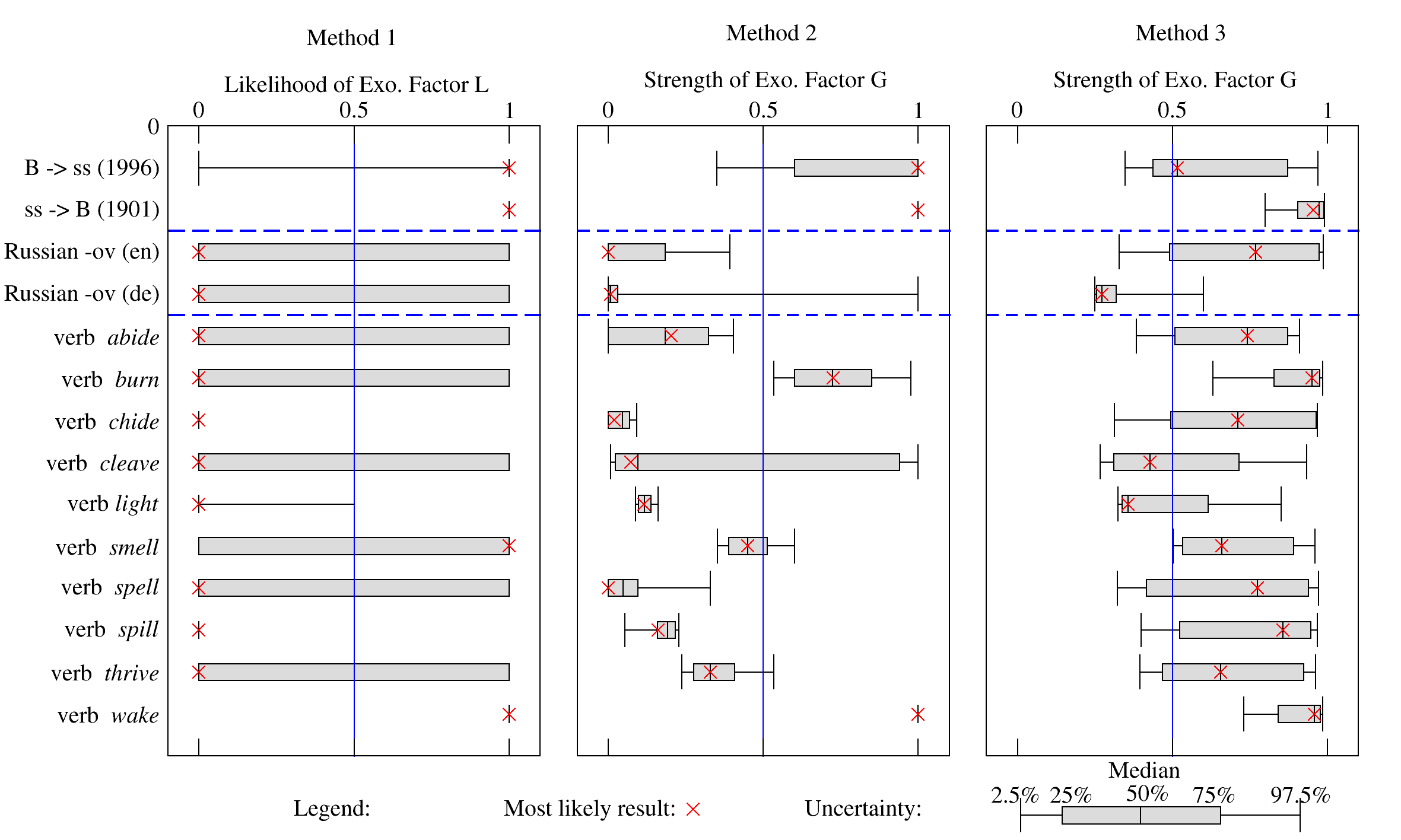
Fig. 4 shows estimations of the strength of exogenous factors G (using the methods of Sec. III) in the three examples of linguistic change described above. In line with the definition proposed in Sec. II, $G$ is interpreted as the fraction of adoptions because of exogenous factors. Besides the most-likely estimation obtained for the complete datasets (red X), we have performed a careful statistical analysis (based on bootstrapping) in order to determine the confidence of our estimations (gray box plots). We first discuss the performance of the three methods:

Method 1: The estimation of the likelihood $L$ that the exponential fit (exogenous factors) is better than the symmetric S-curve fit (endogenous factors) resulted almost always in a categorical decision (i.e., $L=0$ or $L=1$ ). This is explained by the large amount of data that makes any small advantage for one of the fits to be statistically significant. Naively, one could interpret this as a clear selection of the best model. However, our bootstrap analysis shows that in most cases the decision is not robust against small fluctuations in the data (gray boxes fill the interval $L\in[0,1]$ ). In these cases our conclusion is that the method is unable to determine the dominant factors (endogenous or exogenous).

Method 2: It generated the most tightly constrained estimates of G. The precision of the estimations of the strength of the exogenous factors $G$ varied from case to case but remained typically much smaller than $1$ (with the exception of the verb cleave). In all cases for which Method 1 provided a definite result, Method 2 was consistent with it. This is not completely surprising considering that the fit of the curve used in method 2 has as limiting cases the curves used in the fit by Method 1. The advantage of Method 2 is that it works in additional cases (e.g., the Russian names), it provides an estimation of $G$ (not only a decision whether $G>0.5$ ), and it distinguishes cases in which both factors contribute equally (verb smell) from those that data is unable to decide (verb cleave).

Method 3: The results show large uncertainties and are shifted towards large values of $G$ (in comparison to the two previous methods). In the few cases showing narrower uncertainties, an agreement with Method 2 is obtained in the estimated $G$ (verbs wake and burn) or in the tendency $G<0.5$ (Russian names in German). However, for most of the cases the uncertainty is too large to allow for any conclusion. The reason of this disappointing result is that Method 3 is very sensitive against fluctuations. For instance, it requires the computation of the temporal derivative of $\rho$ . In simulations this can be done exactly and the method provided the best results in Sec. IV. However in empirical data, discretization is unavoidable (in our case we have yearly resolution). Furthermore, fluctuations in the time-series become magnified when discrete time differences are computed (see SM. IIIC for a description of the careful combination of data selection and smoothing used in our data analysis). In order to test these hypotheses, in Fig. 5 we test the robustness of Methods 2 and 3 against discretization in time – panels (a) and (b) – and population – panels (c) and (d) – for the model systems treated in Sec. IV. We observe that Method 3 is less robust than Method 2, showing a bias towards larger $G$ for temporal discretizations and broad fluctuations for population discretizations. These findings can be expected to hold for other types of noise and are consistent with our observations in the data.

We now interpret the results of Fig. 4 for our three examples (see SM. Figs. (1-4) for the adoption curves of individual words):

a. Results for the German orthographic reform indicate a stronger presence of exogenous factors, consistent with the interpretation of the (exogenous) role of language academies in language change being dominant.

b. The romanization of Russian names indicates a prevalence of endogenous factors. Most systems that aim at making the romanization uniform have been implemented when the process of change was already taking place (The change starts around $1900$ and first agreement is from $1950$ ). Moreover, the implementation of these international agreements is expected to be less efficient than the legally binding decisions of language academies (such as in orthographic reforms).

c. The regularization of English verbs show a much richer behavior. Besides some unresolved cases (e.g., the verb cleave) the general tendency is for a predominance of endogenous factors (e.g., the verbs spill and light), with some exceptions (e.g., the verb wake).

VI Discussions and Conclusions

In summary, in this paper we combined data analysis and simple models to quantitatively investigate S-curves of vocabulary replacement. Our data analysis shows that linguistic changes do not follow universal S-curves (e.g., some curves are better described by an exponential than by a symmetric S-curve and fittings of Eq. (2) leads to different values of $\hat{a}$ and $\hat{b}$ ). These conclusions are independent of theoretical models and should be taken into account in future quantitative investigations of language change.

Non-universal features in S-curves suggest that information on the mechanism underlying the change can be obtained from these curves. To address this point, we considered simple mechanistic models of innovation adoption and three simplifying assumptions (identical agents, monotonic change, and constant strength of exogenous factors). We introduced a measure (Eq. (3)) of the strength of exogenous factors in the change and we discussed three methods to estimate it from S-curves. Our results show a connection between the shape of the S-curves and the strength of the factors (Fig. 3). Exogenous factors typically break symmetries of the microscopic dynamics and lead to asymmetric S-curves. Thus the crucial point in all methods is to quantify how abrupt (exogenous) or smooth (endogenous) the curve is at the beginning of the change. We verified that both our proposed measure and methods correctly quantify the role of exogenous factors in binary state network models. In empirical data, the finite temporal resolution and other fluctuations have to be taken into account in order to ensure the results of the methods are reliable. These findings and the methods introduced in this paper – data analysis and measure of exogenous factors – can be directly applied also to other problems in which S-curves are observed [14, 15, 16, 17].

S-curves provide only a very coarse-grained description of the spreading of linguistic innovations in a population. For those interested in understanding the spreading mechanism, the relevance of our work is to show that S-curves can be used to discriminate between different mechanistic descriptions and to quantify the importance of different factors known to act on language change. In view of the proliferation of competing models and factors, it is essential to compare them to empirical studies, which are often limited to aggregated data such as S-curves. Furthermore, quantitative descriptions of S-curves quantify the speed of change and predict future developments. These features are particularly important whenever one is interested in favoring convergence (e.g., the agreement on scientific terms can be crucial for scientific progress [37] and dissemination [38]).

Acknowledgements

We thank J. C. Leitão for the careful reading of the manuscript.

References

[1] U. Weinreich, W. Labov, and M. Herzog, Empirical foundations for a theory of language change (University of Texas Press, 1968).
[2] R. Blythe and W. Croft, Language 88, 269 (2012).
[3] J.-B. Michel, Y. Shen, A. Aiden, A. Veres, M. Gray, J. Pickett, D. Hoiberg, D. Clancy, P. Norvig, J. Orwant, et al., Science 331, 176 (2011).
[4] Y. Lin, J.-B. Michel, E. Aiden, J. Orwant, W. Brockman, and S. Petrov, in Proceedings of the ACL 2012 System Demonstrations (Association for Computational Linguistics, 2012), pp. 169–174.
[5] S. Myers, C. Zhu, and J. Leskovec, in Proceedings of the 18th ACM SIGKDD international conference on Knowledge discovery and data mining (ACM, 2012), pp. 33–41.
[6] P. Niyogi, The computational nature of language learning and evolution (MIT Press Cambridge, 2006).
[7] G. Baxter, R. Blythe, W. Croft, and A. McKane, Physical Review E 73, 046118 (2006).
[8] J. Ke, T. Gong, and W. Wang, Communications in Computational Physics 3, 935 (2008).
[9] J. B. Pierrehumbert, F. Stonedahl, and R. Daland, arXiv preprint arXiv:1408.1985 (2014).
[10] R. Boyd and P. J. Richerson, Culture and the Evolutionary Process (University of Chicago Press, 1985).
[11] C. Castellano, S. Fortunato, and V. Loreto, Reviews of Modern Physics 81, 591 (2009).
[12] A. Baronchelli, V. Loreto, and F. Tria, Advances in Complex Systems 15 (2012).
[13] R. Solé, B. Corominas-Murtra, and J. Fortuny, Journal of The Royal Society Interface 7, 1647 (2010).
[14] E. Rogers, Diffusion of innovations (Simon and Schuster, 2010).
[15] N. Vitanov and M. Ausloos, in Models of Science Dynamics (Springer, 2012), pp. 69–125.
[16] F. Bass, Management Science 15, pp. 215 (1969), ISSN 00251909.
[17] F. Bass, Management science 50, 1833 (2004).
[18] L. Bettencourt, A. Cintron-Arias, D. Kaiser, and C. Castillo-Chavez, Physica A: Statistical Mechanics and its Applications 364, 513 (2006).
[19] D. Sornette, F. Deschâtres, T. Gilbert, and Y. Ageon, Physical Review Letters 93, 228701 (2004).
[20] R. Crane and D. Sornette, Proceedings of the National Academy of Sciences 105, 15649 (2008).
[21] M. Argollo de Menezes and A.-L. Barabasi, Physical Review Letters 93, 068701 (2004).
[22] J. Mathiesen, L. Angheluta, P. Ahlgren, and M. Jensen, Proceedings of the National Academy of Sciences 110, 17259 (2013).
[23] N. Hens, M. Aerts, C. Faes, Z. Shkedy, O. Lejeune, P. Van Damme, and P. Beutels, Epidemiology and infection 138, 802 (2010).
[24] M. Newman, Networks: an introduction (Oxford University Press, 2010).
[25] J. Gleeson, Physical Review X 3, 021004 (2013).
[26] J. Gleeson, Physical Review Letters 107, 068701 (2011).
[27] T. Hastie, R. Tibshirani, and J. Friedman, The Elements of Statistical Learning (Springer, 2009), 2nd ed.
[28] K. P. Burnham and D. R. Anderson, Model Selection and Multimodel Inference: A Practical Information-Theoretic Approach (Springer, 2002), 2nd ed.
[29] Fakhteh Ghanbarnejad and Martin Gerlach and José María Miotto and Eduardo Altmann (2014), URL http://dx.doi.org/10.6084/m9.figshare.1172265.
[30] Wikipedia, German orthography reform of 1996 — Wikipedia, the free encyclopedia (2014a), [Online; accessed 13-June-2014].
[31] S. Johnson, Spelling Trouble?: Language, Ideology and the Reform of German Orthography (Multilingual Matters, 2005).
[32] Wikipedia, Romanization of russian — Wikipedia, the free encyclopedia (2014b), [Online; accessed 13-June-2014].
[33] E. Lieberman, J.-B. Michel, J. Jackson, T. Tang, and M. Nowak, Nature 449, 713 (2007).
[34] S. Pinker, Words and rules: The ingredients of language. (Basic Books, 1999).
[35] C. F. Cuskley, M. Pugliese, C. Castellano, F. Colaiori, V. Loreto, and F. Tria, PloS one 9, e102882 (2014).
[36] D. Hruschka, M. Christiansen, R. Blythe, W. Croft, P. Heggarty, S. Mufwene, J. Pierrehumbert, and S. Poplach, Trends in Cognitive Sciences 13, 464 (2009).
[37] S. Knapp, A. Polaszek, and M. Watson, Nature 446, 261 (2007).
[38] R. Bentley, P. Garnett, M. O’Brien, and W. Brock, PloS one 7, e47966 (2012).