Local–global mode interaction
in stringer-stiffened plates
Abstract
A recently developed nonlinear analytical model for axially loaded thin-walled stringer-stiffened plates based on variational principles is extended to include local buckling of the main plate. Interaction between the weakly stable global buckling mode and the strongly stable local buckling mode is highlighted. Highly unstable post-buckling behaviour and a progressively changing wavelength in the local buckling mode profile is observed under increasing compressive deformation. The analytical model is compared against both physical experiments from the literature and finite element analysis conducted in the commercial code Abaqus; excellent agreement is found both in terms of the mechanical response and the predicted deflections.
Key words
Mode interaction; Stiffened plates; Cellular buckling; Snaking; Nonlinear mechanics.
1 Introduction
Thin-walled stringer-stiffened plates under axial compression are well known to be vulnerable to buckling where local and global modes interact nonlinearly [1976, 1976, 1976, 1984]. However, since stiffened plates are highly mass-efficient structural components, their application is ubiquitous in long-span bridge decks [1989], ships and offshore structures [1973], and aerospace structures [2000, 2004]. Hence, understanding the behaviour of these components represents a structural problem of enormous practical significance [1999, 2002, 2006]. Other significant structural components such as sandwich struts [1998], built-up columns [1973], corrugated plates [2000] and other thin-walled components [1981, 2002, 2009, 2014] are also well-known to suffer from the instabilities arising from the interaction of global and local buckling modes.
In the authors’ recent work [2014], the aforementioned problem was studied using an analytical approach by considering that interactive buckling was wholly confined to the stringer (or stiffener) only. So-called “cellular buckling” [2000, 2012, 2014, 2014] or “snaking” [1999, 2007, 2009] was captured, where snap-backs in the response, showing sequential destabilization and restabilization and a progressive spreading of the initial localized buckling mode, were revealed. The results showed reasonably good comparisons with a finite element (FE) model formulated in the commercial code Abaqus [2011]. The current work extends the previous model such that the interaction between global Euler buckling and the local buckling of the main plate, as well as the stiffener, are accounted. A system of nonlinear ordinary differential equations subject to integral constraints is derived using variational principles and is subsequently solved using the numerical continuation package Auto-07p [2011]. The relative rigidity of the main plate–stiffener joint is adjusted by means of a rotational spring, increasing the stiffness of which results in the erosion of the snap-backs that signify cellular buckling. However, the changing local buckling wavelength is still observed, although the effect is not quite so marked as compared with the case where the joint is assumed to be pinned [2014]. A finite element model is also developed using the commercial code Abaqus for validation purposes. Moreover, given that local buckling of the main plate is included alongside the buckling of the stiffener in the current model, which is often observed in experiments, the present results are also compared with a couple of physical test results from the literature [1976]. The comparisons turn out to be excellent both in terms of the mechanical response and the physical post-buckling profiles.
2 Analytical Model
Consider a thin-walled simply-supported plated panel that has uniformly spaced stiffeners above and below the main plate, as shown in Figure 1,

with panel length and the spacing between the stiffeners being . It is made from a linear elastic, homogeneous and isotropic material with Young’s modulus , Poisson’s ratio and shear modulus . If the panel is much wider than long, i.e. , where is the number of stiffeners in the panel, the critical buckling behaviour of the panel would be strut-like with a half-sine wave eigenmode along the length. Moreover, this would allow a portion of the panel that is representative of its entirety to be isolated as a strut as depicted in Figure 1, since the transverse bending curvature of the panel during initial post-buckling would be relatively small.
Therefore, the current article presents an analytical model of a representative portion of an axially-compressed stiffened panel, which simplifies to a simply supported strut with geometric properties defined in Figure 2.



The strut has length and comprises a main plate (or skin) of width and thickness with two attached longitudinal stiffeners of heights and with thickness , as shown in Figure 2(b). The axial load is applied at the centroid of the whole cross-section denoted as the distance from the centre line of the plate. The rigidity of the connection between the main plate and stiffeners is modelled with a rotational spring of stiffness , as shown in Figure 2(c). If , a pinned joint is modelled, but if is large, the joint is considered to be completely fixed or rigid. Note that the rotational spring with stiffness only stores strain energy by local bending of the stiffener or the main plate at the joint coordinates () and not by rigid body rotation of the entire joint in a twisting action.
2.1 Modal descriptions
To model interactive buckling analytically, it has been demonstrated that shear strains need to be included [1998, 2010] and for thin-walled metallic elements Timoshenko beam theory has been shown to be sufficiently accurate [2012, 2014]. To model the global buckling mode, two degrees of freedom, known as “sway” and “tilt” in the literature [1988], are used. The sway mode is represented by the displacement of the plane sections that are under global flexure and the tilt mode is represented by the corresponding angle of inclination of the plane sections, as shown in Figure 2(d). From linear theory, it can be shown that and may be represented by the following expressions [1988]:
| (1) |
where the quantities and are the generalized coordinates of the sway and tilt components respectively. The corresponding shear strain during bending is given by the following expression:
| (2) |
In the current model, only geometries are chosen where global buckling about the -axis is critical.
The kinematics of the local buckling modes for the stiffener and the plate are modelled with appropriate boundary conditions. A linear distribution in for the local in-plane displacement is assumed due to Timoshenko beam theory:
| (3) |
where , as depicted in Figure 3(a).


Formulating the assumed deflected shape, however, for out-of-plane displacements of the stiffener and the main plate , see Figure 3(b), the stiffness of the rotational spring , depicted in Figure 2(c), is considered. The role of the spring is to resist the rotational distortion from the relative bending of the main plate and the stiffener with respect to the original rigid body configuration. The shape of the local buckling mode along the depth of the stiffener and along the width of the main plate can be therefore estimated, using the Rayleigh–Ritz method [1999], by a nonlinear function that is a summation of both polynomial and trigonometric terms. The general form of these approximations can be expressed by the following relationships:
| (4) |
where:
| (5) | ||||
and . Moreover, for , the range and for , the range . For , the constant coefficients , , , and are determined by applying appropriate boundary conditions for the stiffener. At the junction between the stiffener and the main plate, , the conditions are:
| (6) |
if the main plate does not rotate, whereas at the stiffener tip, , the conditions are:
| (7) |
For , the constant coefficients , , , and are determined by applying appropriate boundary conditions for the main plate. At the junction between the stiffener and the main plate, , the conditions are:
| (8) |
if the stiffener does not rotate, whereas at the tips of the main plate at and , the conditions of which are subtly different from those given in Equation (7) and are thus:
| (9) |
where and are the stiffener and the plate flexural rigidities given by the expressions and respectively. It is worth emphasizing that the second (mechanical) boundary conditions for determining and , given in Equations (6) and (8), are simplifying approximations that are admissible since the formulation is based essentially on the Rayleigh–Ritz method [1999].
The length gives the location of the neutral-axis of bending measured from the centre line of the main plate and is expressed thus:
| (10) |
The final constants are fixed by imposing the normalizing conditions with and . The functions for the deflected shapes and can be written thus:
| (11) | ||||
where:
| (12) |
In physical experiments, it is often observed that the main plate deflects in sympathy with the stiffener to some extent and so in the current work, the following relationship is assumed, . Since the rotations would therefore be all in the same sense they can be expressed as first derivatives of or ; these are multiplied by the joint rotational stiffness such that the total bending moment is established. By allowing both the main plate and the stiffener to rotate locally and summing the bending moments for the stiffener and both sides of the main plate at the intersection (), an explicit relationship can be derived:
| (13) |
The negative sign in front of the final term of the left hand side of Equation (13) reflects the fact the main plate bending moment changes sign at . The expression for the deflection relating parameter can be determined by substituting the aforementioned expression into Equation (13) and, after a bit of manipulation, the following relationship is derived:
| (14) |
This simplifies the formulation considerably by allowing the system to be modelled with effectively only one out-of-plane displacement function .
2.2 Imperfection modelling
Since real structures contain imperfections, the current model incorporates the possibility of both global and local initial imperfections within the geometry. This is performed by introducing initial deflections that are stress-relieved, as shown in Figure 3(c), such that the strain energies are zero in the initially imperfect state. An initial out-of-straightness is introduced as a global imperfection as well as the corresponding initial rotation of the plane section of the stiffener. The expressions for these functions are:
| (15) |
with and defining the amplitudes of the global imperfection. The local out-of-plane imperfection for the stiffener and the main plate is formulated from a first order approximation of a multiple scale perturbation analysis of a strut on a softening elastic foundation [1997], the mathematical shape of which is expressed as:
| (16) |
where and is symmetric about . This function has been shown in the literature to provide a representative imperfection for local–global mode interaction problems [2000]. Moreover, this form for enables the study of periodic and localized imperfections; a local imperfection is periodic when with a number of half sine waves equal to along the length of the panel. It is also noted that the relationship between and corresponds to that for the perfect case; hence, is assumed. The shape of the initial imperfection is illustrated in Figure 4.


2.3 Total potential energy
A well established procedure for deriving the total potential energy , has been presented in previous work [2014]; the current work follows the same approach but now includes the local buckling deflection of the main plate. The global strain energy due to Euler buckling is given by the equation below:
| (17) |
where dots represent differentiation with respect to and is the second moment of area of the plate about the global -axis. The strain energy from local bending of the stiffener and the main plate is given by the following expression:
| (18) |
The terms within the braces are definite integrals, thus:
| (19) |
where and are example functions representing the actual expressions within the braces and primes denote differentiation with respect to the subscript outside the closing brace.
The membrane energy is derived from the direct strains () and shear strains () in the plate and the stiffener. It is thus:
| (20) | ||||
Note that the transverse component of the strain is neglected since it has been shown that it has no effect on the post-buckling behaviour of a long plate with three simply-supported edges and one free edge [1976]. The global buckling contribution for the longitudinal strain can be obtained from the tilt component of the global mode, which is given by:
| (21) |
The local mode contribution is based on von Kármán plate theory [1970]. A pure in-plane compressive strain is also included. The combined expressions for the direct strains for the top and bottom stiffeners and respectively, and for the main plate are given thus:
| (22) | ||||
The membrane energy contribution from the direct strains is therefore:
| (23) | ||||
The membrane energy contribution from shear strains arises from those in the main plate as well those in the stiffeners ; the respective general expressions being:
| (24) | ||||
hence, the expressions for the top and bottom stiffeners and the plate are given respectively:
| (25) | ||||
with the explicit expression for the main plate shear strain:
| (26) |
The membrane energy contribution from the shear strains is therefore:
| (27) | ||||
The final component of strain energy is that stored in the rotational spring of stiffness representing the rigidity of the main plate–stiffener joint. It is given thus:
| (28) | ||||
where and indicate the values of and at (or ) and respectively. The final component of is the work done by the axial load , which is given by:
| (29) |
where the end-displacement comprises components from pure squash, sway from global buckling and the component from local buckling of the stiffener. Therefore, the total potential energy is given by the summation of all the strain energy terms minus the work done, thus:
| (30) |
2.4 Variational Formulation
The governing equations of equilibrium are obtained by performing the calculus of variations on the total potential energy following the well established procedure presented in previous work [1998, 2014]. The integrand of the total potential energy can be expressed as the Lagrangian () of the form:
| (31) |
of course, this is after substituting the relationship, . Hence, the first variation of is:
| (32) |
To determine the equilibrium states, must be stationary, hence the first variation must vanish for any small change in and . Since , and similarly , integration by parts allows the development of the Euler–Lagrange equations for and ; these comprise a fourth-order and a second-order nonlinear differential equation for and respectively. To facilitate the solution within the package Auto-07p, the variables are rescaled with respect to the non-dimensional spatial coordinate , defined as . Similarly, non-dimensional out-of-plane and in-plane displacements and are defined with the scalings and respectively. Note that the scalings exploit symmetry about midspan and the equations are hence solved for half the strut length; this assumption has been shown to be perfectly acceptable for cases where global buckling is critical [2000]. The non-dimensional differential equations for and are thus:
| (33) | ||||
| (34) | ||||
where the non-dimensional parameters are defined thus:
| (35) | ||||
and , . There are further equilibrium conditions that relate to being minimized with respect to the generalized coordinates , and . This leads to the derivation of three integral conditions in non-dimensional form as follows:
| (36) |
| (37) |
| (38) |
where the rescaled quantities are defined thus:
| (39) | ||||
Since the stiffened panel is an integral member, Equation (38) provides a relationship linking and before any interactive buckling occurs, i.e. when . This relationship is also assumed to hold between and , which has the beneficial effect of reducing the number of imperfection amplitude parameters to one; this relationship is given by:
| (40) |
The boundary conditions for and and their derivatives are for pinned conditions for and for reflective symmetry at :
| (41) |
with a further condition from matching the in-plane strain:
| (42) |
Linear eigenvalue analysis for the perfect column () is conducted to determine the critical load for global buckling . This is achieved by considering the Hessian matrix , thus:
| (43) |
where the matrix is singular at the global critical load . Hence, the critical load for global buckling is:
| (44) |
If the limit is taken, which represents a principal assumption in Euler–Bernoulli bending theory, it can be shown that the critical load expression converges to the Euler buckling load for the modelled strut, as would be expected.
3 Numerical results
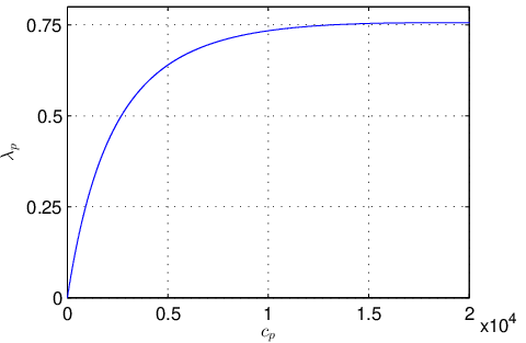
Numerical results with a varying rotational spring stiffness are now presented for the perfect system. The continuation and bifurcation software Auto-07p [2011] is used to solve the complete system of equilibrium equations presented in the previous section. An example set of section and material properties are chosen thus: , , , , , , , . The global critical load can be calculated using Equation (44), whereas the local buckling critical stress can be evaluated using the well-known formula , where the coefficient depends on the plate boundary conditions. By increasing the value, the relative rigidity between the main plate and the stiffener varies from being completely pinned () to fully-fixed (). Therefore the limiting values for are or for a long stiffener connected to the main plate with one edge free and the edge defining the junction between the stiffener and the main plate being taken to be pinned or fixed respectively [1970]. However, the value of the global critical buckling load remains the same since it is independent of .
To find the equilibrium path in the fundamental and post-buckling states, a similar solution strategy is performed as in recent work [2014, 2014], which is illustrated diagrammatically in Figure 5.


For a perfect strut, the initial post-buckling path is computed first from the critical buckling load with being varied. Many bifurcation points are detected on the weakly stable post-buckling path; the focus being on the one with the lowest value of , termed the secondary bifurcation point , see Figure 5(a). Note that the corresponding value is labelled as . For an imperfect strut, however, the equilibrium path is computed initially from zero axial load and then is increased up to the maximum value where a limit point is detected. The load subsequently drops and the path is asymptotic to the perfect path, as shown in Figure 5(b). If the joint stiffness is varied, the value of would be expected to increase, see Figure 5. This is owing to the local buckling critical stress increasing, which in turn causes the required global mode amplitude to trigger local buckling to increase also.
It is worth noting that for the perfect case, the model is in fact only valid where global buckling or stiffener local buckling is critical since the assumption is made such that the main plate can only buckle in sympathy with the stiffener. For the stiffener local buckling being critical, the bifurcation would occur when and a stable post-buckling path would initially emerge from the fundamental path. To include the main plate buckling locally first, the explicit link between and would have to be broken.
Figure 6


shows the numerical results from the example properties stated at the beginning of the current section. Initially, the results are presented for the perfect case where the joint between the main plate and the stiffener is pinned (). The graphs in (a–b) show the equilibrium plots of the normalized axial load versus the generalized coordinates of the sway component and the maximum out-of-plane normalized deflection of the buckled stiffener () respectively. The graph in (c) shows the relative amplitudes of global and local buckling modes in the post-buckling range. Finally, the graph in (d) shows the relationship between sway and tilt components of the global buckling mode, which are almost equal (difference approximately 0.05%); this indicates that the shear strain is small but, importantly, not zero. As found in Wadee and Farsi [2014], for the case where only the stiffener buckles locally, there is a sequence of snap-backs observed. This is the signature of cellular buckling [2000] and the cells are labelled . Figure 7

shows the corresponding progression of the numerical solutions for the local buckling functions and for cells , , and defined in Figure 6. It can be seen that the initially localized buckling mode progressively becomes more periodic as the system post-buckling advances.
By comparing the equilibrium paths against those for , it is observed that the snap-backs begin to vanish as is increased. Figure 8


shows the equilibrium paths for the strut with an increasingly rigid connection between the plate and the stiffener. In the graphs of the analytical results, the values of , in , are taken as 1, 100 and 500 respectively. The graphs in Figure 8(a–b) show the equilibrium path of the normalized axial load versus the normalized total end-shortening , see Equation (29), and the global mode amplitude respectively. It is found that increases with ; comparing for the highest value to the lowest value shown, it is seen to be nearly greater. Moreover, the post-buckling paths show a significantly stiffer response for higher values of . At , the maximum out-of-plane displacement for is approximately , whereas for , it is approximately . Figure 8(c) shows the normalized local versus global mode amplitudes and (d) shows the relationship of the ratio versus the rotational stiffness ; the final graph shows that the relationship flattens for larger values of , which would be expected as a fully rigid joint condition is approached.
4 Validation
The commercial FE software package Abaqus [2011] was first employed to validate the results from the analytical model. The same example set of section and material properties were chosen, as presented in §3. Four-noded shell elements with reduced integration (S4R) were used to model the structure. Rotational springs were also used along the length to simulate the rigidity of the main plate–stiffener joint. An eigenvalue analysis was used to calculate the critical buckling loads and eigenmodes. The nonlinear post-buckling analysis was performed with the static Riks method [1972] with the aforementioned eigenmodes being used to introduce the necessary geometric imperfection to facilitate this. In the current example, the rotational spring stiffness is assumed to be , which gives a value of and gives negligible rotation at the main plate–stiffener connection. Linear buckling analysis shows that global buckling is the first eigenmode; Table 1
| Source | Critical mode | |||
| Theory | Global | |||
| FE | Global | |||
| % difference | 0.12 | 3.09 | 7.31 | N/A |
presents the critical stresses for all the components from the analytical and the FE models.
Figure 9


shows the comparisons between the numerical results from the analytical and the FE models. It is shown for the case with an initial global imperfection and a local imperfection, where , , and for , which represents the initial imperfection for the analytical model that matches the FE model imperfection satisfactorily such that a meaningful comparison can be made. The graphs in (a–b) show the normalized axial load versus the global and the local mode amplitudes respectively; the graph in (c) shows the local versus the global buckling modal amplitudes. Figure 10

shows the local out-of-plane deflection profiles at the respective locations (i)–(iii), shown in Figure 9(a–c), the comparison being for the same value of . As can be seen, both sets of graphs show excellent correlation in all aspects of the mechanical response; in particular, the results for from the analytical and the FE model are almost indistinguishable. This shows a marked improvement on the previous simpler model [2014] where the main plate was assumed not to buckle locally. A visual comparison between the 3-dimensional representations of the strut from the analytical and the FE models is also presented in Figure 11.


4.1 Comparison with experimental study
An experimental study of a thin-walled stiffened plate conducted by Fok et al. [1976] also focused on the case where global buckling was critical. Two specific tests were conducted on a panel with multiple stiffeners. The experimental results were compared with the current analytical model and also with the FE model formulated in Abaqus. The cross-section of the stiffened panel investigated is shown in Figure 1. The experimental panel had blade stiffeners with spacing , height , thicknesses and (i.e. stiffeners on one side only). The experimental specimen was constructed from cold-setting Araldite® (epoxy resin) and the material had an elastic stress–strain relationship, but no material properties were provided. Hence, in the analytical and FE models, nominal values of and were used ( and as before); this did not pose a problem so long as the same values were used in both models. Moreover, it is worth noting that the behaviour of the experimental specimens was reported to be elastic and only ratios of loads and displacements were reported as the results [1976].
In the first test, the length of the panel was ensuring that the global critical buckling load was much less than the local buckling load. The initial global imperfection was measured to be but there were negligible out-of-plane imperfections in the stiffeners and in the main plate (i.e. were assumed). In the second test, the length of the stiffened panel was reduced to with the consequence that the local buckling stress was only approximately 5% above that for the global mode. The corresponding critical stresses for both tests are summarized in Table 2.
| Test 1 | ||||
|---|---|---|---|---|
| Test 2 |
For the panel, the initial global buckling mode imperfection was set to and the amplitude of the out-of-plane imperfection with , and . For both models, analytical and FE, the stiffness of the rotational spring was calibrated to be since this gave the best match with the peak load of the experimental results. To find the equilibrium path, the numerical continuation process was initiated from zero load. Figure 12


shows the comparisons between the experimental results from Fok et al. [1976], the analytical and the FE models. The comparisons show strong agreement between all three sets of results. Since there was no information provided about the local out-of-plane deflection magnitude, the results from the analytical model are compared to the FE results directly. Figure 13(a)


presents the comparison of the normalized force ratio versus the maximum normalized out-of-plane stiffener deflection , where the initial global and local imperfection sizes and shapes were given as before. Figure 13(b) shows the comparisons of the analytical with the FE model results for the local out-of-plane displacement of the stiffener for the Test 2 properties. Note that the results are obtained when (i) and (ii) . The comparison between the local buckling amplitudes and wavelength is excellent. Of course at lower loads, in the advanced post-buckling range, there is divergence between the non-midspan peaks; this is a further example of the FE model locking the modal wavelength as found in earlier studies even though actual experimental evidence shows the contrary [2008, 2012, 2014, 2014].
5 Concluding remarks
An analytical model based on variational principles has been extended to model local–global mode interaction in a stiffened plate subjected to uniaxial compression. By introducing the sympathetic deflection of the main plate along with the locally buckling stiffener, the current model could now be compared to published experiments [1976] and a finite element model formulated in Abaqus; results from both are found to be excellent. Currently, the authors are conducting an imperfection sensitivity study to quantify the parametric space for designers to avoid such dangerous structural behaviour, the results of which would provide greater understanding of the interactive buckling phenomena and highlight the practical implications.
References
- 2011 Abaqus. 2011. Version 6.10. Providence, USA: Dassault Systèmes.
- 2014 Bai, L., & Wadee, M. A. 2014. Mode interaction in thin-walled I-section struts with semi-rigid flange-web joints. Int. J. Non-Linear Mech. Submitted.
- 2008 Becque, J. 2008. The interaction of local and overall buckling of cold-formed stainless steel columns. Ph.D. thesis, School of Civil Engineering, University of Sydney, Sydney, Australia.
- 2009 Becque, J., & Rasmussen, K. J. R. 2009. Experimental investigation of the interaction of local and overall buckling of stainless steel I-columns. Asce journal of structural engineering, 135(11), 1340–1348.
- 1976 Budiansky, B. (ed). 1976. Buckling of structures. Berlin: Springer. IUTAM symposium.
- 1970 Bulson, P. S. 1970. The stability of flat plates. London, UK: Chatto & Windus.
- 2007 Burke, J., & Knobloch, E. 2007. Homoclinic snaking: Structure and stability. Chaos, 17(3), 037102.
- 2000 Butler, R., Lillico, M., Hunt, G. W., & McDonald, N. J. 2000. Experiment on interactive buckling in optimized stiffened panels. Structural and Multidisciplinary Optimization, 23(1), 40–48.
- 2009 Chapman, S. J., & Kozyreff, G. 2009. Exponential asymptotics of localised patterns and snaking bifurcation diagrams. Physica D, 238(3), 319–354.
- 2011 Doedel, E. J., & Oldeman, B. E. 2011. Auto-07p: Continuation and bifurcation software for ordinary differential equations. Montreal, Canada: Concordia University.
- 1976 Fok, W. C., Rhodes, J., & Walker, A. C. 1976. Local buckling of outstands in stiffened plates. Aeronautical Quarterly, 27, 277–291.
- 2006 Ghavami, K. G., & Khedmati, M. R. 2006. Numerical and experimental investigation on the compression behaviour of stiffened plates. J. Constr. Steel Res., 62(11), 1087–1100.
- 1999 Grondin, G. Y., Elwi, A. E., & Cheng, J. 1999. Buckling of stiffened steel plates – a parametric study. J. Constr. Steel Res., 50(2), 151–175.
- 1999 Guarracino, F., & Walker, A. 1999. Energy methods in structural mechanics. Thomas Telford.
- 1981 Hancock, G. J. 1981. Interaction buckling in I-section columns. ASCE J. Struct. Eng, 107(1), 165–179.
- 1998 Hunt, G. W., & Wadee, M. A. 1998. Localization and mode interaction in sandwich structures. Proc. R. Soc. A, 454(1972), 1197–1216.
- 1988 Hunt, G. W., Da Silva, L. S., & Manzocchi, G. M. E. 1988. Interactive buckling in sandwich structures. Proc. R. Soc. A, 417(1852), 155–177.
- 2000 Hunt, G. W., Peletier, M. A., Champneys, A. R., Woods, P. D., Wadee, M. A., Budd, C. J., & Lord, G. J. 2000. Cellular buckling in long structures. Nonlinear Dyn., 21(1), 3–29.
- 1976 Koiter, W. T., & Pignataro, M. 1976. A general theory for the interaction between local and overall buckling of stiffened panels. Tech. rept. WTHD 83. Delft University of Technology, Delft, The Netherlands.
- 2004 Loughlan, J. (ed). 2004. Thin-walled structures: Advances in research, design and manufacturing technology. Taylor & Francis.
- 1973 Murray, N. W. 1973. Buckling of stiffened panels loaded axially and in bending. The Structural Engineer, 51(8), 285–300.
- 2000 Pignataro, M., Pasca, M., & Franchin, P. 2000. Post-buckling analysis of corrugated panels in the presence of multiple interacting modes. Thin-Walled Struct., 36(1), 47–66.
- 1972 Riks, E. 1972. Application of Newton’s method to problem of elastic stability. Trans. ASME J. Appl. Mech, 39(4), 1060–1065.
- 1989 Ronalds, B. F. 1989. Torsional buckling and tripping strength of slender flat-bar stiffeners in steel plating. Proc. Instn. Civ. Engrs., 87(Dec.), 583–604.
- 2002 Schafer, B. W. 2002. Local, distortional, and Euler buckling of thin-walled columns. ASCE Journal of Structural Engineering, 128(3), 289–299.
- 2002 Sheikh, I. A., Grondin, G.Y., & Elwi, A. E. 2002. Stiffened steel plates under uniaxial compression. J. Constr. Steel Res., 58(5–8), 1061–1080.
- 1973 Thompson, J. M. T., & Hunt, G. W. 1973. A general theory of elastic stability. London: Wiley.
- 1984 Thompson, J. M. T., & Hunt, G. W. 1984. Elastic instability phenomena. London: Wiley.
- 2000 Wadee, M. A. 2000. Effects of periodic and localized imperfections on struts on nonlinear foundations and compression sandwich panels. Int. J. Solids Struct., 37(8), 1191–1209.
- 2014 Wadee, M. A., & Bai, L. 2014. Cellular buckling in I-section struts. Thin-Walled Struct., 81, 89–100.
- 2014 Wadee, M. A., & Farsi, M. 2014. Cellular buckling in stiffened plates. Proc. R. Soc. A, 470(2168), 20140094.
- 2012 Wadee, M. A., & Gardner, L. 2012. Cellular buckling from mode interaction in I-beams under uniform bending. Proc. R. Soc. A, 468(2137), 245–268.
- 1998 Wadee, M. A., & Hunt, G. W. 1998. Interactively induced localized buckling in sandwich structures with core orthotropy. Trans. ASME J. Appl. Mech., 65(2), 523–528.
- 2010 Wadee, M. A., Yiatros, S., & Theofanous, M. 2010. Comparative studies of localized buckling in sandwich struts with different core bending models. Int. J. Non-Linear Mech., 45(2), 111–120.
- 1997 Wadee, M. K., Hunt, G. W., & Whiting, A. I. M. 1997. Asymptotic and Rayleigh–Ritz routes to localized buckling solutions in an elastic instability problem. Proc. R. Soc. A, 453(1965), 2085–2107.
- 1999 Woods, P. D., & Champneys, A. R. 1999. Heteroclinic tangles and homoclinic snaking in the unfolding of a degenerate reversible Hamiltonian–Hopf bifurcation. Physica D, 129(3–4), 147–170.