Failure Inference and Optimization for Step Stress Model Based on Bivariate Wiener Model

S. Shemehsavar and Morteza Amini Note: ^* Corresponding author;
E-mail addresses: shemehsavar@khayam.ut.ac.ir (S. Shemehsavar), mortez.amini@ut.ac.ir (Morteza Amini). Affiliation: Department of Statistics, School of Mathematics, Statistics and Computer Sciences,College of Science, University of Tehran, P.O. Box 14155-6455, Tehran, Iran

Abstract

In this paper, we consider the situation under a life test, in which the failure time of the test units are not related deterministically to an observable stochastic time varying covariate. In such a case, the joint distribution of failure time and a marker value would be useful for modeling the step stress life test. The problem of accelerating such an experiment is considered as the main aim of this paper. We present a step stress accelerated model based on a bivariate Wiener process with one component as the latent (unobservable) degradation process, which determines the failure times and the other as a marker process, the degradation values of which are recorded at times of failure. Parametric inference based on the proposed model is discussed and the optimization procedure for obtaining the optimal time for changing the stress level is presented. The optimization criterion is to minimize the approximate variance of the maximum likelihood estimator of a percentile of the products’ lifetime distribution.

Keywords: Bivariate normal, Fisher information matrix, Inverse Gaussian distribution.
AMS subject classification: 62N05, 60K10

1 Introduction

The lifetime experiments have received attention recently, partly because the high reliability of the manufactured products is important in the current intense economical competition between trading firms. Over time, several lifetime tests for assessing the lifetime probability distribution of the products are developed, ranging from simple Constant Stress Life Test (CSLT) to the Step Stress Accelerated Degradation Test (SSADT). Two useful survey of available results are given in the books of Nelson ,1990 and Bagdonavicius and Nikulin, 2010. For some recent papers concerning the lifetime experiments see Pan and Balakrishnan, 2010, Pan et al., 2011, Jin, 2011, Simino et al., 2012 and Wang et al., 2012.

Life tests usually deal with models for which failure occurs when an observable degradation process crosses a threshold level. However, there are practical situations in which the failure time of the test units are not related deterministically to an observable marker covariate. In such a case, the joint distribution of the failure time and a marker process would be useful for modeling the step stress life test. Joint models for marker evolution and failure are proposed in the literature under the simple constant stress life tests, including Jewell and Kalbfleisch, 1996, who examine jump processes for markers and an additive relationship between the marker and the failure time hazard function, and Yashin and Manton, 1997, who consider diffusion processes for markers along with a quadratic relationship between the hazard function and markers.

In most cases, the information about the latent (unobservable) degradation path can only be obtained using the related marker(s) and the fact that a failure occurs when the latent degradation process crosses a known threshold. Whitmore et al., 1998, proposed a constant stress bivariate Wiener model in which one component represents the marker and the second, which is latent, determines the failure time.

The constant stress life tests are usually very costly, since they require destroying a considerable number of products for testing at each level of stress. To handle this problem, Step Stress Accelerated Life Tests (SSALT) were proposed as an economic alternative to the constant stress life tests. In a SSALT framework, each product is first tested, subject to a pre-determined stress level for a specified duration, and the failure data are collected. A product which survived until the end of the first step was again tested at a higher stress level and for a different time duration. The experiment is repeated for a specified number of stress levels and terminated at a pre-determined censoring time. The constant stress bivariate Wiener model proposed by Whitmore et al., 1998 is as well a costly experiment. Although censoring in this model decreases the total time of the experiment it does not solve the problem of efficiency. To handle this problem, we consider a SSALT design under the bivariate Wiener model.

An essential problem in an SSALT design is to determine the optimal time for changing the stress level by the experimenter. The problem of optimizing the test design have been extensively studied in recent years. Three commonly used optimization criteria are the minimum Approximated variance (Avar) of the Maximum Likelihood Estimators (MLE) of reliability, Mean Time To Failure (MTTF) and the quantiles of the population. For surveys of recent results in optimization of life test designs, see in particular Tang et al., 2004, Liao and Tseng, 2006 and Tseng et al., 2009.

In this paper, we reconstruct the model proposed by Whitmore et al., 1998 in a SSALT framework. Such a generalized model is clearly more economic than the constant stress model of Whitmore et al., 1998, since constant stress experiment requires destroying a considerable number of products at each level of stress. The Maximum likelihood and Bayesian estimation of the parameters of the proposed model are discussed. Next, we determine the optimal stress changing time by minimizing the Avar of the MLE of the 100 $p^{\mbox{th}}$ percentile of the products’ life time distribution.

The rest of this paper is organized as follows. In Section 2, we introduce the SSALT model with a bivariate Wiener process and derive the joint distribution of failure times and the marker process. Parametric Inference based on the proposed model is discussed in Section 3. The optimization criterion is described in Section 4. Finally an illustrative example is presented in Section 5.

2 The Model

Consider a two-dimensional Wiener diffusion process $\{(X(r),Y(r))\}$ , for $r\geq 0$ with $(X(0),Y(0))=(0,0)$ (see Cox and Miller, 1965). In other words, under the normal stress level $S_{0}$

(X(r),Y(r))|S_{0}\sim N_{2}(r{\mu_{X}}_{0},r{\mu_{Y}}_{0},r\sigma^{2}_{X},r\sigma^{2}_{Y},\rho),

where $N_{2}$ stands for the bivariate normal distribution. Assume further that ${\mu_{X}}_{0}\geq 0$ , which guarantees the degradation process $X(r)$ to be stochastically increasing in $r$ .

The component $X(r)$ assumed to be a degradation process that represents the level of deterioration of an item. An item fails as soon as $X(r)$ reaches a threshold $D>0$ . This first passage time of the degradation process through the threshold is denoted by a random variable $T$ , namely

T=\inf\{t|X{(t)}\geq D\}.

(2.1)

The failure time $T$ follows an inverse Gaussian distribution (see for instance, Chhikara and Folks, 1989), with the cumulative distribution function (cdf) under the normal stress level $S_{0}$ as follows

G_{0}(t)=\Phi\left(\sqrt{\frac{1}{\sigma_{X}^{2}t}}({\mu_{X}}_{0}t-D)\right)+exp\left\{\frac{2{\mu_{X}}_{0}D}{\sigma_{X}^{2}}\right\}\Phi\left(-\sqrt{\frac{1}{\sigma_{X}^{2}t}}({\mu_{X}}_{0}t+D)\right),

(2.2)

where $\Phi$ is the cdf of the standard normal distribution.

The degradation process $X(r)$ is assumed to be unobservable. The component $Y(r)$ represents a marker process that is correlated with the degradation process and tracks its progress. Thus, results of the experiment are based on observations on the marker process, supplemented by failure times of failed items. We focus on the situation where marker measurements are taken only at the failure or censoring times.

Consider the above bivariate process to model a SSALT problem. Under a SSALT, each item is first tested subject to a stress level $S_{1}$ ( $S_{1}>S_{0}$ ) for a specified duration $[0,\tau_{1})$ . If the item does not fail, it is tested again at a higher stress level $S_{2}$ ( $S_{2}>S_{1}$ ) for another specified duration $[\tau_{1},\tau_{2})$ . The experiment is continued until the time $C$ , under $m\geq 2$ stress levels $S_{m}>S_{m-1}>\cdots>S_{2}>S_{1}$ . The stress level of the experiment is then defined as

S=\left\{\begin{array}[]{l l}S_{1}&\mbox{for}\;\;0\leq t<\tau_{1}\\ S_{2}&\mbox{for}\;\;\tau_{1}\leq t<\tau_{2}\\ \vdots&\\ S_{m}&\mbox{for}\;\;\tau_{m-1}\leq t<C,\end{array}\right.

where the pre-specified values $0<\tau_{1}<\tau_{2}<\cdots<\tau_{m-1}<C$ are called the stress changing times.

Refer to caption — Figure 1: A sampler degradation path. Three different paths are showed: a failed item under the first stress level (dashed line), a failed item under the second stress level (dotted line) and a survived (censored) item (dash-dotted line).

Under a SSALT model, each item has two possible observation outcomes during the period $(0,C]$ :

•

Surviving (Censored) item: The item survives to the censoring time $C$ at which a marker level of $Y(C)=y(C)$ is recorded. This occurrence constitutes a censored observation of failure time with $T>C$ .
•

Failing item: The items fails at some time $T=t$ during the period $(0,C]$ and a marker level of $Y(T)=y(t)$ is recorded at the moment of failure.

2.1 The distribution of failure time and marker covariate

For the aforementioned plan, under the stress $S_{j},$ for $j=1,2,\ldots,m$ , we have

(X(r),Y(r))|S_{j}\sim N_{2}(r\mu_{X_{j}},r\mu_{Y_{j}},r\sigma^{2}_{X},r\sigma^{2}_{Y},\rho).

Assume further that the Arrhenius reaction model is used to model the relationship between the location parameters $\mu_{X_{j}}$ and $\mu_{Y_{j}}$ and the temperature stress $S_{j}$ , that is

\mu_{X_{j}}=\exp\left(a+\frac{b}{273+S_{j}}\right),\;\mu_{Y_{j}}=\exp\left(c+\frac{d}{273+S_{j}}\right),\;j=0,1,\ldots,m.

(2.3)

Consider any sample path of the component $X$ , under stress $S_{j}$ , over a time interval $(0,r]$ and partition this sample path at arbitrary time points $0=r_{0}<r_{1}\cdots<r_{k}=r,\;k\geq 1$ . Let $\Delta r_{i}=r_{i}-r_{i-1}$ and $\Delta x_{i}=x(r_{i})-x(r_{i-1})$ , for $i=1,\cdots,k$ . Denote the set of realized increments $\{\Delta x_{1},\ldots,\Delta x_{k}\}$ by $P$ . Then we have clearly

Y{(r)}|P\sim N(\mu_{y.x(r)},r\sigma^{2}_{Y}(1-\rho^{2})),

(2.4)

where for $j=1,\ldots,m,$

\mu_{y.x(r)}=\mu_{j}(y,r)+\rho\frac{\sigma_{Y}}{\sigma_{X}}[x(r)-\mu_{j}(x,t)],\quad\tau_{j-1}\leq r<\tau_{j},

\mu_{j}(y,t)=\mu_{Y_{j}}(t-\tau_{j-1})+\sum_{k=1}^{j-1}\mu_{Y_{k}}(\tau_{k}-\tau_{k-1}),

\mu_{j}(x,t)=\mu_{X_{j}}(t-\tau_{j-1})+\sum_{k=1}^{j-1}\mu_{X_{k}}(\tau_{k}-\tau_{k-1}),

$\tau_{0}=0$ and $\tau_{m}=C$ .

The conditional distribution in (2.4) is the same as the conditional distribution $Y{(r)}|x(r)$ . Hence (2.4) holds for any sample path of $X$ .

Therefore, for a surviving path, the conditional distribution of the marker given the degradation at the censoring time $C$ is as follows

Y{(C)}|X(C)\sim N(\mu_{y.x(C)},C\sigma^{2}_{Y}(1-\rho^{2})).

The resulting conditional probability density function (p.d.f) of the surviving path then is

p_{1}(y|x;\theta)=C^{-1/2}\sigma^{-1}_{Y}(1-\rho^{2})^{-1/2}\phi\left(C^{-1/2}\sigma^{-1}_{Y}(1-\rho^{2})^{-1/2}(y-\mu_{y.x(C)})\right),

(2.5)

where $\phi$ is the pdf of the standard normal distribution and

\theta=(\mu_{X1},\ldots,\mu_{Xm},\mu_{Y1},\ldots,\mu_{Ym},\sigma_{X}^{2},\sigma_{Y}^{2},\rho).

For a failing item at time $t$ , the distribution of $Y{(t)}|x(t)$ is equal to (2.4) with $r$ replaced by $t$ and $x(r)$ replaced by $x(t)=D$ . The corresponding p.d.f then is

p_{2}(y|t;\theta)=t^{-1/2}\sigma^{-1}_{Y}(1-\rho^{2})^{-1/2}\phi\left(t^{-1/2}\sigma^{-1}_{Y}(1-\rho^{2})^{-1/2}\left(y-\mu_{j}(y,t)+\rho\frac{\sigma_{Y}}{\sigma_{X}}[D-\mu_{j}(x,t)]\right)\right).

A similar argument to that in Lu, 1995 can be used to derive the p.d.f. of a surviving item, that is ${\rm P}(X(C)=x,T>C)$ , as follows

p_{3}(x)=\frac{1-exp(-\frac{2D(D-x)}{\sigma^{2}_{X}C})}{\sigma_{X}\sqrt{C}}\phi(\frac{x-\mu_{m}(x,C)}{\sigma_{X}\sqrt{C}}),\quad-\infty<x<D.

(2.6)

It is easy to verify that the p.d.f. of $T$ in (2.1) of a failing item is

f_{T}(t|T<C)=\sum_{j=1}^{m}\frac{D}{\sqrt{(2\pi\sigma^{2}_{X}t^{3})}}exp(-\frac{(D-\mu_{X_{j}}t)^{2}}{2\sigma^{2}_{X}t})I_{(\tau_{j-1},\tau_{j})}(t),

where

I_{A}(t)=\left\{\begin{array}[]{lr}1\;\;\mbox{if}&t\in A\\ 0\;\;\mbox{if}&t\notin A,\end{array}\right.

$\tau_{0}=0$ and $\tau_{m}=C$ .

We combine the preceding results to obtain the p.d.f. for each type of observation outcome, as follows:

For a censored item which survives beyond time $C$ , the joint p.d.f. of the marker $Y(C)$ and the latent degradation $X(C)$ is given by $p_{1}(y|x;\theta)p_{3}(x;\theta)$ , where $p_{1}$ and $p_{3}$ are given in (2.5) and (2.6), respectively. Since the $X(C)=x$ is not observed, we integrate it out of the joint density to obtain

P_{C_{m}}(y;\theta)=P(Y(C)=y,T>C)=\int_{-\infty}^{D}p_{1}(y|x;\theta)p_{3}(x;\theta)dx.

(2.7)

For a failing item, the joint p.d.f of $Y(T)$ and $T$ equals

P_{f}(y,t;\theta)=P(Y(T)=y,T=t<C)=p_{2}(y|t;\theta)f_{T}(t;\theta).

(2.8)

2.2 The likelihood

Assume that $n$ items are on test subject to SSADT over the observation period $(0,C]$ . The sample log-likelihood then is given by

	$\displaystyle\log L(\theta)$	$\displaystyle=$	$\displaystyle\sum_{i=1}^{n}\sum_{j=1}^{m}I_{(\tau_{j-1},\tau_{j})}(t_{i})\log P_{f}(y_{i},t_{i};\theta)+(1-I_{(0,C)}(t_{i}))\log P_{C_{m}}(y_{i};\theta)$		(2.9)
		$\displaystyle=$	$\displaystyle\sum_{j=1}^{m}\sum_{i=\xi_{j-1}+1}^{\xi_{j}}\log P_{f_{j}}(y_{i},t_{i};\theta)+\sum_{i=\xi_{m-1}+1}^{n}\log P_{C_{m}}(y_{i};\theta).$		(2.9)

$\xi_{j}=\sum_{k=0}^{j}\nu_{k}$ and $\nu_{0}=0$ , in which $\nu_{j}$ is the number of failed items under stress $S_{j}$ , for $j=1,\ldots,m$ , $(y_{k},t_{k})$ , for $k=\xi_{j-1}+1,\ldots,\xi_{j}$ , denote the sample failing items for the stress level $S_{j},\;j=1,\ldots,m$ , $y_{k}$ , for $k=\xi_{m-1}+1,\ldots,n,$ denote the sample surviving (censored) items,

P_{fj}(y_{i},t_{i};\theta)=I_{(\tau_{j-1},\tau_{j})}(t_{i})\;D(2\pi\sigma_{X}\sigma_{Y})^{-1}(1-\rho^{2})^{-1/2}t_{i}^{-2}e^{-t_{i}^{-1}Q_{j(y_{i},t_{i})}},\quad j=1,\ldots,m,

Q_{j}(y,t)=\eta_{1}(q_{j}(t,y)-\eta_{2}P_{j}(t))^{2}+\sigma_{X}^{-2}(D-\mu_{Xj}t)^{2}/2,,\quad j=1,\ldots,m,

q_{j}(t,y)=y-\mu_{j}(y,t),\quad P_{j}(t)=D-\mu_{j}(x,t),\quad j=1,\ldots,m,

in which

\eta_{1}=\sigma_{Y}^{-2}(1-\rho^{2})^{-1}/2,\quad\mbox{and}\quad\eta_{2}=\rho\sigma_{Y}\sigma_{X}^{-1}.

(2.10)

Furthermore, integrating (2.7) results in

P_{C_{m}}(y_{i};\theta)=c_{y}\sum_{k=1}^{2}(-1)^{k-1}e^{(k-1)\beta_{m}}\Phi(c_{m}(y;k,1))\phi(c_{m}(y;k,2)),

where

c_{y}=\sigma_{Y}^{-1}C^{-1/2},\quad\beta_{m}=2D(D-P_{m}(C))\sigma_{X}^{-2}C^{-1},

c_{m}(y;1,1)=\eta_{3}(P_{m}(C)-\rho\sigma_{X}\sigma_{Y}^{-1}q_{m}(C,y)),\quad c_{m}(y;1,2)=c_{y}q_{m}(C,y),

c_{m}(y;2,1)=\eta_{3}(P_{m}(C)-\rho\sigma_{X}\sigma_{Y}^{-1}q_{m}(C,y)-2D(1-\rho^{2})),\quad c_{m}(y;2,2)=c_{y}(q_{m}(C,y)-2\eta_{2}D),

and

\eta_{3}=\sigma_{X}^{-1}(1-\rho^{2})^{-1/2}C^{-1/2}.

(2.11)

3 Parametric Inference

In this section, we develop the parametric inferential procedures based on the proposed models. The maximum likelihood and Bayesian estimation methods are considered for inferential purpose. From Section 2, it is apparent that the models are analytically intractable. Thus, the finite sample performance of the maximum likelihood and Bayesian estimators could be examined through a simulation study. To perform a simulation study, we set $m=2$ , $D=1$ , $C=700$ , $S_{1}=1200$ , $S_{2}=1400$ , and $\tau=300,400,500$ . Because of the invariance property of the maximum likelihood estimators, the maximum likelihood estimates of the parameter vector $\theta=(\mu_{X_{1}},\mu_{X_{2}},\mu_{Y_{1}},\mu_{Y_{2}},\sigma^{2}_{X},\sigma^{2}_{Y},\rho)$ and those of the transformed parameter vector

\theta^{*}=(a,b,c,d,\sigma^{2}_{X},\sigma^{2}_{Y},\rho)

can be obtained from each other. In the following, we assume the transformed parameter vector $\theta^{*}$ as in Table 1.

Table 1: Parameter of model used for the simulation

$\theta^{*}$	a	b	c	d	$\sigma^{2}_{X}$	$\sigma^{2}_{Y}$	$\rho$
	-2.817991	-4996.008	-1.644788	-4995.996	0.001729986	0.0020806801	0.5893698756

Using (2.3) we have $(\mu_{X_{1}},\mu_{X_{2}},\mu_{Y_{1}},\mu_{Y_{2}})=(0.002009813,0.00301472,0.006496424,0.009744636)$ .

3.1 Maximum likelihood

First, we deal with maximum likelihood estimation of the model parameters. Suppose $n=30$ independent items are tested subject to SSALT over the observation period $(0,C]$ . The maximum likelihood estimators (MLEs) of the model parameters can be obtained by maximizing the log-likelihood (2.9). It is not possible to obtain the MLEs of the parameters in a closed form. Thus, numerical computational methods are used for obtaining the MLEs. A Monté Carlo simulation with 10,000 iterations is conducted using software R 2.14.2 to obtain the estimated relative root of mean square error (RRMSE) and estimated relative bias (Rbias) of the ML estimators of the parameters. These results are summarized in Table 2. One can observe from Table 2 that the performance of the estimates are quite satisfactory in terms of RRMSE and Rbias.

Table 2: Parameter estimates for

\tau=300,\;400,\;500,\;n=30

$\tau$		$\mu_{X_{1}}$	$\mu_{X_{2}}$	$\mu_{Y_{1}}$	$\mu_{Y_{2}}$	$\sigma^{2}_{X}$	$\sigma^{2}_{Y}$	$\rho$
	MLE	0.001544	0.002315	0.006268	0.009401	0.001755	0.002020	0.591156
300	Rbias	-0.231723	-0.154533	-0.035092	-0.035226	0.014603	-0.029246	0.003031
	RRMSE	0.263621	0.175785	0.063134	0.063224	0.271781	0.245912	0.204330
	MLE	0.001536	0.002303	0.006277	0.009415	0.001839	0.002045	0.596587
400	Rbias	-0.236005	-0.157394	-0.033721	-0.033851	0.062744	-0.017047	0.012246
	RRMSE	0.275125	0.183462	0.063961	0.064030	0.271558	0.248880	0.203052
	MLE	0.001599	0.002396	0.006324	0.009484	0.001850	0.002050	0.596866
500	Rbias	-0.204660	-0.13650	-0.026547	-0.026784	0.069158	-0.014685	0.012720
	RRMSE	0.262404	0.174980	0.063265	0.064235	0.273821	0.246177	0.204354

Table 3: Thirty simulated observation for parameter set of Table 1.

	$\tau=300$			$\tau=400$			$\tau=500$
$\delta$	t	y	$\delta$	t	y	$\delta$	t	y
1	206	2.9043836	1	125	1.3302026	1	72	0.8630739
1	204	2.2834415	1	347	2.0791452	3	700	5.7413420
2	358	2.0369846	2	409	2.8987105	1	257	0.5140461
2	424	2.2286551	3	700	4.3707818	2	627	3.7818455
2	528	3.3882536	1	321	4.2948213	1	265	2.5664485
1	293	1.0765821	2	664	5.1428573	3	700	2.3397970
2	433	3.4253562	2	413	2.1084361	2	588	4.4356021
2	367	2.7105020	2	575	3.8347019	1	261	2.2925127
2	481	2.7411018	3	700	4.3353895	1	152	1.5052757
1	74	0.4584009	1	61	1.4195226	1	203	2.2968604
1	232	1.4229018	2	443	4.7402742	3	700	5.2271200
2	563	2.0737839	1	74	0.9594538	1	205	2.4270830
2	524	4.6559941	3	700	6.6440064	2	500	3.9215091
2	398	3.0469754	2	439	2.2434726	3	700	4.2650212
1	83	1.1645206	2	543	3.6592403	2	521	2.0058003
1	288	1.5370298	3	700	3.9542721	1	321	3.1932579
2	518	2.8000903	1	238	0.4759539	1	435	3.1052309
2	558	4.4736314	1	104	1.2579545	1	160	2.6871790
1	106	1.3271670	2	413	2.6969144	1	329	3.0110215
1	699	7.4817986	2	429	1.5348759	2	687	5.7361510
2	538	4.5781005	1	231	0.9987282	1	249	1.9830004
1	98	0.3647197	1	205	2.1099217	2	578	2.8660246
1	184	1.5738009	3	700	6.1866970	1	335	2.4279700
2	379	2.8413248	1	146	1.8776734	1	273	2.3275245
1	102	1.1580797	3	700	4.6567010	1	143	1.3927807
1	165	1.6696197	1	375	1.5709192	1	161	2.3288032
2	584	3.6045384	2	541	2.8358232	2	692	5.5437838
2	371	2.4435304	2	600	4.1900476	1	175	0.7888585
2	538	4.4705936	2	623	3.8115301	1	199	1.0319427
2	303	2.8150623	1	274	2.0937201	3	700	3.1902784

3.2 Bayesian approach

The Bayesian approach is appealing to statisticians and reliability engineers, since it provides a method of using their past experiences and/or prior convictions for inference. From a Bayesian point of view, we can treat the unknown parameters as a random variable with a known prior probability distribution. Then, we can combine information from the random sample and prior probability distribution to obtain the Bayesian estimators for the parameters of the model. However, in most practical applications, where the Bayesian approach is used, it is difficult to compute analytically the posterior distribution. The Markov chain Monté Carlo (MCMC) method uses to generate a sample from the posterior distribution large enough so that any desired feature of the posterior distribution can be accurately obtained. Because of the restrictions $\mu_{X_{1}}<\mu_{X_{2}}$ and $\mu_{Y_{1}}<\mu_{Y_{2}}$ , we have to consider joint priors for the vectors $(\mu_{X_{1}},\mu_{X_{2}})$ and $(\mu_{Y_{1}},\mu_{Y_{2}})$ , while we can consider independent priors for the transformed parameters $a,b,c$ and $d$ . To simplify the calculations, we perform the Bayesian approach for the transformed parameter vector $\theta^{*}=(a,b,c,d,\sigma^{2}_{X},\sigma^{2}_{Y},\rho)$ .

Table 4: Parameter estimation results for

\tau=300,\;400,\;500,\;n=30

			$\tau=300$
	Mean	Std	MC-er	2.5 $\%$	Medain	97.5 $\%$
a	-3.21803700	0.1809108	0.0009045538	-3.562406	-3.185069	-2.991624
b	-4100.17100	317.9782	1.589891	-4624.464	-4109.659	-3580.026
c	-2.24168800	0.2151238	0.001075619	-2.586862	-2.256567	-1.897493
d	-4085.98400	353.0725	1.765363	-4670.439	-4076.054	-3539.374
$\sigma^{2}_{X}$	0.001651598	0.00001052115	5.260574 $\times 10^{-8}$	0.001635779	0.001649452	0.001679365
$\sigma^{2}_{Y}$	0.002155083	0.00007563872	3.781936 $\times 10^{-7}$	0.00203197	0.002152928	0.002293804
$\rho$	0.594830600	0.03566883	1.783442 $\times 10^{-4}$	0.5374839	0.5871186	0.6582097
			$\tau=400$
	Mean	Std	MC-er	2.5 $\%$	Medain	97.5 $\%$
a	-3.318978	0.1811505	0.0009057527	-3.599276	-3.355476	-3.028328
b	-4070.080	300.5802	1.502901	-4603.892	-4046.055	-3633.086
c	-2.245963	0.1760872	0.0008804360	-2.539122	-2.250249	-1.975724
d	-4102.815	301.8582	1.509291	-4586.286	-4105.338	-3627.138
$\sigma^{2}_{X}$	0.001817105	5.632395 $\times 10^{-5}$	2.816198 $\times 10^{-7}$	0.001746018	0.001798002	0.001932355
$\sigma^{2}_{Y}$	0.001924476	3.424275 $\times 10^{-5}$	1.712138 $\times 10^{-7}$	0.001872394	0.001920889	0.001980292
$\rho$	0.5896328	0.01278770	6.393848 $\times 10^{-5}$	0.5574416	0.5901468	0.6118633
			$\tau=500$
	Mean	Std	MC-er	2.5 $\%$	Medain	97.5 $\%$
a	-3.204618	0.1443177	0.0007215886	-3.447255	-3.158764	-2.968463
b	-4151.146	312.5983	1.562992	-4692.574	-4130.741	-3667.357
c	-2.250095	0.1716518	0.0008582590	-2.545561	-2.212597	-1.971093
d	-4090.401	288.7204	1.443602	-4581.323	-4123.713	-3607.695
$\sigma^{2}_{X}$	0.001729962	0.00005117870	2.558935 $\times 10^{-7}$	0.001638141	0.001740245	0.001804733
$\sigma^{2}_{Y}$	0.002047766	0.00003888018	1.944009 $\times 10^{-7}$	0.001976453	0.002049934	0.002135915
$\rho$	0.5792594	0.01128655	5.643275 $\times 10^{-5}$	0.5586604	0.5785074	0.6028768

Table 5: Parameter estimates for non informative prior

\tau=300,\;400,\;500,\;n=30

					$n=30$
$\tau$		$\mu_{X_{1}}$	$\mu_{X_{2}}$	$\mu_{Y_{1}}$	$\mu_{Y_{2}}$	$\sigma^{2}_{X}$	$\sigma^{2}_{Y}$	$\rho$
	BE	0.002479	0.003456	0.006636	0.009242	0.001652	0.002155	0.594831
300	Rbias	0.233561	0.146273	0.021469	-0.05154	-0.045311	0.035759	0.009265
	MC-er	7.27 $\times 10^{-7}$	8.05 $\times 10^{-7}$	8.73 $\times 10^{-7}$	1.31 $\times 10^{-5}$	1.05 $\times 10^{-5}$	7.56 $\times 10^{-5}$	0.000178
	BE	0.002285	0.003178	0.006534	0.009112	0.001817	0.001924	0.589633
400	Rbias	0.136740	0.054138	0.005756	-0.064964	0.050358	-0.075074	0.000446
	MC-er	3.80 $\times 10^{-7}$	3.61 $\times 10^{-7}$	1.08 $\times 10^{-6}$	1.29 $\times 10^{-5}$	2.82 $\times 10^{-7}$	1.71 $\times 10^{-6}$	6.39 $\times 10^{-5}$
	BE	0.002430	0.003399	0.006568	0.009141	0.001730	0.002048	0.579259
500	Rbias	0.209242	0.127457	0.009893	-0.006195	-0.000014	-0.015819	-0.017155
	MC-er	9.35 $\times 10^{-7}$	9.50 $\times 10^{-7}$	8.70 $\times 10^{-7}$	1.29 $\times 10^{-5}$	2.56 $\times 10^{-7}$	1.94 $\times 10^{-7}$	5.64 $\times 10^{-5}$

Table 3 presents simulated data sets by using the parameters in Table 1 for $\tau=300,400,500$ . We consider the Bayes estimation of the transformed parameter vector, ${\theta}^{*}$ , based on data sets in Table 3, under the square error and absolute error loss functions. An analytic calculation of estimators and their risks for comparison is far from reach. To carry out an empirical comparison, a simulation study was conducted using software R 2.14.2 to generate a sequence of parameter values from the posterior density of $\theta^{*}$ given the generated data set of Table 3 by making use of the random walk Metropolis-Hasting algorithm.

To facilitate the Bayesian approach, we assume independent prior distributions for the model parameters, that is

\pi(a,b,c,d,\sigma^{2}_{X},\sigma^{2}_{Y},\rho)\propto\pi_{1}(a)\pi_{2}(b)\pi_{3}(c)\pi_{4}(d)\pi_{5}(\sigma^{2}_{X})\pi_{6}(\sigma^{2}_{Y})\pi_{7}(\rho),

where $\pi_{1}(a),\;\pi_{2}(b),\;\pi_{3}(c)$ and $\pi_{4}(d)$ are assumed to be the low informative normal densities with zero mean and the variance equal to $10^{4}$ , $\pi_{5}(\sigma^{2}_{X})$ and $\pi_{6}(\sigma^{2}_{Y})$ are assumed to be the non-informative Jeffrey’s priors $\pi(\sigma^{2}_{X})\propto\frac{1}{\sigma^{2}_{X}},\;\pi(\sigma^{2}_{Y})\propto\frac{1}{\sigma^{2}_{Y}}$ and $\pi_{7}(\rho)$ is taken to be the non-informative uniform $(-1,1)$ prior.

The random walk Metropolis-Hasting algorithm is executed 50000 times and the last 40000 were used for the sake of convergency. The empirical posterior densities of the model parameters and two dimensional plots of the generated model parameters $(a,b,c,d)$ are shown in Figures 2 and 3, respectively, for $\tau=400$ . Using these empirical densities we estimate the mean, standard deviation (Std), MCMC error (MC-er), the median and other critical quantiles of parameters. These numerical results are summarized in Table 4.

For the sake of brevity, only the values of the Bayse estimates (BEs) based on the square error loss, as well as their Rbias, MC-er were typically given in Table 5 to be compared with the corresponding values of the ordinary MLEs. Similar comparisons can be made between BEs based on the absolute error loss and the MLEs.

4 Optimal test plan

For $m=2$ stress levels, we have

\mu_{X0}=\exp\left(\frac{\log\mu_{X1}-\alpha\log\mu_{X2}}{1-\alpha}\right)\\ \mbox{and}\\ \mu_{Y0}=\exp\left(\frac{\log\mu_{Y1}-\alpha\log\mu_{Y2}}{1-\alpha}\right),\\

(4.1)

where

\alpha=\frac{S_{1}-S_{0}(273+S_{2})}{S_{2}-S_{0}(273+S_{1})}

is called the stress ratio.

The optimization criterion considered in this paper has to find the optimal stress changing time $0<\tau^{*}<C$ which minimizes the Approximate variance (Avar) of the ML estimate of the 100 $p^{\mbox{th}}$ percentile of the distribution of $T$ , $\hat{\xi}_{p}$ , under the normal stress level $S_{0}$ . The Avar of $\hat{\xi}_{p}$ is a function of the stress changing time $\tau$ and the parameter vector $\theta$ . Hence, before performing the optimization procedure, one have to estimate the parameter vector $\theta$ using a lifetime data in normal conditions. This is done via the ML estimation using (2.9) and based on a pilot study.

The Avar of $\hat{\xi}_{p}$ can be obtained as a function of the approximated variance of the MLE of $\theta$ ( the inverse of the Fisher information matrix, $I(\theta)$ ), using the delta method as

\mbox{Avar}(\hat{\xi}_{p})=H^{\prime}I^{-1}(\theta)H/(f_{T_{0}}(\hat{\xi}_{p}))^{2},

where $f_{T_{0}}(t)$ is the corresponding pdf of $G_{0}(t)$ in (2.2) and

H^{\prime}=\left[\frac{\partial\hat{{G}}_{0}(\hat{\xi}_{p})}{\partial\hat{\mu}_{X1}},\frac{\partial\hat{{G}}_{0}(\hat{\xi}_{p})}{\partial\hat{\mu}_{X2}},0,0,\frac{\partial\hat{{G}}_{0}(\hat{\xi}_{p})}{\partial\hat{\sigma}_{X}^{2}},0,0\right].

Note that ${{G}}_{0}(s)$ is not a function of ${\mu}_{Y1},{\mu}_{Y2},{\sigma}_{Y}^{2}$ , and $\rho$ .

We have

\displaystyle\frac{\partial\hat{{G}}_{0}(\hat{\xi}_{p})}{\partial\hat{\mu}_{X_{1}}}

\displaystyle=

\displaystyle\frac{\hat{\xi}_{p}\hat{\mu}_{X_{0}}\phi\left(c_{1x}\right)}{\hat{\mu}_{X_{1}}(1-\alpha)\sqrt{\hat{\sigma}_{X}^{2}\hat{\xi}_{p}}}+\frac{2D\hat{\mu}_{X_{0}}e^{\beta_{3}}}{\hat{\mu}_{X_{1}}\hat{\sigma}_{X}^{2}(1-\alpha)}\Phi\left\{c_{2x}\right\}-\frac{\hat{\xi}_{p}\hat{\mu}_{X_{0}}e^{\beta_{3}}}{\hat{\mu}_{X_{1}}(1-\alpha)\sqrt{\hat{\sigma}_{X}^{2}\hat{\xi}_{p}}}\phi\left\{c_{2x}\right\},

\frac{\partial\hat{{G}}_{0}(\hat{\xi}_{p})}{\partial\hat{\mu}_{X_{2}}}=-\alpha\frac{\hat{\mu}_{X_{1}}}{\hat{\mu}_{X_{2}}}\frac{\partial\hat{{G}}_{0}(\hat{\xi}_{p})}{\partial\hat{\mu}_{X_{1}}},

and

\displaystyle\frac{\partial\hat{{G}}_{0}(\hat{\xi}_{p})}{\partial\hat{\sigma}_{X}^{2}}

\displaystyle=

\displaystyle-\frac{\left[\hat{\mu}_{X_{0}}\hat{\xi}_{p}-D\right]\phi\left(c_{1x}\right)}{2\hat{\sigma}_{X}^{3}\sqrt{\hat{\xi}_{p}}}-\frac{2D\hat{\mu}_{X_{0}}e^{\beta_{3}}\Phi\left\{c_{2x}\right\}}{\hat{\sigma}_{X}^{4}}+\frac{\left[\hat{\mu}_{X_{0}}\hat{\xi}_{p}+D\right]e^{\beta_{3}}\phi\left\{c_{2x}\right\}}{2\hat{\sigma}_{X}^{3}\sqrt{\hat{\xi}_{p}}}.

where

c_{1x}=\sqrt{\frac{1}{\hat{\sigma}_{X}^{2}\hat{\xi}_{p}}}\left[\hat{\mu}_{X_{0}}\hat{\xi}_{p}-D\right],\quad c_{2x}=-\sqrt{\frac{1}{\hat{\sigma}_{X}^{2}\hat{\xi}_{p}}}\left[\hat{\mu}_{X_{0}}\hat{\xi}_{p}+D\right],

\beta_{3}=\frac{2D}{\hat{\sigma}_{X}^{2}}\hat{\mu}_{X_{0}},\quad\hat{\mu}_{X_{0}}=\exp\left(\frac{\log\hat{\mu}_{X_{1}}-\alpha\log\hat{\mu}_{X_{2}}}{1-\alpha}\right)

and $\hat{\mu}_{X1}$ , $\hat{\mu}_{X2}$ and $\hat{\sigma}_{X}^{2}$ are the MLEs of $\mu_{X1}$ , $\mu_{X2}$ and $\sigma_{X}^{2}$ , respectively, which are computed numerically using the log-likelihood in (2.9).

In order to calculate the estimate of the Fisher information matrix of the data at $\theta$ , that is $I(\theta)=((I_{r,s}(\theta)))$ , first let $\theta=(\mu_{X1},\mu_{X2},\mu_{Y1},\mu_{Y1},\sigma_{X}^{2},\sigma_{Y}^{2},\rho)=(\theta_{1},\theta_{2},\ldots,\theta_{7})$ . The random vector ( $\nu_{1},\nu_{2}$ ) in (2.9) follows a multi-nomial distribution with parameters $n,\;p_{1}=G_{1}(\tau_{1}),\;p_{2}=G_{2}(C)-G_{2}(\tau_{1})$ , where $G_{j}(t),\;j=1,2$ are as in (2.2) with $\mu_{X_{0}}$ replaced by $\mu_{X_{j}},\;j=1,2$ respectively. We have

	$\displaystyle\hat{I}_{r,s}(\hat{\theta})$	$\displaystyle=$	$\displaystyle E\left.\left(E\left(\left.\frac{-\partial^{2}\log L(\theta)}{\partial\theta_{r}\partial\theta_{s}}\right\|\nu_{1},\nu_{2}\right)\right)\right\|_{\hat{\theta}}$
		$\displaystyle=$	$\displaystyle\sum_{\nu_{1}=0}^{n}\sum_{\nu_{2}=0}^{n-\nu_{1}}{n\choose\nu_{1}}{n-\nu_{1}\choose\nu_{2}}p_{1}^{\nu_{1}}p_{2}^{\nu_{2}}(1-p_{1}-p_{2})^{n-\nu_{1}-\nu_{2}}\left.E\left(\left.\frac{-\partial^{2}\log L(\theta)}{\partial\theta_{r}\partial\theta_{s}}\right\|\nu_{1},\nu_{2}\right)\right\|_{\hat{\theta}}.$

One may write

	$\displaystyle{\rm E}\left(\frac{-\partial^{2}\log L(\theta)}{\partial\theta_{r}\partial\theta_{s}}\|\nu_{1},\nu_{2}\right)$	$\displaystyle=$	$\displaystyle(\nu_{1}G_{1}(\tau)+\nu_{2}(G_{2}(c)-G_{2}(\tau)))\alpha_{r,s}+{\nu_{1}}\zeta_{1}(r,s)+{\nu_{2}}\zeta_{2}(r,s)$
		$\displaystyle+$	$\displaystyle({n-\nu_{1}-\nu_{2}})\varphi(r,s),$

where

\alpha_{r,s}=\frac{-\partial^{2}}{\partial\theta_{r}\partial\theta_{s}}\log[(\sigma_{X}\sigma_{Y})^{-1}(1-\rho^{2})^{-1/2}],

	$\displaystyle\zeta_{j}(r,s)$	$\displaystyle=$	$\displaystyle\int_{-\infty}^{\infty}\int_{0}^{\infty}t^{-1}\frac{\partial^{2}Q_{j}(y,t)}{\partial\theta_{r}\partial\theta_{s}}P_{f_{j}}(y,t;\theta)\;dt\;dy$
		$\displaystyle=$	$\displaystyle{\rm E}_{P_{f_{j}}}(T^{-1}\frac{\partial^{2}Q_{j}(Y,T)}{\partial\theta_{r}\partial\theta_{s}}),\quad j=1,2,\quad\mbox{say},$

\varphi(r,s)=\int_{-\infty}^{\infty}h(y;r,s)\;dy+\int_{-\infty}^{\infty}[g(y;r)g(y;s)]/[P_{C2}(y;\theta)]\;dy

and

h(y;r,s)=\frac{-\partial^{2}P_{C2}(y;\theta)}{\partial\theta_{r}\partial\theta_{s}},\quad g(y;r)=\frac{\partial P_{C2}(y;\theta)}{\partial\theta_{r}}.

The functions $\alpha_{r,s}$ and $\zeta_{j}(r,s)$ for $j=1,2$ are simplified and given in the Appendix. It is straightforward that if $T^{-1}\frac{\partial^{2}Q_{j}(Y,T)}{\partial\theta_{r}\partial\theta_{s}}$ is a function of $T$ only, the expectation can be taken on $f_{T}$ instead of $P_{f_{j}}$ . The functions $h(y;r,s)$ and $g(y;r)$ are simplified as

g(y;r)=\sum_{k=1}^{2}\sum_{j_{1}=0}^{1}\sum_{j_{2}=1}^{2-j_{1}}(-1)^{k-1}e^{(k-1)\beta_{2}}\lambda(y;r,k,j_{1},j_{2})\Phi^{(j_{1})}(c_{2}(y;k,1))\Phi^{(j_{2})}(c_{2}(y;k,2)),

and

h(y;r,s)=\sum_{k=1}^{2}\sum_{j_{1}=0}^{2}\sum_{j_{2}=1}^{3-j_{1}}(-1)^{k}e^{(k-1)\beta_{2}}\gamma(y;r,s,k,j_{1},j_{2})\Phi^{(j_{1})}(c_{2}(y;k,1))\Phi^{(j_{2})}(c_{2}(y;k,2)),

where, $\Phi^{(j)}$ is the $j^{\mbox{th}}$ derivative of $\Phi$ and the coefficients $\lambda(y;r,k,j_{1},j_{2})$ and $\gamma(y;r,s,k,j_{1},j_{2})$ are given in the Appendix.

5 Illustrative example

In order to illustrate the results of previous sections, let us study a numerical example. Whitmore et al., 1998 presents a real data set on failure age and three potential markers for aluminum reduction cells in a Canadian aluminum smelter. The production process of Aluminum consists of electrolysis of molten alumina and cryolite in reduction cells. Cryolite lowers the melting point of alumina to $S_{0}=$ 950^∘C. The cell’s cathode is a carbon-lined steel box which is subject to severe thermal, chemical and mechanical stresses. The degradation of these cells can be marked by physical distortion of the steel box. Suppose that $n=29$ reduction cells are subjected to a step stress accelerated life test with $m=2$ stress levels $S_{1}=$ 1200^∘C and $S_{2}=$ 1400^∘C. Table 6 provides an example of marker and failure data for 29 cells of a particular design that were operated to failure under uniform conditions in the Aluminum smelter. The censoring time is set to $C=700$ days. The table shows the failure age (in days of service) and the values at failure age of a marker for each cell, namely, the horizontal distortion of the steel box (in inches). For these data the threshold is taken to be $D=1$ , the stress changing time is $\tau=400$ days and no item is censored. We use these data to illustrate the theoretical results of the optimization procedure.

Table 6: Data on failure age and horizontal distortion of the box as a marker for aluminum reduction cells.

Cell	1	2	3	4	5	6	7	8	9	10
Stress level	$S_{2}$	$S_{2}$	$S_{1}$	$S_{2}$	$S_{2}$	$S_{1}$	$S_{2}$	$S_{1}$	$S_{1}$	$S_{2}$
Failure Age	573	447	365	412	508	385	611	235	395	471
(in days)
Horiz. Distort.	4.16	2.71	2.17	3.89	4.22	4.14	4.66	2.53	2.73	1.91
(in inches)
Cell	11	12	13	14	15	16	17	18	19	20
Stress level	$S_{2}$	$S_{2}$	$S_{2}$	$S_{1}$	$S_{2}$	$S_{1}$	$S_{2}$	$S_{2}$	$S_{1}$	$S_{2}$
Failure Age	604	509	653	341	441	392	447	486	341	666
(in days)
Horiz. Distort.	4.40	4.61	2.57	3.65	2.82	3.00	3.05	3.33	1.82	4.02
(in inches)
Cell	21	22	23	24	25	26	27	28	29
Stress level	$S_{2}$	$S_{1}$	$S_{2}$	$S_{2}$	$S_{2}$	$S_{2}$	$S_{2}$	$S_{2}$	$S_{2}$
Failure Age	589	347	588	577	567	468	564	435	504
(in days)
Horiz. Distort.	4.11	2.41	3.27	4.36	2.95	2.90	3.58	1.75	3.95
(in inches)

Table 7: Optimal SSALT plan for minimizing

\mbox{Avar}(\hat{\xi}_{p})

for different values of

p

$p$	$\hat{\xi}_{p}$	minimum C.V.	$\tau^{*}$	$G_{1}(\tau^{*})$	$G_{2}(C)-G_{2}(\tau^{*})$
0.1	286.0	1.102	570.66	0.3197	0.0775
0.2	442.1	1.556	572.53	0.3208	0.0763
0.3	630.4	2.050	575.02	0.3222	0.0747
0.4	878.6	2.620	577.30	0.3235	0.0732
0.5	1227.6	3.304	579.29	0.3247	0.0719
0.6	1753.1	4.155	581.03	0.3257	0.0708
0.7	2618.5	5.257	582.56	0.3266	0.0698
0.8	4256.4	6.775	583.93	0.3274	0.0689
0.9	8350.1	9.110	585.21	0.3281	0.0681

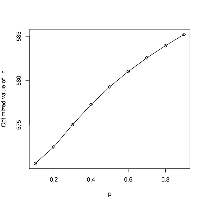
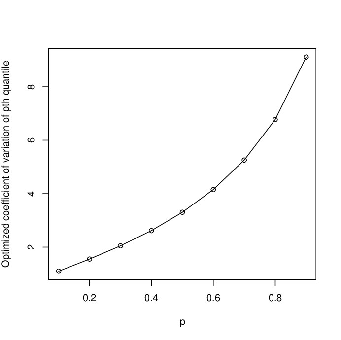
Using these data, one can obtain the ML estimates of the parameters using the likelihood in (2.9) as $\hat{\mu}_{X1}=0.0005$ , $\hat{\mu}_{X2}=0.0007$ , $\hat{\mu}_{Y1}=0.0005$ , $\hat{\mu}_{Y2}=0.0006$ , $\hat{\sigma}_{X}=0.0011$ , $\hat{\sigma}_{Y}=0.0188$ and $\hat{\rho}=0.9422$ .

The optimization process for minimizing $\mbox{Avar}(\hat{\xi}_{p})$ is performed using the optimization procedures of software R.2.14.1. The results including $\hat{\xi}_{p}$ , the optimized approximated coefficient of variation of $\hat{\xi}_{p}$ (minimum C.V.), the optimized time $\tau^{*}$ , the probability of failure under the stress level $S_{1}$ that is $G_{1}(\tau^{*})$ and the probability of failure under the stress level $S_{2}$ , i.e. $G_{2}(C)-G_{2}(\tau^{*})$ , are obtained for $p=0.1(0.1)0.9$ and tabulated in Table 7.

Figure 4 shows the plot of $\tau^{*}$ as a function of $p$ . The values of the optimized approximated coefficient of variation of $\hat{\xi}_{p}$ are also plotted for different values of $p$ in Figure 5. As it can be seen from Figures 4 and 5, the optimal time $\tau^{*}$ is an increasing function of $p$ . It is legal to have such a result, since under a higher stress level the items fail more rapidly and such failures contain more information about lower quantiles of the lifetime distribution of the products. As one can observe from Figure 5, the precision of the optimal estimate of $\hat{\xi}_{p}$ decreases for the upper percentiles of the products’ lifetime distribution.

Acknowledgements

The authors would like to thank two anonymous referees and also Professor M. N. Tata from Shahid Bahonar University and Professor Massoud Amini from Tarbiat Modares University for their valuable comments and suggestion which improved the contents of this paper.

References

[1] Bagdonavicius, V. and Nikulin, M. (2010). Accelerated Life Models: Modeling and Statistical Analysis. Taylor & Francis.
[2] Chhikara R.S. and Folks, J.L. (1989). The Inverse Gaussian Distribution: Theory, Methodology and Applocations. Marcel Dekker: New York.
[3] Cox D.R. and Miller, H.D. (1965). The Theory of Stochastic Processes. John Wiley & Sons: New York.
[4] Jewell, N.P. and Kalbfleisch, J.D. (1996). Marker Processes in Survival Analysis. Lifetime Data Analysis 2:15–29.
[5] Jin, M. (2011). Analysis of Failure Time Data with Mixed-Effects Accelerated Failure Time Model. Communications in Statistics – Simulation and Computation 40:614–619.
[6] Liao, C.M. and Tseng, C.T. (2006). Optimal Design for Step-Stress Accelerated Degradation Tests. IEEE Transactions on Reliability 55:59–66.
[7] Lu, J. (1995). A Reliability Model Based on Degradation and Lifetime Data. Ph.D. Thesis, McGill University, Montreal, Canada.
[8] Nelson, W. (1990). Accelerated Testing: Statistical Models, Test Plans, and Data Analysis. Wiley: New York.
[9] Pan, Z. and Balakrishnan, N. (2010). Multiple Steps Step-Stress Accelerated Degradation Modeling Baesd on Wiener and Gamma Process. Communication in Statistics-Simulation and Computation 39:1384–1402.
[10] Pan, Z., Balakrishnan, N. and Sun, Q. (2011). Bivariate Constant-Stress Accelerated Degradation Model and Inference. Communications in Statistics - Simulation and Computation 40:247–257.
[11] Simino, J., Hollander, M. and McGee, D. (2012). Calibration of Proportional Hazards and Accelerated Failure Time Models. Communications in Statistics – Simulation and Computation 41:922–941.
[12] Tang, L.C., Yang, G.Y. and Xie, M. (2004). Planning of step-stress accelerated degradation test. 2004 Annual Symposium - RAMS. 287-292.
[13] Tseng, S.T., Balakrishnan, N. and Tsai, C.C. (2009). Optimal Step-Stress Accelerated Degradation Test Plan for Gamma Degradation Process. IEEE Transactions on Reliability 58:611–618.
[14] Wang, F. K., Cheng, Y. F. and Lu, W. L. (2012). Partially Accelerated Life Tests for the Weibull Distribution Under Multiply Censored Data. Communications in Statistics - Simulation and Computation 41:1667–1678.
[15] Whitmore, G.A. Crowder, M.J. and Lawless, J.F. (1998). Failure Inference from a Marker Process based on Bivariate Wiener Model, Lifetime Data Analysis 4:229–251.
[16] Yashin, A.I. and Manton, K.G. (1997). Effects of unobserved and partially observed covariate processes on system failure: a review of models and estimation strategies. Statistical Science 12:20–34.

Appendix A. Fisher information matrix

Denoting $\frac{\partial f}{\partial\theta_{r}}$ and $\frac{\partial^{2}f}{\partial\theta_{r}\partial\theta_{s}}$ by $f^{[r]}$ and $f^{[r,s]}$ , respectively, we have

\lambda(y;r,1,0,1)=c_{y}^{[r]},\quad\lambda(y;r,1,1,1)=c_{y}c_{2}^{[r]}(y;1,1),\quad\lambda(y;r,1,0,2)=c_{y}c_{2}^{[r]}(y;1,2),

\lambda(y;r,2,0,1)=c_{y}^{[r]}+\beta_{2}^{[r]}c_{y},\quad\lambda(y;r,2,1,1)=c_{y}c_{2}^{[r]}(y;2,1),\quad\lambda(y;r,2,0,2)=c_{y}c_{2}^{[r]}(y;2,2),

\gamma(y;r,s,1,0,1)=c_{y}^{[r,s]},\quad\gamma(y;r,s,1,1,1)=c_{y}c_{2}^{[r,s]}(1,1)+c_{y}^{[r]}c_{2}^{[s]}(y;1,1)+c_{y}^{[s]}c_{2}^{[r]}(y;1,1),

\gamma(y;r,s,1,0,2)=c_{y}c_{2}^{[r,s]}(y;1,2)+c_{y}^{[r]}c_{2}^{[s]}(y;1,2)+c_{y}^{[s]}c_{2}^{[r]}(y;1,2),

\gamma(y;r,s,k,1,2)=c_{y}[c_{2}^{[r]}(y;k,1)c_{2}^{[s]}(y;k,2)+c_{2}^{[s]}(y;k,1)c_{2}^{[r]}(y;k,2)],\quad k=1,2,

\gamma(y;r,s,k,2,1)=c_{y}c_{2}^{[r]}(y;k,1)c_{2}^{[s]}(y;k,1),\quad\gamma(y;r,s,k,0,3)=c_{y}c_{2}^{[r]}(y;k,2)c_{2}^{[s]}(y;k,2),,\quad k=1,2,

\gamma(y;r,s,2,0,1)=c_{y}^{[r,s]}+\beta_{2}^{[s]}c_{y}^{[r]}+\beta_{2}^{[r]}c_{y}^{[s]}+c_{y}\beta_{2}^{[r]}\beta_{2}^{[s]}+c_{y}\beta_{2}^{[r,s]},

\gamma(y;r,s,2,1,1)=\beta_{2}^{[s]}c_{2}^{[r]}(y;2,1)c_{y}+c_{2}^{[r,s]}(y;2,1)c_{y}+c_{2}^{[r]}(y;2,1)c_{y}^{[s]}+c_{2}^{[s]}(y;2,1)c_{y}^{[r]}+\beta_{2}^{[r]}c_{2}^{[s]}(y;2,1)c_{y},

\gamma(y;r,s,2,0,2)=\beta_{2}^{[s]}c_{2}^{[r]}(y;2,2)c_{y}+c_{2}^{[r,s]}(y;2,2)c_{y}+c_{2}^{[r]}(y;2,2)c_{y}^{[s]}+c_{2}^{[s]}(y;2,2)c_{y}^{[r]}+\beta_{2}^{[r]}c_{2}^{[s]}(y;2,2)c_{y},

Letting $\eta_{4}=\rho(1-\rho^{2})^{-1},\;\eta_{5}=\rho^{-1}+\eta_{4}$ and $\eta_{6}=\rho^{-1}+2\eta_{4},$ we have

c_{y}^{[6]}=-\sigma_{Y}^{-2}c_{y}/2,\;c_{y}^{[6,6]}=3\sigma_{Y}^{-4}c_{y}/4,\;\;c_{y}^{[r,s]}=c_{y}^{[r]}=0,\quad\mbox{for }r\neq 6,\;s\neq 6,

c_{2}^{[1]}(y;1,1)=c_{2}^{[1]}(y;2,1)=-\tau\eta_{3},\;c_{2}^{[2]}(y;1,1)=c_{2}^{[2]}(y;2,1)=-(C-\tau)\eta_{3},

c_{2}^{[3]}(y;1,1)=c_{2}^{[3]}(y;2,1)=\tau\eta_{2}\eta_{3},\;c_{2}^{[4]}(y;1,1)=c_{2}^{[4]}(y;2,1)=(C-\tau)\eta_{2}\eta_{3},

c_{2}^{[5]}(y;1,1)=\eta_{3}\sigma_{X}^{-2}[\eta_{2}q_{2}(C,y)-P_{2}(C)/2],\;c_{2}^{[5]}(y;2,1)=\eta_{3}\sigma_{X}^{-2}[\eta_{2}q_{2}(C,y)-(P_{2}(C)-2D(1-\rho^{2}))/2],

c_{2}^{[6]}(y;1,1)=c_{2}^{[6]}(y;2,1)=-\sigma_{Y}^{-2}\eta_{2}\eta_{3}q_{2}(C,y)/2,

c_{2}^{[7]}(y;1,1)=\eta_{3}[\eta_{4}P_{2}(C)-\eta_{2}\eta_{5}q_{2}(C,y)],\;c_{2}^{[7]}(y;2,1)=\eta_{3}[\eta_{4}P_{2}(C)-\eta_{2}\eta_{5}q_{2}(C,y)+2D\rho],

c_{2}^{[1,5]}(y;1,1)=c_{2}^{[1,5]}(y;2,1)=\frac{\tau}{2}\sigma^{-2}_{X}\eta_{3},\;c_{2}^{[1,7]}(y;1,1)=c_{2}^{[1,7]}(y;2,1)=-\tau\eta_{3}\eta_{4},

c_{2}^{[2,5]}(y;1,1)=c_{2}^{[2,5]}(y;2,1)=\frac{(C-\tau)}{2}\sigma^{-2}_{X}\eta_{3},\;c_{2}^{[2,7]}(y;1,1)=c_{2}^{[2,7]}(y;2,1)=-(C-\tau)\eta_{3}\eta_{4},

c_{2}^{[3,5]}(y;1,1)=c_{2}^{[3,5]}(y;2,1)=-\tau\sigma^{-2}_{X}\eta_{3}\eta_{2},\;c_{2}^{[3,6]}(y;1,1)=c_{2}^{[3,6]}(y;2,1)=\frac{\tau}{2}\sigma^{-2}_{Y}\eta_{3}\eta_{2},

c_{2}^{[3,7]}(y;1,1)=c_{2}^{[3,7]}(y;2,1)=\tau\eta_{3}\eta_{2}\eta_{5},\;c_{2}^{[4,5]}(y;1,1)=c_{2}^{[4,5]}(y;2,1)=-(C-\tau)\sigma^{-2}_{X}\eta_{3}\eta_{2},

c_{2}^{[4,6]}(y;1,1)=c_{2}^{[4,6]}(y;2,1)=\frac{(C-\tau)}{2}\sigma^{-2}_{Y}\eta_{3}\eta_{2},\;c_{2}^{[4,7]}(y;1,1)=c_{2}^{[4,7]}(y;2,1)=(C-\tau)\eta_{3}\eta_{2}\eta_{5},

c_{2}^{[5,5]}(y;1,1)=\eta_{3}\sigma^{-4}_{X}[\frac{3}{4}P_{2}(C)-2\eta_{2}q_{2}(C,y)],\;c_{2}^{[5,5]}(y;2,1)=\eta_{3}\sigma^{-4}_{X}[\frac{3}{4}(P_{2}(C)-2D(1-\rho^{2}))-2\eta_{2}q_{2}(C,y)],

c_{2}^{[5,6]}(y;1,1)=c_{2}^{[5,6]}(y;2,1)=\frac{1}{2}\sigma^{-2}_{X}\sigma_{Y}^{-2}\eta_{3}\eta_{2}q_{2}(C,y),\;c_{2}^{[5,7]}(y;1,1)=\sigma_{X}^{-2}\eta_{3}[\eta_{2}\eta_{5}q_{2}(C,y)-\frac{1}{2}\eta_{4}P_{2}(C)],

c_{2}^{[5,7]}(y;2,1)=\sigma_{X}^{-2}\eta_{3}[\eta_{2}\eta_{5}q_{2}(C,y)-\frac{1}{2}\eta_{4}P_{2}(C)-\rho D],\;c_{2}^{[6,6]}(y;1,1)=c_{2}^{[6,6]}(y;2,1)=\frac{1}{4}\sigma_{Y}^{-4}\eta_{3}\eta_{2}q_{2}(C,y),

c_{2}^{[6,7]}(y;1,1)=c_{2}^{[6,7]}(y;2,1)=-\frac{1}{2}\sigma_{Y}^{-2}\eta_{3}\eta_{2}\eta_{5}q_{2}(C,y),

c_{2}^{[7,7]}(y;1,1)=\eta_{3}[(1+2\rho^{2})(1-\rho^{2})^{-2}P_{2}(C)-3\eta_{2}(1-\rho^{2})^{-2}q_{2}(C,y)],

c_{2}^{[7,7]}(y;2,1)=\eta_{3}[(1+2\rho^{2})(1-\rho^{2})^{-2}P_{2}(C)-3\eta_{2}(1-\rho^{2})^{-2}q_{2}(C,y)+2D(1-\rho^{2})^{-1}],

and $c_{2}^{[r,s]}(y;1,1)=c_{2}^{[r,s]}(y;2,1)=0$ otherwise $r,s$ . Also,

c_{2}^{[3]}(y;1,2)=c_{2}^{[3]}(y;2,2)=-\tau c_{y},\;c_{2}^{[4]}(y;1,2)=c_{2}^{[4]}(y;2,2)=-(C-\tau)c_{y},

c_{2}^{[5]}(y;1,2)=0,\;c_{2}^{[5]}(y;2,2)=D\rho C^{-1/2}\sigma_{X}^{-3},

c_{2}^{[6]}(y;1,2)=c_{2}^{[6]}(y;2,2)=-\frac{1}{2}\sigma_{Y}^{-2}q_{2}(C,y)c_{y},\;c_{2}^{[7]}(y;1,2)=0,\;c_{2}^{[7]}(y;2,2)=-2DC^{-1/2}\sigma_{X}^{-1},

c_{2}^{[r]}(y;1,2)=c_{2}^{[r]}(y;2,2)=0,\;r=1,2,

c_{2}^{[3,6]}(y;1,2)=c_{2}^{[3,6]}(y;2,2)=\frac{\tau}{2}\sigma^{-2}_{Y}c_{y},\;c_{2}^{[4,6]}(y;1,2)=c_{2}^{[4,6]}(y;2,2)=\frac{(C-\tau)}{2}\sigma^{-2}_{Y}c_{y},

c_{2}^{[5,5]}(y;1,2)=0,\;c_{2}^{[5,5]}(y;2,2)=-\frac{3}{2}D\sigma_{X}^{-5}C^{-1/2}\rho,\;c_{2}^{[5,7]}(y;1,2)=0,\;c_{2}^{[5,7]}(y;2,2)=D\sigma_{X}^{-3}C^{-1/2},

c_{2}^{[6,6]}(y;1,2)=c_{2}^{[6,6]}(y;2,2)=\frac{3}{4}\sigma_{Y}^{-4}q_{2}(C,y)c_{y},

and $c_{2}^{[r,s]}(y;1,2)=c_{2}^{[r,s]}(y;2,2)=0$ otherwise $r,s$ . Furthermore

\beta_{2}^{[1]}=2D\tau\sigma_{X}^{-2}C^{-1},\;\beta_{2}^{[2]}=2D(C-\tau)\sigma_{X}^{-2}C^{-1},\;\beta_{2}^{[5]}=-2D(D-P_{2}(C))\sigma_{X}^{-4}C^{-1},

\beta_{2}^{[r]}=0,\;r=3,4,6,7,

\beta_{2}^{[1,5]}=-2D\tau\sigma_{X}^{-4}C^{-1},\;\beta_{2}^{[2,5]}=-2D(C-\tau)\sigma_{X}^{-4}C^{-1},\;\beta_{2}^{[5,5]}=4D(D-P_{2}(C))\sigma_{X}^{-6}C^{-1},

and $\beta_{2}^{[r,s]}=0,$ otherwise $r,s$ .

\alpha_{5,5}=-\frac{1}{2\sigma_{X}^{4}},\;\alpha_{6,6}=-\frac{1}{2\sigma_{Y}^{4}},\;\alpha_{7,7}=-\frac{(1+\rho^{2})}{(1-\rho^{2})^{2}},\;\alpha_{r,s}=0

otherwise $r,s$ . Also, for $j=1,2,$

\zeta_{j}(1,1)=(1-\rho^{2})^{-1}\sigma_{X}^{-2}{\rm E}(T^{3-2j})\tau^{2j-2},\;\zeta_{1}(1,2)=0,\;\zeta_{2}(1,2)=(1-\rho^{2})^{-1}\sigma_{X}^{-2}\tau(1-\tau{\rm E}(T^{-1})),

\zeta_{j}(1,3)=-2\eta_{1}\eta_{2}{\rm E}(T^{3-2j})\tau^{2j-2},\;,\zeta_{1}(1,4)=0,\;\zeta_{2}(1,4)=-2\eta_{1}\eta_{2}\tau(1-\tau{\rm E}(T^{-1})),

\zeta_{j}(1,5)=\frac{1}{2}\sigma_{X}^{-4}(1-\rho^{2})^{-1}[2{\rm E}(T^{1-j}P_{j}(T))-\rho\sigma_{X}\sigma_{Y}^{-1}{\rm E}_{P_{f_{j}}}(T^{1-j}q_{j}(T,Y))]\tau^{j-1},

\zeta_{j}(1,6)=-\sigma_{Y}^{-2}\eta_{1}\eta_{2}{\rm E}_{P_{f_{j}}}(T^{1-j}q_{j}(T,Y))\tau^{j-1},

\zeta_{j}(1,7)=2\eta_{2}\eta_{1}[\eta_{6}{\rm E}_{P_{f_{j}}}(T^{1-j}q_{j}(T,Y))-2\eta_{2}\eta_{4}{\rm E}(T^{1-j}P_{j}(T))]\tau^{j-1},

\zeta_{1}(2,2)=\zeta_{1}(2,3)=\cdots=\zeta_{1}(2,7)=0,

\zeta_{2}(2,2)=(1-\rho^{2})^{-1}\sigma_{X}^{-2}{\rm E}(T^{-1}(T-\tau)^{2}),\;\zeta_{2}(2,3)=-2\eta_{1}\eta_{2}\tau(1-\tau{\rm E}(T^{-1})),

\zeta_{2}(2,4)=-2\eta_{1}\eta_{2}{\rm E}(T^{-1}(T-\tau)^{2}),

	$\displaystyle\zeta_{2}(2,5)$	$\displaystyle=$	$\displaystyle\frac{1}{2}\sigma_{X}^{-4}(1-\rho^{2})^{-1}[2({\rm E}(P_{2}(T))-\tau{\rm E}(T^{-1}P_{2}(T)))$
			$\displaystyle-\rho\sigma_{X}\sigma_{Y}^{-1}({\rm E}_{P_{f_{2}}}(q_{2}(T,Y))-\tau{\rm E}_{P_{f_{2}}}(T^{-1}q_{2}(T,Y)))],$

\zeta_{2}(2,6)=-\sigma_{Y}^{-2}\eta_{1}\eta_{2}({\rm E}_{P_{f_{2}}}(q_{2}(T,Y))-\tau{\rm E}_{P_{f_{2}}}(T^{-1}q_{2}(T,Y))),

	$\displaystyle\zeta_{2}(2,7)$	$\displaystyle=$	$\displaystyle 2\eta_{2}\eta_{1}[\eta_{6}({\rm E}_{P_{f_{j}}}(q_{j}(T,Y))-\tau{\rm E}_{P_{f_{j}}}(T^{-1}q_{j}(T,Y)))$
			$\displaystyle-2\eta_{2}\eta_{4}({\rm E}(P_{j}(T))-\tau{\rm E}(T^{-1}P_{j}(T)))],$

\zeta_{j}(3,3)=2\eta_{1}{\rm E}(T^{3-2j})\tau^{2j-2},

\zeta_{1}(3,4)=0,\;\zeta_{2}(3,4)=2\eta_{1}\tau(1-\tau{\rm E}(T^{-1})),\;\zeta_{j}(3,5)=-\sigma_{X}^{-2}\eta_{2}\eta_{1}{\rm E}(T^{1-j}P_{j}(T))\tau^{j-1},

\zeta_{j}(3,6)=\sigma_{Y}^{-2}\eta_{1}[2{\rm E}_{P_{f_{j}}}(T^{1-j}q_{j}(T,Y))-\eta_{2}{\rm E}(T^{1-j}P_{j}(T))]\tau^{j-1},

\zeta_{j}(3,7)=2\eta_{1}[\eta_{2}\eta_{6}{\rm E}(T^{1-j}P_{j}(T))-2\eta_{4}{\rm E}_{P_{f_{j}}}(T^{1-j}q_{j}(T,Y))]\tau^{j-1},

\zeta_{1}(4,4)=\zeta_{1}(4,5)=\zeta_{1}(4,6)=\zeta_{1}(4,7)=0,\;\zeta_{2}(4,4)=2\eta_{1}{\rm E}(T^{-1}(T-\tau)^{2}),

\zeta_{2}(4,5)=-\sigma_{X}^{-2}\eta_{2}\eta_{1}({\rm E}(P_{2}(T))-\tau{\rm E}(T^{-1}P_{2}(T))),

\zeta_{2}(4,6)=\sigma_{Y}^{-2}\eta_{1}[2({\rm E}_{P_{f_{2}}}(q_{2}(T,Y))-\tau{\rm E}_{P_{f_{2}}}(T^{-1}q_{2}(T,Y)))-\eta_{2}({\rm E}(P_{2}(T))-\tau{\rm E}(T^{-1}P_{2}(T)))],

\zeta_{2}(4,7)=2\eta_{1}[\eta_{2}\eta_{6}({\rm E}(P_{2}(T))-\tau{\rm E}(T^{-1}P_{2}(T)))-2\eta_{4}({\rm E}_{P_{f_{2}}}(q_{2}(T,Y))-\tau{\rm E}_{P_{f_{2}}}(T^{-1}q_{2}(T,Y)))],

\zeta_{j}(5,5)=\sigma_{X}^{-4}\eta_{1}\eta_{2}[2\eta_{2}{\rm E}(T^{-1}P_{j}^{2}(T))-3{\rm E}_{P_{f_{j}}}(T^{-1}P_{j}(T)q_{j}(T,Y)))/2]+\sigma_{X}^{-6}{\rm E}(T^{-1}P_{j}^{2}(T)),

\zeta_{j}(5,6)=\frac{-1}{2}\sigma_{X}^{-2}\sigma_{Y}^{-2}\eta_{1}\eta_{2}{\rm E}_{P_{f_{j}}}(T^{-1}P_{j}(T)q_{j}(T,Y))),

\zeta_{j}(5,7)={\sigma_{X}^{-2}}\eta_{1}\eta_{2}[\eta_{6}{\rm E}_{P_{f_{j}}}(T^{-1}P_{j}(T)q_{j}(T,Y)))-2\eta_{5}\eta_{2}{\rm E}(T^{-1}P_{j}^{2}(T))],

\zeta_{j}(6,6)=\eta_{1}\sigma_{Y}^{-4}[2{\rm E}_{P_{f_{j}}}(T^{-1}q_{j}^{2}(T,Y)))-\frac{3}{2}\eta_{2}{\rm E}_{P_{f_{j}}}(T^{-1}P_{j}(T)q_{j}(T,Y)))],

\zeta_{j}(6,7)=-\eta_{1}\sigma_{Y}^{-2}[2\eta_{4}{\rm E}_{P_{f_{j}}}(T^{-1}q_{j}^{2}(T,Y)))-\eta_{2}\eta_{6}{\rm E}_{P_{f_{j}}}(T^{-1}P_{j}(T)q_{j}(T,Y)))],

	$\displaystyle\zeta_{j}(7,7)$	$\displaystyle=$	$\displaystyle 2\eta_{1}\eta_{4}^{2}((3+\rho^{-2}){\rm E}_{P_{f_{j}}}(T^{-1}q_{j}^{2}(T,Y)))+(3\rho^{-2}+\rho^{-4})(\eta_{2}{\rm E}(T^{-1}P_{j}^{2}(T)))$
			$\displaystyle-2(1+3\rho^{-2})\eta_{2}{\rm E}_{P_{f_{j}}}(T^{-1}P_{j}(T)q_{j}(T,Y)))).$