Distributed Scheduling Algorithms for Crosspoint-Buffered Switches

A sequence of random variables ($X_{0}$, $X_{1}$, $\cdots$) is a Markov chain with state space ${\bf\Omega}$ and transition matrix ${\bf P}$ if for all $x$, $y\in{\bf\Omega}$, all $n\geq 1$, and all events $\textrm{ $\mathcal{H}$}_{n-1}$$=\cup_{s=0}^{n-1}{\{X_{s}=x_{s}\}}$, we have

The process can then be described as:

where $\mu$$(\tau)$ is the probability distribution of $X_{\tau}$.

The Markov chain is irreducible if any state can reach any other state. If the system starts from any state $X$ and it can return to the state within finite time with a probability $1$, the Markov chain is positive recurrent. If the Markov chain is irreducible and positive recurrent, it has a unique stationary distribution $\pi$ so that:

Let $P^{*}$ denote the transition probability matrix for the reverse Markov chain ($\cdots,X_{n},X_{n-1},\cdots$). If $P=P^{*}$, the Markov chain is called time-reversible [24].

A graph $G=(V,E)$ consists of a vertex set $V$ and an edge set $E$, where the elements of $E$ are unordered pair of vertices: $E\subset\{\{x,y\}:x,y\in V,x\neq y\}$. If $\{x,y\}\in E$, $y$ is a neighbor of $x$ (and also $x$ is a neighbor of $y$). Let $\mathcal{N}(x)$ denote all the neighbors of $x$. A independent set $I\subset V$ is a set such that if $x\in I$, $\forall y\in\mathcal{N}(x)$, $y\notin I$. Let $\mathcal{I}(G)$ represent all the independent sets of $G$.

The Glauber dynamics is irreducible, aperiodic and time-reversible over $\mathcal{I}(G)$ [24]. It has a product-form stationary distribution, which is:

where $Z$ is a normalizing constant in order to have the sum of the probabilities have unit total mass.

Glauber dynamics can converge to its stationary distribution starting from any initial distribution. To characterize the convergence speed, we need to quantify the time that it takes for Glauber dynamics to reach close to its stationary distribution. To establish the result, we need to define some notations first.

Following [25], we have the following condition:

From the definition, we can see that mixing time is a parameter to measure the convergence rate of a Markov chain to its stationary distribution. Also, following Eqn 5, the mixing time can be measured by calculating the $\chi^{2}$ distance of $\textrm{\boldmath$\mu$}(\tau)$ and $\pi$ .

With today’s ASIC technology, it is now possible to add a small buffer at each crosspoint inside the crossbar (see Fig. 1). This makes the crosspoint buffered or combined input and crossbar queueing (CICQ) switch a much more attractive architecture since its scheduler is potentially much simpler. The input and output schedulers can be independent. First, each input picks a crosspoint buffer to send a packet to. Then, each output picks a crosspoint buffer to transmit a packet from. However, existing algorithms [12, 13, 26, 27] either cannot guarantee $100\%$ throughput or require a centralized scheduler.

An $N\times N$ crosspoint buffered switch is shown in Fig. 1. We assume fixed size packet (cell) switching. Variable size packets can be segmented into cells before switching and reassembled at the output ports. There are virtual output queues (VOQs) at the inputs to prevent head-of-line blocking. Each input maintains $N$ VOQs, one for each output. Let $VOQ_{ij}$ represent the VOQ at input $i$ for output $j$, and $Q_{ij}(n)$ the queue length of $VOQ_{ij}$ at time $n$. Let $(i,j)$ represent the crosspoint between input $i$ and output $j$.

Each crosspoint has a buffer of size $K$. Most current implementations are constrained by the buffer size. However, it turns out that $K=1$ is sufficient for DISQUO. We will therefore assume that $K=1$ in the following. Our algorithm can be easily extended to the case when $K>1$. Let $CB_{ij}$ denote the buffer at the crosspoint between input $i$ and output $j$. $B_{ij}(n)$ $\in$ $\{0,1\}$ denotes the occupancy of $CB_{ij}$ at time $n$.

A schedule can be represented by S(n) = $[\textbf{S}^{I}(n),\textbf{S}^{O}(n)]$. $\textbf{S}^{I}(n)=[S^{I}_{ij}(n)]$ is the input schedule. Each input port can only transmit at most one cell at each time slot. Thus the input schedule is subject to the following constraints:

$\textbf{S}^{O}(n)=[S^{O}_{ij}(n)]$ is the output schedule. It has to satisfy the following constraints:

Let $\lambda_{ij}$ represent the arrival rate of traffic between input $i$ and output $j$. We assume that the arrival process is i.i.d. Bernoulli.

Let $\textrm{\boldmath$\sigma$}^{*}$ denote the traffic that the equivalence in Eq. (10) holds. It is easy to verify that for any admissible traffic $\sigma$, there exists an $\epsilon>0$ such that $\textrm{\boldmath$\sigma$}<(1-\epsilon)\textrm{\boldmath$\sigma$}^{*}$ component-wise.

Let $||{\bf Q}||$ represent the norm of matrix Q: $||{\bf Q}||=\big(\sum_{i,j}{Q_{ij}^{2}}\big)^{1/2}$. The stability of a system is defined as:

Before presenting the algorithm, we need to introduce some further notation. A DISQUO schedule ${\bf X}(n)$ is a schedule that is generated by the DISQUO algorithm. It is used to determine the input schedules and output schedules. A DISQUO schedule has the following properties:

With some abuse of notation, we also use ${\bf X}$ to represent a set, and write $(i,j)$ $\in$ ${\bf X}$ if $X_{ij}=1$. Note that a DISQUO schedule X has the property that if $X_{ij}=1$, then $\forall i^{\prime}\neq i$, $X_{i^{\prime}j}=0$ and $\forall j^{\prime}\neq j$, $X_{ij^{\prime}}=0$. We define these crosspoints as its neighbors as follows.

A DISQUO schedule X then has the following property:

Let $\mathcal{X}$ represent the set of all DISQUO schedules.

Following Prop. 3-5, the input schedule ${\bf S}^{I}(n)$ and output schedule ${\bf S}^{O}(n)$ can be determined after the DISQUO schedule ${\bf X}(n)$ is generated.

As shown in the Glauber dynamics, ${\bf X}(n)$ is generated based on ${\bf X}(n-1)$. Therefore, each input $i$ needs to keep track of the DISQUO schedule in the previous slot, i.e. for which output $j$ was $X_{ij}(n-1)=1$. Similarly, each output needs to keep track of for which input $i$ was $X_{ij}(n-1)=1$. Since the algorithm is distributed, there is no message passing between inputs and outputs. DISQUO needs to make sure that the inputs and outputs keep a consistent view of the DISQUO schedule. For example, if $X_{ij}(n)=1$, both input $i$ and output $j$ should be aware of this.

Since the decision for a crosspoint to join or leave the DISQUO schedule needs the queue length information, inputs are responsible for making the decisions. However, there are two problems that have to be solved: 1) before input $i$ decides to change $X_{ij}$ from $0$ to $1$, it needs to check the states of all the neighbors of $(i,j)$, namely, the status of output $j$, which is not directly accessible at input $i$; 2) after input $i$ changes the value of $X_{ij}$, this information has to be passed over to output $j$. To solve these problems, the DISQUO algorithm is designed to achieve implicit message passing by utilizing the crosspoint buffers.

At the beginning, set the initial DISQUO schedule ${\bf X}(0)$ to any schedule that satisfies Property 1. For simplicity, we can set ${\bf X}(0)=\emptyset$. At the beginning of each time slot $n$, generate an input/output permutation ${\bf H}(n)$ randomly. To this purpose, we can use a pseudo-random number generator, using the same seed at all ports. Then each port will generate the same random schedule ${\bf H}(n)$. Then, the DISQUO algorithm works as follows:

In the algorithm, $p_{ij}$ is defined as: $p_{ij}=\frac{\exp(W_{ij}(n))}{1+\exp(W_{ij}(n))}$, where $W_{ij}(n)$ is a weight function of the queue size $Q_{ij}(n)$, which is defined as

$f(\cdot)$ is a concave function which we will define later, $Q_{max}(n)=\max_{i,j}{Q_{ij}(n)}$, and $\tilde{Q}_{ij}(n)=\max\{f^{-1}(\frac{\epsilon}{2N^{2}}f(Q_{max}(n))),Q_{ij}(n)\}$. Recall that for any admissible traffic $\sigma$, there exists an $\epsilon>0$ such that $\textrm{\boldmath$\sigma$}<(1-\epsilon)\textrm{\boldmath$\sigma$}^{*}$ component-wise. Thus, $\epsilon$ is a small positive number that satisfies the condition $\textrm{\boldmath$\sigma$}<(1-\epsilon)\textrm{\boldmath$\sigma$}^{*}$.

Note that in our algorithm, $X_{ij}(n)$ can change only when $(i,j)$ is in ${\bf H}(n)$. Therefore, at every time slot, only $(i,j)\in{\bf H}(n)$ can join or leave the DISQUO schedule.

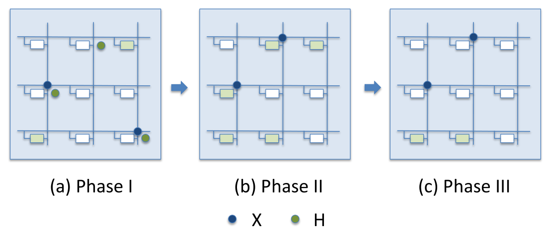
To help understand DISQUO, we give an illustrative example here. We assume that in one time slot, a crosspoint buffer can have one write and one read, i.e., input $i$ can transmit a packet to buffer $CB_{ij}$, and then output $j$ can get the packet from the buffer. Then a schedule over one time slot can be divided into three phases: a) Phase I: every input and output calculate the same random schedule ${\bf H}(n)$; b) Phase II: inputs update the DISQUO schedule based on ${\bf H}(n)$, and decide the value of ${\bf S}^{I}(n)$, after which packets can be sent from inputs to the crosspoint buffers; c) Phase III: outputs update the DISQUO schedule and decide the value of ${\bf S}^{O}(n)$ so that they can transmit packets from the crosspoint buffers.

As we can see from Fig. 2(a), the DISQUO schedule at time $n-1$ is ${\bf X}(n-1)=\{(2,1),(3,3)\}$. In Phase I, $\textbf{H}(n)$ = $\{(1,2),(2,1),(3,3)\}$ is generated at each input and output. In the following, we use the example to describe how a crosspoint joins or leaves the DISQUO schedule, and how the input/output scheduler ${\bf S}^{I}(n)$ and ${\bf S}^{O}(n)$ are decided after ${\bf X}(n)$ is generated.

• •

  How a crosspoint joins the DISQUO schedule: $(1,2)$ is in ${\bf H}(n)$ and $X_{12}(n-1)=0$. Also, input $1$ knows that $\forall j$, $X_{1j}(n-1)=0$ so that input 1 was a free input in the previous slot. If output $2$ was also a free output, input $1$ can decide whether to let $(1,2)$ join the DISQUO schedule or not, following case (e) or (f) of ISA. Input $1$ cannot know the status of output $2$ directly. However, it can learn output $2$’s status by observing $CB_{12}$. Since $CB_{12}$ is empty, input $i$ learns that output $2$ was free. It can then decide whether to make $(1,2)$ active based on $p_{12}$. If its decision is to set $X_{12}(n)$ to $1$, it should send a packet to $CB_{12}$. Otherwise, it remains a free input. In the example, the decision of input $1$ is to set $X_{12}(n)$ to $1$. Thus, $S^{I}_{12}(n)=1$, and it sends a packet to $CB_{12}$, as shown in Fig. 2(b). Note that this transmission implicitly passes its decision information to output $2$.

  Output $2$ was a free output, and it observes that in Phase II, input $1$ sends a packet to $CB_{12}$. Following case (e) of OSA, output $2$ learns input $1$’s decision of setting $X_{12}(n)$ to $1$. It then updates $X_{12}(n)$ to $1$, and thus $S^{O}_{12}(n)=1$. Output $2$ transmits the packet from $CB_{12}$, which is shown in Fig. 2(c).

• •

  How a crosspoint leaves the DISQUO schedule: $(3,3)$ is in ${\bf H}(n)$ and $X_{33}(n-1)=1$. Following case (b) and (c), input $3$ has to decide whether to keep $(3,3)$ in the DISQUO schedule or not, based on a probability $p_{33}$ which is a function of the queue size $Q_{33}$. In the example, it decides to set $X_{33}(n)$ to $0$. Input $3$ becomes a free input. It calculates ${\bf H}(n+1)$, which we assume is $\{(1,3),(2,1),(3,2)\}$. Since $(3,2)\in{\bf H}(n+1)$ and $CB_{32}$ is empty, it sets $S^{I}_{32}(n)=1$, and sends a packet to $CB_{32}$ (Fig. 2(b)). Note that by not sending a packet to $CB_{33}$, input $3$ implicitly passes its decision of setting $X_{33}(n)=0$ to output $3$.

  Output 3 observes that, in Phase II, input $3$ did not send any packet to $CB_{33}$. Following case (c) of OSA, it learns input $3$’s decision and updates $X_{33}(n)$ to $0$. Output $3$ becomes a free output. Following the OSA, a free output has to generate ${\bf H}(n+1)$ at time $n$. Since $(1,3)\in{\bf H}(n+1)$ and $CB_{13}$ is not empty, output $3$ sets $S^{O}_{13}(n)=1$ and transmits the packet from $CB_{13}$, as shown in Fig. 2(c).

From the example, we can see that, after ${\bf X}(n)$ is generated, which is $\{(1,2),(2,1)\}$, a packet is transmitted from input $1$ to output $2$, and one from input $2$ to output $1$. Besides that, input $3$ and output $3$, which are free, also transmit a packet. The transmissions by free inputs and outputs can be considered as an augmentation of ${\bf X}(n)$. In the following, we will show that the weight, only defined on ${\bf X}(n)$, is close enough to the maximum one to guarantee the throughput. The augmenting by free inputs or outputs, though it does not contribute to the stability of the switch, can improve the delay performance of the system.

As presented in the previous section, the decision of making a crosspoint $(i,j)$ active or not is based on a probability $p_{ij}$, which depends on not only the local queue sizes, but also a global information $Q_{max}(n)$. However, since $\frac{\epsilon}{2N^{2}}$ is very small, we can use $W_{ij}(n)=f(Q_{ij}(n))$ directly for implementation. The introduction of $Q_{max}(n)$ is primarily for technical reasons. Therefore, we have the following conjecture.

To be precise, for provable stability we still need some message passing between linecards. As suggested in [18, 25], a rough estimate of $Q_{max}(n)$ is sufficient to guarantee the convergence of the system. Therefore, a relatively low-rate Ethernet connection, which is typical in current router design for backplane control, can be used for linecards to broadcast their local maximum queue sizes so that other linecards estimate the value of $Q_{max}(n)$. At time slot $kN+i$, only linecard $i$ broadcasts its local maximum queue size. Since at every time slot, there is at most one packet departure/arrival from/to an input, the estimation of ${Q}_{max}(n)$, denoted as $\tilde{Q}_{max}(n)$, satisfies: $Q_{max}(n)-2N\leq\tilde{Q}_{max}(n)\leq{Q}_{max}(n)+2N$. This is sufficient for the system stability. For details, please refer to Ref. [18, 25].

Note that we assume there is no delay between the linecards and the crosspoint buffers. For large-scale switches, this delay is not negligible. One way to address this issue is to use a frame-like schedule, i.e., instead of generating a DISQUO schedule in each time slot, we can generate the DISQUO schedule in $N$ time slots, where $N$ is the delay [27].

As mentioned before, $\{{\bf X}(n)\}$ forms a Markov chain. In this section, we will derive the stationary distribution of this Markov chain, and show that after the system converges, the weight of the DISQUO schedule approaches the weight of the MWM schedule (in Lemma 8). We can then prove the system stability in Theorem 2.

For Glauber dynamics, the weights are fixed over time. Therefore, the convergence rate of the system can be described by the distance between $\mu$(n) and $\pi$. However, following the algorithm presented in the previous section, the weights are changing over time such that the Glauber dynamics for each time slot $n$ is different from those in other time slots, which means $\textrm{\boldmath$\pi$}_{n}$ also varies over time. To characterize the convergence rate of this system, we can use the distance definition in Definition 2

We aim to ensure that for any arbitrarily small $\delta>0$, there exists a time $T_{mix}(\delta)$ that for any $n>T_{mix}(\delta)$, we have $d_{n}<\delta$ so that $\textrm{\boldmath$\mu$}_{n}$ and $\textrm{\boldmath$\pi$}_{n}$ are close enough. As compared to the definition of mixing time in Definition 3, $T_{mix}(\delta)$ shows the convergence rate of the system. Therefore, we will refer to $T_{mix}(\delta)$ as the mixing time of this inhomogeneous Markov chain.

In the following Lemma, we will prove that if the weight function $f(x)$, so that $W_{ij}(n)=f(Q_{ij}(n))$ , is carefully selected, the system can always converge to the distribution $\textrm{\boldmath$\pi$}_{n}$ by following the DISQUO scheduling algorithm.

As shown above, the Markov chain $\{{\bf X}(n)\}$ has a finite number of states, and we already derived its stationary distribution. In the following, we will use the MWM algorithm to prove the system stability. For an input-queued switch, the MWM algorithm selects a feasible schedule ${\bf S}(n)$ with the maximum weight:

The algorithm can provide $100\%$ throughput for any admissible traffic in a bufferless crossbar switch [5]. According to Theorem 1, MWM can be extended to a buffered crossbar switch. Following the DISQUO algorithm, if $X_{ij}(n)=1$, and $Q_{ij}(n)>0$ or $B_{ij}(n)>0$, one packet can be transmitted from input $i$ to output $j$. Therefore, we can define the weight of a DISQUO schedule as:

For MWM, the result below has been established in [29].

References

- [1] R. Hemenway, R. Grzybowski, C. Minkenberg, and R. Luijten, “Optical- packet-switched Interconnect for Supercomputer Applications,” Journal of Optical Networks, vol. 3, no. 12, pp. 900–913, 2004.
- [2] C. Minkenberg, F. Abel, R. Krishnamurthy, M. Gusat, P. Dill, I. Iliadis, R. Luijten, B. R. Hemenway, R. Grzybowski, and E. Schiattarella, “Designing a Crossbar Scheduler for HPC Applications,” IEEE Micro, vol. 26, pp. 58–71, May-June 2006.
- [3] M. Al-Fares, A. Loukissas, and A. Vahdat, “A Scalable, Commodity, Data Center Network Architecture,” in Proceedings of ACM SIGCOMM, August 2008.
- [4] N. Farrington, G. Porter, S. Radhakrishnan, H. H. Bazzaz, V. Subramanya, Y. Fainman, G. Papen, and A. Vahdat, “Helios: A Hybrid Electrical/Optical Switch Architecture for Modular Data Centers,” in Proceedings of ACM SIGCOMM, Aug-Sep 2010.
- [5] L. Tassiullas and A. Ephremides, “Stability Properties of Constrained Queuing Systems and Scheduling Policies for Maximum Throughput in Multihop Radio Networks,” IEEE Transactions on Automatic Control, vol. 37, pp. 1936–1949, December 1992.
- [6] N. McKeown, A. Mekkittikul, V. Anantharam, and J. Walrand, “Achieving Throughput in an Input-Queued Switch,” IEEE Transactions on Communications, vol. 47, pp. 1260–1267, August 1999.
- [7] N. Mckeown, “The iSLIP Scheduling Algorithm for Input-Queued Switches,” IEEE/ACM Transactions on Networking, vol. 7, pp. 188–201, April 1999.
- [8] Y. Li, S. Panwar, and H. J. Chao, “On the Performance of a Dual Round-Robin Switch,” in Proc. of IEEE INFOCOM, April 2001.
- [9] T. E. Anderson, S. S. Owichi, J. B. Saxe, and C. P. Thacher, “High Speed Switch Scheduling for Local Area Networks,” ACM Transactions on Computer Systems, vol. 11, pp. 319–352, November 1993.
- [10] J. G. Dai and B. Prabhakar, “The Throughput of Data Switches with and without Speedup,” in Proceedings of IEEE INFOCOM, (Tel Aviv, Israel), 2000.
- [11] S. Chuang, A. Goel, N. McKeown, and B. Prabhakar, “Matching Output Queueing with a Combined Input Output Queued Switch,” in Proc. of IEEE INFOCOM, March 1999.
- [12] R. Rojas-Cessa, E. Oki, and H. J. Chao, “On the Combined Input-Crosspoint Buffered Packet Switch with Round-Robin Arbitration,” IEEE Transactions on Communications, vol. 53, pp. 1945–1951, November 2005.
- [13] T. Javidi, R. Magill, and T. Hrabik, “A High Throughput Scheduling Algorithm for a Buffered Crossbar Switch Fabric,” in Proceedings of IEEE ICC, (Helsinki, Finland), June 2001.
- [14] L. Mhamdi and M. Hamdi, “MCBF: a High-Performance Scheduling Algorithm for Buffered Crossbar Switches,” IEEE Communications Letters, vol. 7, pp. 451–453, September 2003.
- [15] S.-T. Chuang, S. Iyer, and N. McKeown, “Practial Algorithms for Performance Guarantees in Buffered Crossbars,” in Proceedings of IEEE INFOCOM, (Miami, Florida), March 2005.
- [16] J. Turner, “Strong Performance Guarantees for Asynchronous Crossbar Schedulers,” in Proceedings of IEEE INFOCOM, (Spain), April 2006.
- [17] P. Giaccone, E. Leonardi, and D. Shah, “On th emaximal throughput of networks with finite buffers and its application to buffered crossbars,” in Proceedings of IEEE Infocom, (Miami, FL), March 2005.
- [18] S. Rajagopalan, D. Shah, and J. Shin, “Network adiabatic theorem: an efficient randomized protocol for contention resolution,” in Proceedings of ACM SIGMETRICS, June 2009.
- [19] L. Jiang and J. Walrand, “A Distributed CSMA Algorithm for Throughput and Utility Maximization in Wireless Networks,” IEEE/ACM Transactions on Networking, vol. 18, pp. 960–972, June 2010.
- [20] J. Ni and R. Srikant, “Q-CSMA: Queue-Length Based CSMA/CA Algorithms for Achieving Maximum Throughput and Low Delay in Wireless Networks,” Proceedings of IEEE Infocom, Apr. 2010.
- [21] J. Liu, Y. Yi, A. Proutiére, M. Chiang, and H. V. Poor, “Towards utility-optimal random access without message passing,” Wireless Communications and Mobile Computing, vol. 10, pp. 115–128, Jan. 2010.
- [22] L. Jiang, M. Leconte, J. Ni, R. Srikant, and J. Walrand, “Fast Mixing of Parallel Glauber Dynamics and Low-Delay CSMA Scheduling,” submitted, August 2010.
- [23] J. Ghaderi and R. Srikant, “On the Design of Efficient CSMA Algorithms for Wireless Networks,” submitted, 2010.
- [24] D. A. Levin, Y. Peres, and E. L. Wilmer, Markov Chains and Mixing Times. American Mathematical Society, 2009.
- [25] S. Rajagopalan and D. Shah, “Aloha that works,” submitted, Nov. 2008.
- [26] Y. Shen, S. S. Panwar, and H. J. Chao, “Providing Throughput in a Buffered Crossbar Switch,” in Proceedings of IEEE HPSR, (Brooklyn, New York), May-June 2007.
- [27] Y. Shen, S. S. Panwar, and H. J. Chao, “SQUID: A Practical 100Scheduler for Crosspoint Buffered Switches,” IEEE/ACM Transactions on Networking, vol. 18, pp. 1119–1131, August 2010.
- [28] F. Kelly, Reversibility and Stochastic Networks. Wiley, 1979.
- [29] A. Eryilmaz, R. Srikant, and J. R. Perkins, “Stable Scheduling Policies for Fading Wireless Channels,” IEEE/ACM Transactions on Networking, vol. 13, pp. 411–424, April 2005.
- [30] S. Ye, Distributed Scheduling Algorithm Design for High Speed Switching Systems. PhD thesis, Polytechnic Institute of New York University, 2011.
- [31] M. Jerrum and A. Sinclair, “Approximating the permanent,” SIAM Journal of Computing, vol. 18, pp. 1149–1178, 1989.
- [32] P. Bremaud, Markov chains, Gibbs fields, Monte Carlo simulation and queues. Springer-Verlag, 2001.
-A Proof of Lemma 2
Proof:
The transition occurs only when the VOQs in H satisfy the conditions below:
- 1.
For any : the VOQ is selected by H and decides to change its scheduling decision from to , which happens with probability .
- 2.
- 3.
For any : the VOQ was in the DISQUO schedule of the previous time slot, and even though selected by H it decides to keep its state, which occurs with probability .
- 4.
For any : neither the VOQ nor any of its neighbors was in the DISQUO schedule of the previous time slot, and though selected by H it decides to keep its schedule, which occurs with probability . Since H is a DISQUO schedule and , . Thus = . We replace by in Eq. (2) for the proof of the stationary distribution in the following.
Since H is a permutation of the inputs and outputs, for any two VOQs in H, they are not neighbors of each other. Therefore, they can make the scheduling decisions independently. We can then multiply the probabilities of all the four categories above, which leads to the transition probability given by Eq. (2). ∎
-B Proof of Lemma 3
Suppose that X is a DISQUO schedule, and it has non-zero elements: , X. Let represent a DISQUO schedule which has non-zero elements: , X, . We can see that and . Since X is a DISQUO schedule, is also a DISQUO schedule and . Therefore, the system can make a transition from to with positive probability when , as we already proved in Lemma 2. Hence, state can reach any state X with positive probability in a finite number of steps and vice versa. Thus, the Markov chain is irreducible and positive recurrent. ∎
-C Lemmas for System Stability
Lemma 7.
Suppose that is a function defined on a set . For any probability distribution on , define the function: