Scaled pier fractals do not strictly self-assemble

This work is an extension of the conference paper titled, “Scaled tree fractals do not strictly self-assemble” [1].

David Furcy ^†^†thanks: Department of Computer Science University of Wisconsin–Oshkosh, Oshkosh, WI 54901, USA. furcyd@uwosh.edu Scott M. Summers ^†^†thanks: Department of Computer Science University of Wisconsin–Oshkosh, Oshkosh, WI 54901, USA. summerss@uwosh.edu

Abstract

A pier fractal is a discrete self-similar fractal whose generator contains at least one pier, that is, a member of the generator with exactly one adjacent point. Tree fractals and pinch-point fractals are special cases of pier fractals. In this paper, we study scaled pier fractals, where a scaled fractal is the shape obtained by replacing each point in the original fractal by a $c\times c$ block of points, for some $c\in\mathbb{Z}^{+}$ . We prove that no scaled discrete self-similar pier fractal strictly self-assembles, at any temperature, in Winfree’s abstract Tile Assembly Model.

1 Introduction

The stunning, often mysterious complexities of the natural world, from nanoscale crystalline structures to unthinkably massive galaxies, all arise from the same elemental process known as self-assembly. In the absence of a mathematically rigorous definition, self-assembly is colloquially thought of as the process through which simple, unorganized components spontaneously combine, according to local interaction rules, to form some kind of organized final structure. A major objective of nanotechnology is to harness the power of self-assembly, perhaps for the purpose of engineering atomically precise medical, digital and mechanical components at the nanoscale. One strategy for doing so, developed by Nadrian Seeman, is DNA tile self-assembly [8, 9].

In DNA tile self-assembly, the fundamental components are “tiles”, which are comprised of interconnected DNA strands. Remarkably, these DNA tiles can be “programmed”, via the careful configuration of their constituent DNA strands, to automatically coalesce into a desired target structure, the characteristics of which are completely determined by the “programming” of the DNA tiles. In order to fully realize the power of DNA tile self-assembly, we must study the algorithmic and mathematical underpinnings of tile self-assembly.

Perhaps the simplest mathematical model of algorithmic tile self-assembly is Erik Winfree’s abstract Tile Assembly Model (aTAM) [11]. The aTAM is a deliberately over-simplified, combinatorial model of nanoscale (DNA) tile self-assembly that “effectivizes” classical Wang tiling [10] in the sense that the former augments the latter with a mechanism for sequential “growth” of a tile assembly. Very briefly, in the aTAM, the fundamental components are un-rotatable, translatable square “tile types” whose sides are labeled with (alpha-numeric) glue “colors” and (integer) “strengths”. Two tiles that are placed next to each other bind if the glues on their abutting sides match in both color and strength, and the common strength is at least a certain (integer) “temperature”. Self-assembly starts from a “seed” tile type, typically assumed to be placed at the origin of the coordinate system, and proceeds nondeterministically and asynchronously as tiles bind to the seed-containing assembly one at a time.

Despite its deliberate over-simplification, the aTAM is a computationally expressive model. For example, Winfree [11] proved that the model is Turing universal, which means that, in principle, the process of self-assembly can be directed by any algorithm. In this paper, we study the extent to which tile sets in the aTAM can be algorithmically directed to “strictly” self-assemble (i.e., place tiles at and only at locations that belong to) shapes that are self-similar “pier fractals”.

Intuitively, a “pier fractal” is a just-barely connected, self-similar fractal that contains the origin, as well as infinitely many, arbitrarily-large subsets of specially-positioned points that either lie at or “on the far side” from the origin of a pinch-point location (we make this notion precise in Section 2.2). Note that “tree” and “pinch-point” fractals constitute notable, previously-studied sub-classes of pier fractals (e.g., see [3, 4, 6] for definitions).

There are examples of prior results related to the strict self-assembly of fractals in the aTAM. For example, Theorem 3.2 of [3] bounds from below the size of the smallest tile set in which an arbitrary shape $X$ strictly self-assembles, by the depth of $X$ ’s largest finite sub-tree. Although not stated explicitly, an immediate corollary of this result is that no tree-fractal strictly self-assembles in the aTAM. In [4], Lutz and Shutters prove that a notable example of a tree fractal, the Sierpinski triangle, does not even “approximately” strictly self-assemble, in the sense that the discrete fractal dimension (see [2]) of the symmetric difference of any set that strictly self-assembles and the Sierpinski triangle is at least that of the latter, which is approximately $\log_{2}3$ . Theorem 3.12 of [6], the only prior result related to (the impossibility of) the strict self-assembly of pinch-point fractals, is essentially a qualitative generalization of Theorem 3.2 of [3].

While the strict self-assembly of certain classes of fractals in the aTAM has been studied previously, nothing is known about the strict self-assembly in the aTAM of scaled-up versions of fractals, where “scaled-up” means that each point in the original shape is replaced by a $c\times c$ block of points, for some $c\in\mathbb{Z}^{+}$ . After all, certain classes of fractals defined by intricate geometric properties, such as the existence of “pinch-points” or “tree-ness”, are not closed under the scaling operation. To see this, consider the full connectivity graph of any shape in which each point in the shape is represented by one vertex and edges exist between vertices that represent adjacent points in the shape. If this graph is a tree and/or contains one or more pinch-points, then the scaled-up version of the original shape (with $c>1$ ) is not a tree and does not contain any pinch points. This means that prior proof techniques that exploit similar subtle geometric sub-structures of fractals (e.g., [6, 3, 4]) simply cannot be applied to scaled-up versions of fractals. Thus, in this paper, we ask if it is possible for a scaled-up version of a pier fractal to strictly self-assemble in the aTAM.

The main contribution of this paper provides an answer to the previous question, perhaps not too surprisingly to readers familiar with the aTAM, in the negative: we prove that there is no pier fractal that strictly self-assembles in the aTAM at any positive scale factor. Furthermore, our definition of pier fractal includes, as a strict subset, the set of all pinch-point fractals from [6]. Our proof makes crucial use of a (modified version of a) recent technical lemma developed by Meunier, Patitz, Summers, Theyssier, Winslow and Woods [5], known as the “Window Movie Lemma” (WML). This (standard) WML is a kind of pumping lemma for self-assembly since it gives a sufficient condition for taking any pair of tile assemblies, at any temperature, and “splicing” them together to create a new valid tile assembly. Our modified version of the WML, which we call the “Closed Window Movie Lemma” (see Section 2.3 for a formal statement and proof), allows one to replace a portion of a tile assembly with another portion of the same assembly, assuming a certain extra “containment” condition is met. Moreover, unlike in the standard WML that lacks the extra containment assumptions, the replacement of one part of the tile assembly with another in our Closed WML only goes “one way”, i.e., the part of the tile assembly being used to replace another part cannot itself be replaced by the part of the tile assembly it is replacing.

2 Definitions

In this section, we give a formal definition of Erik Winfree’s abstract Tile Assembly Model (aTAM), define “pier fractals” and develop a “Closed” Window Movie Lemma.

2.1 Formal description of the abstract Tile Assembly Model

This section gives a formal definition of the abstract Tile Assembly Model (aTAM) [11]. For readers unfamiliar with the aTAM, [7] gives an excellent introduction to the model.

Fix an alphabet $\Sigma$ . $\Sigma^{*}$ is the set of finite strings over $\Sigma$ . Let $\mathbb{Z}$ , $\mathbb{Z}^{+}$ , and $\mathbb{N}$ denote the set of integers, positive integers, and nonnegative integers, respectively. Given $V\subseteq\mathbb{Z}^{2}$ , the full grid graph of $V$ is the undirected graph $G^{\mathrm{f}}_{V}=(V,E)$ , such that, for all $\vec{x},\vec{y}\in V$ , $\left\{\vec{x},\vec{y}\right\}\in E\iff\|\vec{x}-\vec{y}\|=1$ , i.e., if and only if $\vec{x}$ and $\vec{y}$ are adjacent in the $2$ -dimensional integer Cartesian space.

A tile type is a tuple $t\in(\Sigma^{*}\times\mathbb{N})^{4}$ , e.g., a unit square, with four sides, listed in some standardized order, and each side having a glue $g\in\Sigma^{*}\times\mathbb{N}$ consisting of a finite string label and a nonnegative integer strength.

We assume a finite set of tile types, but an infinite number of copies of each tile type, each copy referred to as a tile. A tile set is a set of tile types and is usually denoted as $T$ .

A configuration is a (possibly empty) arrangement of tiles on the integer lattice $\mathbb{Z}^{2}$ , i.e., a partial function $\alpha:\mathbb{Z}^{2}\dashrightarrow T$ . Two adjacent tiles in a configuration interact, or are attached, if the glues on their abutting sides are equal (in both label and strength) and have positive strength. Each configuration $\alpha$ induces a binding graph $G^{\mathrm{b}}_{\alpha}$ , a grid graph whose vertices are positions occupied by tiles, according to $\alpha$ , with an edge between two vertices if the tiles at those vertices bind. An assembly is a connected, non-empty configuration, i.e., a partial function $\alpha:\mathbb{Z}^{2}\dashrightarrow T$ such that $G^{\mathrm{f}}_{{\rm dom}\;\alpha}$ is connected and ${\rm dom}\;\alpha\neq\varnothing$ .

Given $\tau\in\mathbb{Z}^{+}$ , $\alpha$ is $\tau$ -stable if every cut-set of $G^{\mathrm{b}}_{\alpha}$ has weight at least $\tau$ , where the weight of an edge is the strength of the glue it represents.¹¹ 1 A cut-set is a subset of edges in a graph which, when removed from the graph, produces two or more disconnected subgraphs. The weight of a cut-set is the sum of the weights of all of the edges in the cut-set. When $\tau$ is clear from context, we say $\alpha$ is stable. Given two assemblies $\alpha,\beta$ , we say $\alpha$ is a subassembly of $\beta$ , and we write $\alpha\sqsubseteq\beta$ , if ${\rm dom}\;\alpha\subseteq{\rm dom}\;\beta$ and, for all points $\vec{p}\in{\rm dom}\;\alpha$ , $\alpha(\vec{p})=\beta(\vec{p})$ . For two non-overlapping assemblies $\alpha$ and $\beta$ , $\alpha\cup\beta$ is defined as the unique assembly $\gamma$ satisfying, for all $\vec{x}\in{\rm dom}\;{\alpha}$ , $\gamma(\vec{x})=\alpha(\vec{x})$ , for all $\vec{x}\in{\rm dom}\;{\beta}$ , $\gamma(\vec{x})=\beta(\vec{x})$ , and $\gamma(\vec{x})$ is undefined at any point $\vec{x}\in\mathbb{Z}^{2}\backslash\left({\rm dom}\;{\alpha}\cup{\rm dom}\;{\beta}\right)$ .

A tile assembly system (TAS) is a triple $\mathcal{T}=(T,\sigma,\tau)$ , where $T$ is a tile set, $\sigma:\mathbb{Z}^{2}\dashrightarrow T$ is the finite, $\tau$ -stable, seed assembly, and $\tau\in\mathbb{Z}^{+}$ is the temperature.

Given two $\tau$ -stable assemblies $\alpha,\beta$ , we write $\alpha\to_{1}^{\mathcal{T}}\beta$ if $\alpha\sqsubseteq\beta$ and $|{\rm dom}\;\beta\setminus{\rm dom}\;\alpha|=1$ . In this case we say $\alpha$ $\mathcal{T}$ -produces $\beta$ in one step. If $\alpha\to_{1}^{\mathcal{T}}\beta$ , ${\rm dom}\;\beta\setminus{\rm dom}\;\alpha=\{\vec{p}\}$ , and $t=\beta(\vec{p})$ , we write $\beta=\alpha+(\vec{p}\mapsto t)$ . The $\mathcal{T}$ -frontier of $\alpha$ is the set $\partial^{\mathcal{T}}\alpha=\bigcup_{\alpha\to_{1}^{\mathcal{T}}\beta}({\rm dom}\;\beta\setminus{\rm dom}\;\alpha$ ), i.e., the set of empty locations at which a tile could stably attach to $\alpha$ . The $t$ -frontier of $\alpha$ , denoted $\partial^{\mathcal{T}}_{t}\alpha$ , is the subset of $\partial^{\mathcal{T}}\alpha$ defined as $\left\{\ \vec{p}\in\partial^{\mathcal{T}}\alpha\ \left|\ \alpha\to_{1}^{\mathcal{T}}\beta\text{ and }\beta(\vec{p})=t\right.\ \right\}.$

Let $\mathcal{A}^{T}$ denote the set of all assemblies of tiles from $T$ , and let $\mathcal{A}^{T}_{<\infty}$ denote the set of finite assemblies of tiles from $T$ . A sequence of $k\in\mathbb{Z}^{+}\cup\{\infty\}$ assemblies $\alpha_{0},\alpha_{1},\ldots$ over $\mathcal{A}^{T}$ is a $\mathcal{T}$ -assembly sequence if, for all $1\leq i<k$ , $\alpha_{i-1}\to_{1}^{\mathcal{T}}\alpha_{i}$ . The result of an assembly sequence $\vec{\alpha}$ , denoted as $\textmd{res}(\vec{\alpha})$ , is the unique limiting assembly (for a finite sequence, this is the final assembly in the sequence).

We write $\alpha\to^{\mathcal{T}}\beta$ , and we say $\alpha$ $\mathcal{T}$ -produces $\beta$ (in 0 or more steps), if there is a $\mathcal{T}$ -assembly sequence $\alpha_{0},\alpha_{1},\ldots$ of length $k=|{\rm dom}\;\beta\setminus{\rm dom}\;\alpha|+1$ such that (1) $\alpha=\alpha_{0}$ , (2) ${\rm dom}\;\beta=\bigcup_{0\leq i<k}{\rm dom}\;{\alpha_{i}}$ , and (3) for all $0\leq i<k$ , $\alpha_{i}\sqsubseteq\beta$ . If $k$ is finite then it is routine to verify that $\beta=\alpha_{k-1}$ .

We say $\alpha$ is $\mathcal{T}$ -producible if $\sigma\to^{\mathcal{T}}\alpha$ , and we write $\mathcal{A}[\mathcal{\mathcal{T}}]$ to denote the set of $\mathcal{T}$ -producible assemblies. The relation $\to^{\mathcal{T}}$ is a partial order on $\mathcal{A}[\mathcal{\mathcal{T}}]$ [7, 3].

An assembly $\alpha$ is $\mathcal{T}$ -terminal if $\alpha$ is $\tau$ -stable and $\partial^{\mathcal{T}}\alpha=\varnothing$ . We write $\mathcal{A}_{\Box}[\mathcal{\mathcal{T}}]\subseteq\mathcal{A}[\mathcal{\mathcal{T}}]$ to denote the set of $\mathcal{T}$ -producible, $\mathcal{T}$ -terminal assemblies. If $|\mathcal{A}_{\Box}[\mathcal{\mathcal{T}}]|=1$ then $\mathcal{T}$ is said to be directed.

We say that a TAS $\mathcal{T}$ strictly (or uniquely) self-assembles $X\subseteq\mathbb{Z}^{2}$ if, for all $\alpha\in\mathcal{A}_{\Box}[\mathcal{\mathcal{T}}]$ , ${\rm dom}\;\alpha=X$ , i.e., if every terminal assembly produced by $\mathcal{T}$ places a tile on every point in $X$ and does not place any tiles on points in $\mathbb{Z}^{2}\backslash\,X$ .

In this paper, we consider scaled-up versions of subsets of $\mathbb{Z}^{2}$ . Formally, if $X$ is a subset of $\mathbb{Z}^{2}$ and $c\in\mathbb{Z}^{+}$ , then a $c$ -scaling of $X$ is defined as the set $X^{c}=\left\{(x,y)\in\mathbb{Z}^{2}\;\left|\;\left(\left\lfloor\frac{x}{c}\right\rfloor,\left\lfloor\frac{y}{c}\right\rfloor\right)\in X\right.\right\}$ . Intuitively, $X^{c}$ is the subset of $\mathbb{Z}^{2}$ obtained by replacing each point in $X$ with a $c\times c$ block of points. We refer to the natural number $c$ as the scaling factor or resolution loss.

2.2 Pier fractals

In this section, we first introduce some terminology and then define a class of fractals called “pier fractals” that is the focus of this paper.

Notation.

We use $\mathbb{N}_{g}$ to denote the subset $\{0,\ldots,g-1\}$ of $\mathbb{N}$ .

Notation.

If $A$ and $B$ are subsets of $\mathbb{N}^{2}$ and $k\in\mathbb{N}$ , then $A+kB=\{\vec{m}+k\vec{n}~|~\vec{m}\in A$ and $\vec{n}\in B\}$ .

The following definition is a modification of Definition $2.11$ in [6].

Definition 2.1.

Let $1<g\in\mathbb{N}$ and $\mathbf{X}\subset\mathbb{N}^{2}$ . We say that $\mathbf{X}$ is a $g$ -discrete self-similar fractal (or $g$ -dssf for short), if there is a set $\{(0,0)\}\subset G\subset\mathbb{N}_{g}^{2}$ with at least one point in every row and column, such that $\displaystyle\mathbf{X}=\bigcup_{i=1}^{\infty}X_{i}$ , where $X_{i}$ , the $i^{th}$ stage of $\mathbf{X}$ , is defined by $X_{1}=G$ and $X_{i+1}=X_{i}\ +\ g^{i}G$ . We say that $G$ is the generator of $\mathbf{X}$ .

Intuitively, a $g$ -dssf is built as follows. Start by selecting points in $\mathbb{N}_{g}^{2}$ satisfying the constraints listed in Definition 2.1. This first stage of the fractal is the generator. Then, each subsequent stage of the fractal is obtained by adding a full copy of the previous stage for every point in the generator and translating these copies so that their relative positions are identical to the relative positions of the individual points in the gnerator.

Definition 2.2.

Let $S$ be any finite subset of $\mathbb{Z}^{2}$ . Let $l$ , $r$ , $b$ , and $t$ denote the following integers:

$\displaystyle l_{S}=\min_{(x,y)\in S}x\qquad r_{S}=\max_{(x,y)\in S}x\qquad b_{S}=\min_{(x,y)\in S}y\qquad t_{S}=\max_{(x,y)\in S}y$

An h-bridge of $S$ is any subset of $S$ of the form $hb_{S}(y)=\{(l_{S},y),(r_{S},y)\}$ . Similarly, a v-bridge of $S$ is any subset of $S$ of the form $vb_{S}(x)=\{(x,b_{S}),(x,t_{S})\}$ . We say that a bridge is connected if there is a simple path in $S$ connecting the two bridge points.

Notation.

Let $S$ be any finite subset of $\mathbb{Z}^{2}$ . We will denote by $nhb_{S}$ and $nvb_{S}$ , respectively, the number of h-bridges and the number of v-bridges of $S$ .

Notation.

The directions $\mathcal{D}=\{N,E,S,W\}$ will be used as functions from $\mathbb{Z}^{2}$ to $\mathbb{Z}^{2}$ such that $N(x,y)=(x,y+1)$ , $E(x,y)=(x+1,y)$ , $S(x,y)=(x,y-1)$ and $W(x,y)=(x-1,y)$ . Note that $N^{-1}=S$ and $W^{-1}=E$ .

Notation.

Let $X\subseteq\mathbb{Z}^{2}$ . We say that a point $(x,y)\in X$ is $D$ -free in $X$ , for some direction $D\in\mathcal{D}$ , if $D(x,y)\not\in X$ .

Definition 2.3.

Let $G$ be the generator of any $g$ -discrete self-similar fractal. A pier is a point in $G$ that is $D$ -free in $G$ for exactly three of the four directions in $\mathcal{D}$ . We say that a pier $(x,y)$ is $D$ -pointing (or points $D$ ) if $D^{-1}(x,y)\in G$ . Note that a pier always points in exactly one direction.

Definition 2.4.

Let $G$ be the generator of any $g$ -discrete self-similar fractal with exactly one h-bridge and one v-bridge. $G$ may contain up to four distinct types of piers characterized by the number of bridges they belong to. Each pier may belong to no more than two bridges. A real pier is a pier that does not belong to any bridge in $G$ . A single-bridge pier belongs to exactly one bridge. A double-bridge pier belongs to exactly two bridges. Finally, we will distinguish between two sub-types of single-bridge piers. If the pier is pointing in a direction that is parallel to the direction of the bridge (i.e., if the pier points north or south and belongs to a v-bridge, or the pier points east or west and belongs to an h-bridge), the pier is a parallel single-bridge pier. If the pier is pointing in a direction that is orthogonal to the direction of the bridge (i.e., if the pier points north or south and belongs to an h-bridge, or the pier points east or west and belongs to a v-bridge), the pier is an orthogonal single-bridge pier.

For example, the generator in Figure 1 below contains the h-bridge $\{(0,0),(4,0)\}$ and the v-bridge $\{(4,0),(4,4)\}$ . The point $(1,4)$ is a real pier. The point $(0,0)$ is an orthogonal single-bridge pier. The point $(4,4)$ is a parallel single-bridge pier. The point $(4,0)$ is a double-bridge pier.

Refer to caption — Figure 1: A $5\times 5$ generator containing one h-bridge, one v-bridge and four piers.

We are now ready to define the class of fractals that is the main focus of this paper.

Definition 2.5.

$\mathbf{P}$ is a pier fractal if and only if $\mathbf{P}$ is a discrete self-similar fractal with generator $G$ such that:
a. The full grid graph of $G$ is connected, and
b. $nhb_{G}=nvb_{G}=1$ , and
c. $G$ contains at least one pier.

2.3 The Closed Window Movie Lemma

In this subsection, we develop a more accommodating (modified) version of the standard Window Movie Lemma (WML) [5]. Our version of the WML, which we call the “Closed Window Movie Lemma”, allows us to replace one portion of a tile assembly with another, assuming certain extra “containment” conditions are met. Moreover, unlike in the standard WML that lacks the extra containment assumptions, the replacement of a portion of one tile assembly with another portion of the same assembly in our Closed WML only goes “one way”, i.e., the part of the tile assembly being used to replace another part cannot itself be replaced by the part of the tile assembly it is replacing. We must first define some notation that we will use in our Closed Window Movie Lemma.

A window $w$ is a set of edges forming a cut-set of the full grid graph of $\mathbb{Z}^{2}$ . For the purposes of this paper, we say that a closed window $w$ induces a cut²² 2 A cut is a partition of the vertices of a graph into two disjoint subsets that are joined by at least one edge. of the full grid graph of $\mathbb{Z}^{2}$ , written as $C_{w}=(C_{<\infty},C_{\infty})$ , where $C_{\infty}$ is infinite, $C_{<\infty}$ is finite and for all pairs of points $\vec{x},\vec{y}\in C_{<\infty}$ , no simple path connecting $\vec{x}$ and $\vec{y}$ in the full grid graph of $C_{<\infty}$ crosses the cut $C_{w}$ . We call the set of vertices that make up $C_{<\infty}$ the inside of the window $w$ , and write $inside(w)=C_{<\infty}$ and $outside(w)=\mathbb{Z}^{2}\backslash\,inside(w)=C_{\infty}$ . We say that a window $w$ is enclosed in another window $w^{\prime}$ if $inside(w)\subseteq inside(w^{\prime})$ .

Given a window $w$ and an assembly $\alpha$ , a window that intersects $\alpha$ is a partitioning of $\alpha$ into two configurations (i.e., after being split into two parts, each part may or may not be disconnected). In this case we say that the window $w$ cuts the assembly $\alpha$ into two configurations $\alpha_{L}$ and $\alpha_{R}$ , where $\alpha=\alpha_{L}\cup\alpha_{R}$ . If $w$ is a closed window, for notational convenience, we write $\alpha_{I}$ for the configuration inside $w$ and $\alpha_{O}$ for the configuration outside $w$ . Given a window $w$ , its translation by a vector $\vec{c}$ , written $w+\vec{c}$ is simply the translation of each of $w$ ’s elements (edges) by $\vec{c}$ .

For a window $w$ and an assembly sequence $\vec{\alpha}$ , we define a window movie $M$ to be the order of placement, position and glue type for each glue that appears along the window $w$ in $\vec{\alpha}$ . Given an assembly sequence $\vec{\alpha}$ and a window $w$ , the associated window movie is the maximal sequence $M_{\vec{\alpha},w}=(v_{0},g_{0}),(v_{1},g_{1}),(v_{2},g_{2}),\ldots$ of pairs of grid graph vertices $v_{i}$ and glues $g_{i}$ , given by the order of the appearance of the glues along window $w$ in the assembly sequence $\vec{\alpha}$ . Furthermore, if $k$ glues appear along $w$ at the same instant (this happens upon placement of a tile which has multiple sides touching $w$ ) then these $k$ glues appear contiguously and are listed in lexicographical order of the unit vectors describing their orientation in $M_{\vec{\alpha},w}$ .

Let $w$ be a window and $\vec{\alpha}$ be an assembly sequence and $M=M_{\vec{\alpha},w}$ . We use the notation $\mathcal{B}\left(M\right)$ to denote the bond-forming submovie of $M$ , i.e., a restricted form of $M$ , which consists of only those steps of $M$ that place glues that eventually form positive-strength bonds in the assembly $\alpha=\textrm{res}(\vec{\alpha})$ . Note that every window movie has a unique bond-forming submovie.

Lemma 2.6 (Closed Window Movie Lemma).

Let $\vec{\alpha}~=~(\alpha_{i}~|~0\leq~i<~l)$ , with $l\in\mathbb{Z}^{+}\cup\{\infty\}$ , be an assembly sequence in some TAS $\mathcal{T}$ with result $\alpha$ . Let $w$ be a closed window that partitions $\alpha$ into $\alpha_{I}$ and $\alpha_{O}$ , and $w^{\prime}$ be a closed window that partitions $\alpha$ into $\alpha_{I}^{\prime}$ and $\alpha_{O}^{\prime}$ . If $\mathcal{B}(M_{\vec{\alpha},w})+\vec{c}=\mathcal{B}(M_{\vec{\alpha},w^{\prime}})$ for some $\vec{c}\neq(0,0)$ and the window $w+\vec{c}$ is enclosed in $w^{\prime}$ , then the assembly $\alpha^{\prime}_{O}\cup(\alpha_{I}+\vec{c})$ is in $\mathcal{A[\mathcal{T}]}$ .

Proof.

Before we proceed with the proof, the next paragraph introduces some notation taken directly from [5].

For an assembly sequence $\vec{\alpha}=(\alpha_{i}\mid 0\leq i<l)$ , we write $\left|\vec{\alpha}\right|=l$ (note that if $\vec{\alpha}$ is infinite, then $l=\infty$ ). We write $\vec{\alpha}[i]$ to denote $\vec{x}\mapsto t$ , where $\vec{x}$ and $t$ are such that $\alpha_{i+1}=\alpha_{i}+\left(\vec{x}\mapsto t\right)$ , i.e., $\vec{\alpha}[i]$ is the placement of tile type $t$ at position $\vec{x}$ , assuming that $\vec{x}\in\partial_{t}\alpha_{i}$ . We write $\vec{\alpha}[i]+\vec{c}$ , for some vector $\vec{c}$ , to denote $\left(\vec{x}+\vec{c}\right)\mapsto t$ . We define $\vec{\alpha}=\vec{\alpha}+\left(\vec{x}\mapsto t\right)=(\alpha_{i}\mid 0\leq i<k+1)$ , where $\alpha_{k}=\alpha_{k-1}+\left(\vec{x}\mapsto t\right)$ if $\vec{x}\in\partial_{t}\alpha_{k-1}$ and undefined otherwise, assuming $\left|\vec{\alpha}\right|>0$ . Otherwise, if $\left|\vec{\alpha}\right|=0$ , then $\vec{\alpha}=\vec{\alpha}+\left(\vec{x}\mapsto t\right)=(\alpha_{0})$ , where $\alpha_{0}$ is the assembly such that $\alpha_{0}\left(\vec{x}\right)=t$ and is undefined at all other positions. This is our notation for appending steps to the assembly sequence $\vec{\alpha}$ : to do so, we must specify a tile type $t$ to be placed at a given location $\vec{x}\in\partial_{t}\alpha_{i}$ . If $\alpha_{i+1}=\alpha_{i}+\left(\vec{x}\mapsto t\right)$ , then we write $Pos\left(\vec{\alpha}[i]\right)=\vec{x}$ and $Tile\left(\vec{\alpha}[i]\right)=t$ . For a window movie $M=(v_{0},g_{0}),(v_{1},g_{1}),\ldots$ , we write $M[k]$ to be the pair $\left(v_{k},g_{k}\right)$ in the enumeration of $M$ and $Pos\left(M[k]\right)=v_{k}$ , where $v_{k}$ is a vertex of a grid graph.

We now proceed with the proof, throughout which we will assume that $M=\mathcal{B}\left(M_{\vec{\alpha},w}\right)$ and $M^{\prime}=\mathcal{B}\left(M_{\vec{\alpha},w^{\prime}}\right)$ . Since $M+\vec{c}=M^{\prime}$ for some $\vec{c}\neq(0,0)$ and $w$ and $w^{\prime}$ are both closed windows, it must be the case that the seed tile of $\alpha$ is in ${\rm dom}\;{\alpha_{O}}\cap{\rm dom}\;{\alpha^{\prime}_{O}}$ or in ${\rm dom}\;{\alpha_{I}}\cap{\rm dom}\;{\alpha^{\prime}_{I}}$ . In other words, the seed tile cannot be in ${\rm dom}\;{\alpha_{I}}\backslash\,{\rm dom}\;{\alpha^{\prime}_{I}}$ nor in ${\rm dom}\;{\alpha^{\prime}_{I}}\backslash\,{\rm dom}\;{\alpha_{I}}$ . Therefore, assume without loss of generality that the seed tile is in ${\rm dom}\;{\alpha_{O}}\cap{\rm dom}\;{\alpha^{\prime}_{O}}$ .

The algorithm in Figure 2 describes how to produce a new valid assembly sequence $\vec{\gamma}$ .

Figure 2: The algorithm to produce a valid assembly sequence

\vec{\gamma}

Initialize

i

j=0

and

\vec{\gamma}

to be empty

for $k=0$ to $|M|-1$ do

if $Pos(M^{\prime}[k])\in{\rm dom}\;{\alpha^{\prime}_{O}}$ then

while $Pos(\vec{\alpha}[i])\neq Pos(M^{\prime}[k])$ do

if $Pos(\vec{\alpha}[i])\in{\rm dom}\;{\alpha^{\prime}_{O}}$ then

\vec{\gamma}=\vec{\gamma}+\vec{\alpha}[i]

i=i+1

\vec{\gamma}=\vec{\gamma}+\vec{\alpha}[i]

i=i+1

else

while $Pos(\vec{\alpha}[j])\neq Pos(M[k])$ do

if $Pos(\vec{\alpha}[j])\in{\rm dom}\;{\alpha_{I}}$ then

\vec{\gamma}=\vec{\gamma}+\left(\vec{\alpha}[j]+\vec{c}\right)

j=j+1

\vec{\gamma}=\vec{\gamma}+\left(\vec{\alpha}[j]+\vec{c}\right)

j=j+1

while $inside(w)\cap\partial\textrm{res}(\vec{\gamma})\neq\varnothing$ do

if $Pos(\vec{\alpha}[j])\in{\rm dom}\;{\alpha_{I}}$ then

\vec{\gamma}=\vec{\gamma}+(\vec{\alpha}[j]+\vec{c})

j=j+1

while $i<|\vec{\alpha}|$ do

if $Pos(\vec{\alpha}[i])\in{\rm dom}\;{\alpha^{\prime}_{O}}$ then

\vec{\gamma}=\vec{\gamma}+\vec{\alpha}[i]

i=i+1

return

\vec{\gamma}

If we assume that the assembly sequence $\vec{\gamma}$ ultimately produced by the algorithm is valid, then the result of $\vec{\gamma}$ is indeed $\alpha^{\prime}_{O}\cup\left(\alpha_{I}+\vec{c}\right)$ . Observe that $\alpha_{I}$ must be finite, which implies that $M$ is finite. If $|\vec{\alpha}|<\infty$ , then all loops will terminate. If $|\vec{\alpha}|=\infty$ , then $|\alpha^{\prime}_{O}|=\infty$ and the first two loops will terminate and the last loop will run forever. In either case, for every tile in $\alpha^{\prime}_{O}$ and $\alpha_{I}+\vec{c}$ , the algorithm adds a step to the sequence $\vec{\gamma}$ involving the addition of this tile to the assembly. However, we need to prove that the assembly sequence $\vec{\gamma}$ is valid. It may be the case that either: 1. there is insufficient bond strength between the tile to be placed and the existing neighboring tiles, or 2. a tile is already present at this location.

Case 1: In this case, we claim the following: at each step of the algorithm, the current version of $\vec{\gamma}$ is a valid assembly sequence whose result is a producible subassembly of $\alpha^{\prime}_{O}\cup\left(\alpha_{I}+\vec{c}\right)$ . Note that the three loops in the algorithm iterate through all steps of $\vec{\alpha}$ , such that, when adding $\vec{\alpha}[i]$ (or $\vec{\alpha}[j]+\vec{c}$ ) to $\vec{\gamma}$ , all steps of the window movie corresponding to the positions/glues of tiles to which $\vec{\alpha}[i]$ (or $\vec{\alpha}[j]+\vec{c}$ ) initially bind in $\vec{\alpha}$ have occurred. In other words, when adding $\vec{\alpha}[i]$ (or $\vec{\alpha}[j]+\vec{c}$ ) to $\vec{\gamma}$ , the tiles to which $\vec{\alpha}[i]$ (or $\vec{\alpha}[j]+\vec{c}$ ) initially bind have already been added to $\vec{\gamma}$ by the algorithm. Similarly, all tiles in $\alpha^{\prime}_{O}$ (or $\alpha_{I}+\vec{c}$ ) added to $\alpha$ before step $i$ (or $j$ ) in the assembly sequence $\vec{\alpha}$ have already been added to $\vec{\gamma}$ .

So, if the tile $Tile\left(\vec{\alpha}[i]\right)$ that is added to the subassembly of $\alpha$ produced after $i-1$ steps can bond at a location in $\alpha^{\prime}_{O}$ to form a $\tau$ -stable assembly, then the same tile added to the result of $\vec{\gamma}$ , which is producible, must also bond to the same location in the result of $\vec{\gamma}$ , as the neighboring glues consist of (i) an identical set of glues from tiles in the subassembly of $\alpha^{\prime}_{O}$ and (ii) glues on the side of the window movie containing $\alpha_{I}+\vec{c}$ . Similarly, the tiles of $\alpha_{I}+\vec{c}$ must also be able to bind.

Case 2: Since we only assume that $\mathcal{B}\left(M_{\vec{\alpha},w}\right)+\vec{c}=\mathcal{B}\left(M_{\vec{\alpha},w^{\prime}}\right)$ , as opposed to the stronger condition $\mathcal{B}\left(M_{\vec{\alpha},w+\vec{c}}\right)=\mathcal{B}\left(M_{\vec{\alpha},w^{\prime}}\right)$ , which is assumed in the standard WML, we must show that ${\rm dom}\;{\left(\alpha_{I}+\vec{c}\right)}\cap{\rm dom}\;{\alpha^{\prime}_{O}}=\varnothing$ . To see this, observe that, by assumption, $w+\vec{c}$ is enclosed in $w^{\prime}$ , which, by definition, means that $inside\left(w+\vec{c}\right)\subseteq inside(w^{\prime})$ . Then we have $\vec{x}\in{\rm dom}\;{\alpha^{\prime}_{O}}\Rightarrow\vec{x}\in outside(w^{\prime})\Rightarrow\vec{x}\not\in inside\left(w^{\prime}\right)\Rightarrow\vec{x}\not\in inside\left(w+\vec{c}\right)\Rightarrow\vec{x}\not\in{\rm dom}\;{\left(\alpha_{I}+\vec{c}\right)}$ . Thus, locations in $\alpha_{I}+\vec{c}$ only have tiles from $\alpha_{I}$ placed in them, and locations in $\alpha^{\prime}_{O}$ only have tiles from $\alpha^{\prime}_{O}$ placed in them.

So the assembly sequence of $\vec{\gamma}$ is valid, i.e., every single-tile addition in $\vec{\gamma}$ adds a tile to the assembly to form a new producible assembly. Since we have a valid assembly sequence, as argued above, the resulting producible assembly is $\alpha^{\prime}_{O}\cup\left(\alpha_{I}+\vec{c}\right)$ .

∎

3 Scaled pier fractals do not strictly self-assemble in the aTAM

In this section, we first define some notation and establish preliminary results. Then we prove our main result, namely that no scaled pier fractal self-assembles in the aTAM. Finally, we prove corollaries of our main result, including the fact that no scaled tree fractal self-assembles in the aTAM.

3.1 Preliminaries

Recall that each stage $X_{s}$ ( $s>1$ ) of a $g$ -dssf (scaled by a factor $c$ ) is made up of copies of the previous stage $X_{s-1}$ , each of which is a square of size $cg^{s-1}$ .

In the proof of our main result, we will need to refer to one of the squares of size $cg^{s-2}$ inside the copies of stage $X_{s-1}$ , leading to the following notation.

Notation.

Let $c\in\mathbb{Z}^{+}$ , $1<s\in\mathbb{N}$ and $1<g\in\mathbb{N}$ . Let $e,f,p,q\in\mathbb{N}_{g}$ . We use $S_{s}^{c}(e,f,p,q)$ to denote $\{0,1,\ldots,cg^{s-2}-1\}^{2}+cg^{s-1}(e,f)+cg^{s-2}(p,q)$ and $W_{s}^{c}(e,f,p,q)$ to denote the square-shaped, closed window whose inside is $S_{s}^{c}(e,f,p,q)$ .

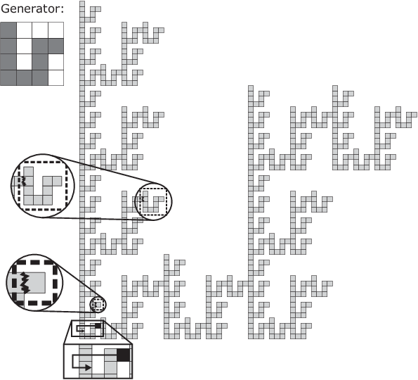
In Figure 3 below, the bottom and top (circular) magnifications show the windows $W_{2}^{1}(0,1,3,2)$ and $W_{3}^{1}(0,1,3,2)$ , respectively.

Next, we will need to translate a small window to a position inside a larger window. These two windows will correspond to squares at the same relative position in different stages $i$ and $j$ of a $g$ -dssf.

Notation.

Let $c\in\mathbb{Z}^{+}$ , $1<i\in\mathbb{N}$ , $1<j\in\mathbb{N}$ , with $i<j$ , and $e,f,xsp,q\in\mathbb{N}_{g}$ . We use $\vec{t}^{c}_{i\rightarrow j}(e,f,p,q)$ to denote the vector joining the southwest corner of $W_{i}^{c}(e,f,p,q)$ to the southwest corner of $W_{j}^{c}(e,f,p,q)$ . In other words, $\vec{t}^{c}_{i\rightarrow j}(e,f,p,q)=\left(c\left(g^{j-1}-g^{i-1}\right)e+c\left(g^{j-2}-g^{i-2}\right)p,c\left(g^{j-1}-g^{i-1}\right)f+c\left(g^{j-2}-g^{i-2}\right)q\right)$ .

For example, in Figure 3 below, $\vec{t}_{2\rightarrow 3}^{1}(0,1,3,2)=(9,18)$ .

To apply Lemma 2.6, we will need the bond-forming submovies to line up. Therefore, once the two square windows share their southwest corner after using the translation defined above, we will need to further translate the smallest one either up or to the right, or both, depending on which side of the windows contains the bond-forming glues, which, in the case of scaled pier fractals, always form a straight (vertical or horizontal) line of length $c$ . We will compute the coordinates of this second translation in our main proof. For now, we establish an upper bound on these coordinates that will ensure that the translated window will remain enclosed in the larger window.

Lemma 3.1.

Let $c\in\mathbb{Z}^{+}$ , $1<i\in\mathbb{N}$ , $1<j\in\mathbb{N}$ , with $i<j$ , $e,f,p,q\in\mathbb{N}_{g}$ , and $x,y\in\mathbb{N}$ . Let $m=c(g^{j-2}-g^{i-2})$ . If $x\leq m$ and $y\leq m$ , then the window $W^{c}_{i}(e,f,p,q)+\vec{t}^{c}_{i\rightarrow j}(e,f,p,q)+(x,y)$ is enclosed in the window $W^{c}_{j}(e,f,p,q)$ .

Proof.

Let $W$ and $w$ denote $W^{c}_{j}(e,f,p,q)$ and $W^{c}_{i}(e,f,p,q)+\vec{t}^{c}_{i\rightarrow j}(e,f,p,q)$ , respectively. Since $W$ and $w$ are square windows that have the same southwest corner and whose respective sizes are $cg^{j-2}$ and $cg^{i-2}$ , $W$ encloses $w$ . The eastern side of $w+(x,0)$ still lies within $W$ , because the maximum value of $x$ is equal to the difference between the size of $W$ and the size of $w$ . The same reasoning applies to a northward translation of $w$ by $(0,y)$ . In conclusion, $w+(x,y)$ must be enclosed in $W$ , as long as neither $x$ nor $y$ exceeds $m$ . ∎

Finally, in our main result, we will use the fact that, for any scaled pier fractal $\mathbf{P}^{c}$ , we can find an infinite number of closed windows that all cut the fractal along a single line of glues (see Lemma 3.5 below), the proof of which uses the following three intermediate lemmas.

Lemma 3.2.

If $\mathbf{P}$ is any pier fractal with generator $G$ , then $G$ contains at least one pier that is not a double-bridge pier.

Proof.

For the sake of obtaining a contradiction, assume that $G$ contains exactly one pier, say $(p,q)$ , and that $(p,q)$ is a double-bridge pier. Note that any double-bridge pier must be positioned at one of the corners of $G$ , that is, $(p,q)\in\{(0,0),(g-1,0),(0,g-1),(g-1,g-1)\}$ . Without loss of generality, assume that $(p,q)=(g-1,0)$ , as in Figure 1 above. Since $(p,q)$ is a double-bridge pier, $(0,0)$ must be the other point in the h-bridge and $(g-1,g-1)$ must be the other point in the v-bridge. Thus, $(0,0)\in G$ (this is also true by definition of $G$ ) and $(g-1,g-1)\in G$ . Since $(p,q)$ is the only pier in $G$ , $(0,0)$ cannot be north-free (nor east-free), which implies that $(0,1)\in G$ . Therefore, $(g-1,1)\not\in G$ (otherwise, $G$ would contain a second h-bridge). Similarly, since $(p,q)$ is the only pier in $G$ , $(g-1,g-1)$ cannot be west-free (nor south-free), which implies that $(g-2,g-1)\in G$ . Therefore, $(g-2,0)\not\in G$ (otherwise, $G$ would contain a second v-bridge). In conclusion, the point $(p,q)=(g-1,0)$ is in $G$ but it is not connected to the rest of $G$ , which contradicts the definition of $\mathbf{P}$ , whose generator must be connected. ∎

Lemma 3.3.

Let $\mathbf{P}$ be any pier fractal with generator $G$ such that $(p,q)\in G$ is a parallel single-bridge pier. If $c\in\mathbb{Z}^{+}$ , then it is always possible to pick one point $(e,f)$ in $G$ such that, for $1<s\in\mathbb{N}$ , $W^{c}_{s}(e,f,p,q)$ encloses a configuration that is connected to $\mathbf{P}^{c}$ via a single connected line of glues of length $c$ .

Proof.

Without loss of generality, assume that the pier $(p,q)$ is pointing north, that it belongs to a v-bridge and that $q=g-1$ (a similar reasoning holds if $q=0$ and the pier points south, or if the pier belongs to an h-bridge and points either west or east). Now, we must pick a point $(e,f)$ such that any window of the form $W^{c}_{s}(e,f,p,q)$ has exactly three free sides. We distinguish two cases.

1.

If $p=0$ , that is, the pier is in the leftmost column of $G$ , then $(1,g-1)\not\in G$ , since $(0,g-1)$ is a north-pointing pier. Therefore, there must exist at least one point in $G\cap(\{1\}\times\mathbb{N}_{g-1})$ , say $(1,y)$ , with $0\leq y<g-1$ , that is north-free. In this case, we pick $(e,f)$ to be equal to $(1,y)$ . Now, consider any window $w$ of the form $W^{c}_{s}(e,f,p,q)$ . The north side of $w$ is free (since $q=g-1$ , $(e,f)$ is north-free in $G$ and $f=y<g-1$ ), the east side of $w$ is free (since $(1,g-1)\not\in G$ ), and the west side of $w$ is free (since the facts that $(0,0)\in G$ , $(0,g-1)\in G$ and $(0,g-1)$ is a single-bridge pier together imply that $(g-1,g-1)\not\in G$ ). Furthermore, since $(0,g-1)$ is a north-pointing pier, $S(0,g-1)\in G$ .
2.

If $p>0$ , then $(p-1,g-1)\not\in G$ . Therefore, there must exist at least one point in $G\cap(\{p-1\}\times\mathbb{N}_{g-1})$ , say $(p-1,y)$ , with $0\leq y<g-1$ , that is north-free. In this case, we pick $(e,f)$ to be equal to $(p-1,y)$ . Now, consider any window $w$ of the form $W^{c}_{s}(e,f,p,q)$ . The north side of $w$ is free (since $q=g-1$ , $(e,f)$ is north-free in $G$ and $f=y<g-1$ ), the west side of $w$ is free (because $(p-1,g-1)\not\in G$ ), and the east side of $w$ is free (since, either $p<g-1$ and $(p+1,g-1)\not\in G$ , or $p=g-1$ , in which case the facts that $(g-1,g-1)\in G$ , $(g-1,0)\in G$ and $(g-1,g-1)$ is a single-bridge pier together imply that $(0,g-1)\not\in G$ ). Furthermore, since $(p,g-1)$ is a north-pointing pier, $S(p,g-1)\in G$ .

Therefore, in both cases, $W^{c}_{s}(e,f,p,q)$ has exactly three free sides and encloses a configuration that is connected to $\mathbf{P}^{c}$ via a single connected horizontal line of glues of length $c$ positioned on the south side of the window.

∎

Lemma 3.4.

Let $\mathbf{P}$ be any pier fractal with generator $G$ such that $(p,q)\in G$ is an orthogonal single-bridge pier. If $c\in\mathbb{Z}^{+}$ , then it is always possible to pick one point $(e,f)$ in $G$ such that, for $1<s\in\mathbb{N}$ , $W^{c}_{s}(e,f,p,q)$ encloses a configuration that is connected to $\mathbf{P}^{c}$ via a single connected line of glues of length $c$ .

Proof.

Without loss of generality, assume that the pier $(p,q)$ is pointing east, that it belongs to a v-bridge and that $q=g-1$ (a similar reasoning holds if $q=0$ , or if the pier points west, or if the pier belongs to an h-bridge and points either north or south). Note that, in this case, $g$ must be strictly greater than 2, since $(p,g-1)\in G$ , $(p,0)\in G$ but $(p,g-2)\not\in G$ . Now, we must pick a point $(e,f)$ such that any window of the form $W^{c}_{s}(e,f,p,q)$ has exactly three free sides. We distinguish two cases.

1.

If $p<g-1$ , then $(p,g-2)\not\in G$ , since $(p,g-1)$ is an east-pointing pier. Therefore, there must exist at least one point in $G\cap(\{p\}\times\mathbb{N}_{g-2})$ , say $(p,y)$ , with $0\leq y<g-2$ , that is north-free. In this case, we pick $(e,f)$ to be equal to $(p,y)$ . Now, consider any window $w$ of the form $W^{c}_{s}(e,f,p,q)$ . The north side of $w$ is free (since $q=g-1$ , $(e,f)$ is north-free in $G$ and $f=y<g-2<g-1$ ), the east side of $w$ is free (since $p<g-1$ and $(p+1,g-1)\not\in G$ ), and the south side of $w$ is free (since $(p,g-2)\not\in G$ ). Furthermore, since $(p,g-1)$ is an east-pointing pier, $W(p,g-1)\in G$ .
2.

If $p=g-1$ , that is, the pier is in the rightmost column of $G$ , then the facts that $(g-1,0)\in G$ , $(g-1,g-1)\in G$ and $(g-1,g-1)$ is a single-bridge pier together imply that $(0,g-1)\not\in G$ . This, together with the fact that $(0,0)\in G$ , implies that there must exist at least one point in $G\cap(\{0\}\times\mathbb{N}_{g-1})$ , say $(0,y)$ , with $0\leq y<g-1$ , that is north-free. In this case, we pick $(e,f)$ to be equal to $(0,y)$ . Now, consider any window $w$ of the form $W^{c}_{s}(e,f,p,q)$ . The north side of $w$ is free (since $q=g-1$ , $(e,f)$ is north-free in $G$ and $f=y<g-1$ ), the east side of $w$ is free (since $(0,g-1)\not\in G$ ), and the south side of $w$ is free (since $(p,g-2)\not\in G$ ). Furthermore, since $(g-1,g-1)$ is an east-pointing pier, $W(g-1,g-1)\in G$ .

∎

Lemma 3.5.

Let $\mathbf{P}$ be any pier fractal with generator $G$ . If $c\in\mathbb{Z}^{+}$ , then it is always possible to pick one pier $(p,q)$ and one point $(e,f)$ , both in $G$ , such that, for $1<s\in\mathbb{N}$ , $W^{c}_{s}(e,f,p,q)$ encloses a configuration that is connected to $\mathbf{P}^{c}$ via a single connected (horizontal or vertical) line of glues of length $c$ .

Proof.

Let $\mathbf{P}$ be any pier fractal with generator $G$ . Let $c\in\mathbb{Z}^{+}$ and $1<s\in\mathbb{N}$ . By definition of a pier fractal, $G$ contains at least one pier. We will pick one of these piers carefully.

According to Lemma 3.2, it is always possible to choose a pier in $G$ that is not a double-bridge pier. Therefore, we can always choose either a real pier or a single-bridge pier. We now consider the three possible cases.

First, if $G$ contains one or more real piers, we can simply choose one of them as $(p,q)$ . In this case, we pick $(e,f)=(p,q)$ , since any window of the form $W^{c}_{s}(p,q,p,q)$ , where $(p,q)$ is a real pier in $G$ , must have exactly three free sides. Therefore, $W^{c}_{s}(p,q,p,q)$ must enclose a configuration that is connected to $\mathbf{P}^{c}$ via a single line of glues of length $c$ , namely on its non-free side.

Second, if $G$ does not contain any real piers, $G$ must contain at least one single-bridge pier. So we wrap up this proof by considering the two types of single-bridge piers.

If $G$ contains at least one parallel single-bridge pier, according to Lemma 3.3, it is always possible to choose one pier $(p,q)$ and one point $(e,f)$ , both in $G$ , such that, for $1<s\in\mathbb{N}$ , $W^{c}_{s}(e,f,p,q)$ encloses a configuration that is connected to $\mathbf{P}^{c}$ via a single connected line of glues of length $c$ .

Finally, if $G$ contains at least one orthogonal single-bridge pier, according to Lemma 3.4, it is always possible to choose one pier $(p,q)$ and one point $(e,f)$ , both in $G$ , such that, for $1<s\in\mathbb{N}$ , $W^{c}_{s}(e,f,p,q)$ encloses a configuration that is connected to $\mathbf{P}^{c}$ via a single connected line of glues of length $c$ . ∎

3.2 Main result

We are now ready to prove our main result.

Theorem 3.6.

Let $\mathbf{P}$ be any pier fractal. If $c\in\mathbb{Z}^{+}$ , then $\mathbf{P}^{c}$ does not strictly self-assemble in the aTAM.

Proof.

Let $\mathbf{P}$ be any pier fractal with a $g\times g$ generator $G$ , where $1<g\in\mathbb{N}$ . Let $c$ be any positive integer. For the sake of obtaining a contradiction, assume that $\mathbf{P}^{c}$ does strictly self-assemble in some TAS $\mathcal{T}=(T,\sigma,\tau)$ . Further assume that $\vec{\alpha}$ is some assembly sequence in $\mathcal{T}$ whose result is $\alpha$ , such that ${\rm dom}\;\alpha=\mathbf{P}^{c}$ .

	Translation Formulas for $(x,y)$
North-pointing Pier Vertical Bridge with Southern Bridge Point at $(a,0)$		$x=ac\Sigma_{k=i-2}^{j-3}g^{k}$ $y=0$
East-pointing Pier Horizontal Bridge with Western Bridge Point at $(0,b)$		$x=0$ $y=bc\Sigma_{k=i-2}^{j-3}g^{k}$
South-pointing Pier Vertical Bridge with Northern Bridge Point at $(a,g-1)$		$x=ac\Sigma_{k=i-2}^{j-3}g^{k}$ $y=c(g^{j-2}-g^{i-2})$
West-pointing Pier Horizontal Bridge with Eastern Bridge Point at $(g-1,b)$		$x=c(g^{j-2}-g^{i-2})$ $y=bc\Sigma_{k=i-2}^{j-3}g^{k}$

According to Lemma 3.5, we can always pick one pier $(p,q)$ and a point $(e,f)$ , both in $G$ , such that, for $1<s\in\mathbb{N}$ , the window $W^{c}_{s}(e,f,p,q)$ , which we will abbreviate $w_{s}$ , encloses a configuration that is connected to $\mathbf{P}^{c}$ via a single line of glues of length $c$ .³³ 3 Without loss of generality, we will assume that this line of glues is positioned on the western side of the windows and is thus vertical (see the jagged lines in Figure 3, where $s=2$ and $s=3$ for the small and large windows, respectively, and $(p,q)=(3,2)$ and $(e,f)=(0,1)$ ), because the chosen pier in our example points east. A similar reasoning holds for piers pointing north, south or west. The maximum number of distinct combinations and orderings of glue positionings along this line of glues is finite.⁴⁴ 4 This number is bounded above by $T_{glue}^{2c}\cdot(2c)!$ , where $T_{glue}$ is the total number of distinct glue types in $T$ . By the generalized pigeonhole principle, since $\left|\left\{w_{s}~\left|~1<s\in\mathbb{N}\right.\right\}\right|$ is infinite, there must be at least one bond-forming submovie such that an infinite number of windows generate this submovie (up to translation). Let us pick two such windows, say, $w_{i}$ and $w_{j}$ with $i<j$ , such that $\mathcal{B}(M_{\vec{\alpha},w_{i}})$ and $\mathcal{B}(M_{\vec{\alpha},w_{j}})$ are equal (up to translation). We must pick these windows carefully, since as stated in the proof of Lemma 2.6, the seed of $\alpha$ must be either in both windows or in neither. This condition can always be satisfied. The only case where the seed is in more than one window is when it is at position $(0,0)$ and $e=f=p=q=0$ , which implies that all windows include the origin. So, in this case, any choice of $i$ and $j>i$ will do. In all other cases, none of the windows overlap. So, if the seed belongs to one of them, say $w_{k}$ , then we can pick any $i$ greater than $k$ (and $j>i$ ). Finally, if the seed does not belong to any windows, then any choice of $i$ and $j>i$ will do.

We will now prove that $w_{i}$ and $w_{j}$ satisfy the two conditions of Lemma 2.6.

First, we compute $\vec{c}$ such that $\mathcal{B}(M_{\vec{\alpha},w_{i}})+\vec{c}=\mathcal{B}(M_{\vec{\alpha},w_{j}})$ . We know that $w_{i}+\vec{t}^{c}_{i\rightarrow j}(e,f,p,q)$ and $w_{j}$ share their southwest corner. We need to perform one more translation $(x,y)$ to align the bond-forming glues of $w_{i}$ and $w_{j}$ . The values of $x$ and $y$ depend on the direction in which the chosen pier is pointing. The formulas corresponding to all four directions are given in Figure 4. Furthermore, a justification for the recurring summation in the formulas of Figure 4 is provided in Figure 5. In that figure, the chosen case is a north-pointing pier. However, our example in Figure 3 above uses an east-pointing pier. We now complete the proof for this case. To align the bond-forming glues of $w_{i}$ and $w_{j}$ , we must translate $w_{i}+\vec{t}^{c}_{i\rightarrow j}(e,f,p,q)$ by $(x,y)=\left(0,bc\sum_{k=i-2}^{j-3}g^{k}\right)$ , with $b\leq g-1$ . Since $x=0\leq m$ (as defined in Lemma 3.1) and $y=bc\sum_{k=i-2}^{j-3}g^{k}\leq(g-1)c\sum_{k=i-2}^{j-3}g^{k}=c\left(\sum_{k=i-1}^{j-2}g^{k}-\sum_{k=i-2}^{j-3}g^{k}\right)=c\left(g^{j-2}-g^{i-2}\right)=m$ , we can apply Lemma 3.1 to infer that, with $\vec{c}=\vec{t}^{c}_{i\rightarrow j}(e,f,p,q)+(x,y)$ , $w_{i}+\vec{c}$ is enclosed in $w_{j}$ . Therefore, the second condition of Lemma 2.6 holds.

Second, by construction, $\mathcal{B}(M_{\vec{\alpha},w_{i}})+\vec{c}=\mathcal{B}(M_{\vec{\alpha},w_{j}})$ . Therefore, the first condition of Lemma 2.6 holds.

In conclusion, the two conditions of Lemma 2.6 are satisfied, with $\alpha_{I}$ and $\alpha_{O}^{\prime}$ defined as the intersection of $\mathbf{P}^{c}$ with the inside of $w_{i}$ and the outside of $w_{j}$ , respectively. We can thus conclude that the assembly $\alpha_{O}^{\prime}\cup(\alpha_{I}+\vec{c})$ is producible in $\mathcal{T}$ . Note that this assembly is identical (up to translation) to $\mathbf{P}^{c}$ , except that the interior of the large window $w_{j}$ is replaced by the interior of the small window $w_{i}$ . Since the configurations in these two windows cannot be identical, we have proved that $\mathcal{T}$ does not strictly self-assemble $\mathbf{P}^{c}$ , which is a contradiction.

∎

3.3 Corollaries of our main result

In this section, we discuss both special cases and generalizations of our main result.

3.3.1 Specializations of our main result

In [1], we proved that no scaled tree fractal strictly self-assembles in the aTAM, where a tree fractal is a discrete self-similar fractal whose underlying graph is a tree. In this section, we start by proving a new characterization of tree fractals in terms of simple connectivity properties of their generator.

Theorem 3.7.

$\displaystyle\mathbf{T}=\bigcup_{i=1}^{\infty}{T_{i}}$ is a $g$ -discrete self-similar tree fractal, for some $g>1$ , with generator $G$ if and only if
a. $G$ is a tree and
b. $nhb_{G}=nvb_{G}=1.$

The proof of this theorem is in the appendix. Next, the following observation follows from the fact that a tree with more than one vertex must contain at least two leaf nodes.

Observation 3.8.

If $G$ is the generator of any discrete self-similar fractal and $G$ is a tree, then it must contain at least two piers.

Finally, we can recast the main result in [1] as a special case of our main result.

Corollary 3.9.

[From [1]] Let $\mathbf{T}$ be any tree fractal. If $c\in\mathbb{Z}^{+}$ , then $\mathbf{T}^{c}$ does not strictly self-assemble in the aTAM.

Proof.

Let $\mathbf{T}$ be any tree fractal with generator $G$ . According to Theorem 3.7, the full grid graph of $G$ is a tree and is thus connected, and $nhb_{G}=nvb_{G}=1$ . Furthermore, according to Observation 3.8, $G$ must contain at least one pier. Therefore, $\mathbf{T}$ is a pier fractal and $\mathbf{T}^{c}$ does not strictly self-assemble in the aTAM. ∎

We now turn our attention to a second specialization of our main result by considering “pinch-point fractals,” which are defined in [6] as follows.

Definition 3.10.

Let $\mathbf{X}\subset\mathbb{N}^{2}$ be a $g$ -discrete self-similar fractal with generator $G$ . We say that $\mathbf{X}$ is a pinch-point discrete self-similar fractal if $G$ satisfies the following four conditions:

1.

$\{(0,0),(0,g-1),(g-1,0)\}\subseteq G$ .
2.

$G\cap(\{1,\ldots,g-1\}\times\{g-1\})=\varnothing$ .
3.

$G\cap(\{g-1\}\times\{1,\ldots,g-1\})=\varnothing$ .
4.

The full grid graph of $G$ is connected.

Theorem 3.12 in [6] establishes that no pinch-point fractal strictly self-assembles in the aTAM. We can now generalize this result as follows.

Corollary 3.11.

Let $\mathbf{X}$ be any pinch-point discrete self-similar fractal. If $c\in\mathbb{Z}^{+}$ , then $\mathbf{X}^{c}$ does not strictly self-assemble in the aTAM.

Proof.

Let $\mathbf{X}$ be any pinch-point discrete self-similar fractal with generator $G\subset\mathbb{N}_{g}^{2}$ , for some $g>1$ . First, by definition of a pinch-point fractal, the full grid graph of $G$ is connected. Second, since the point $(g-1,0)$ is the only point of $G$ that belongs to $\{g-1\}\times\mathbb{N}$ and the point $(0,0)$ also belongs to $G$ , $nhb_{G}=1$ . Similarly, since the point $(0,g-1)$ is the only point of $G$ that belongs to $\mathbb{N}\times\{g-1\}$ and the point $(0,0)$ also belongs to $G$ , $nvb_{G}=1$ . Third, since the point $(0,g-1)$ is a pier in $G$ , $G$ contains at least one pier. Therefore, $\mathbf{X}$ is a pier fractal. In conclusion, if $c\in\mathbb{Z}^{+}$ , then $\mathbf{X}^{c}$ does not strictly self-assemble in the aTAM.

∎

3.3.2 Generalizations of our main result

We now discuss how to extend our main result to different classes of fractals. More specifically, we will relax the last two conditions in the definition of pier fractals and still be able to use the same reasoning as we did in the proof of our main result.

First, our proof of Theorem 3.6 uses the fact that there exist an infinite collection of square windows, each of which encloses a sub-configuration of the fractal that is attached to the rest of the fractal at a single point (or single line of points). In other words, each window in the collection has three free sides. If, for example, the east and west sides of each window are free, then the number of horizontal bridges in the generator $G$ does not matter. Even if $nhb_{G}>1$ , our construction for the windows still works. Figure 6 is one example of such a fractal to which our main result generalizes, with the first three windows shown as thick, black squares. In this case, our proof technique still works, even though the generator contains three horizontal bridges. Here is a precise statement of the corollary.

Corollary 3.12.

Let $\mathbf{F}$ be a discrete self-similar fractal with generator $G$ such that the full grid graph of $G$ is connected, $nvb_{G}=1$ , and $G$ contains at least one north-pointing pier or one south-pointing pier. If $c\in\mathbb{Z}^{+}$ , then $\mathbf{F}^{c}$ does not strictly self-assemble in the aTAM.

Symmetrically, a similar result holds for fractals whose generator $G$ contains either at least one west-pointing pier or at least one east-pointing pier, and such that $nhb_{G}=1$ .

Second, having relaxed the second condition (part $b$ ) of the definition of pier fractals, we can now relax the third condition (part $c$ ) as well. To apply our Closed Window Movie Lemma, a pier is not strictly needed. Instead, the generator only need contain a pier-like sub-configuration, that is, a sub-configuration of one or more tiles that is attached to the rest of the fractal at a single point. Figure 7 gives one example of such a fractal with the first two windows shown as thick, solid, black squares. In this case, our proof technique still works, even though the generator contains five horizontal bridges and no pier. Here is a precise statement of the corollary.

Corollary 3.13.

Let $\mathbf{F}$ be a discrete self-similar fractal with generator $G$ such that the full grid graph of $G$ is connected, $nvb_{G}=1$ , and $G$ contains at least one north-pointing pier-like sub-configuration or at least one south-pointing pier-like sub-configuration. If $c\in\mathbb{Z}^{+}$ , then $\mathbf{F}^{c}$ does not strictly self-assemble in the aTAM.

Symmetrically, a similar result holds for fractals whose generator $G$ contains either at least one west-pointing pier-like sub-configuration or at least one east-pointing pier-like sub-configuration, and such that $nhb_{G}=1$ .

Finally, the Closed Window Movie Lemma may be applicable even when the generator does not contain any pier-like sub-configuration. The key requirement in the proof of our main result is to be able to find at least two windows that share a common bond-forming window movie but whose insides contain different sub-configurations. This requirement can be met even when the sub-configuration contained in each window is attached to the rest of the fractal at more than one point. Figure 8 illustrates such a situation. For a general characterization, we need some definitions.

If $G$ is a $g\times g$ generator, then a column is any set $G\cap(\{x\}\times\mathbb{N}_{g}$ ), where $x\in\mathbb{N}_{g}$ is the index of the column. Therefore, columns are indexed from left to right starting at 0. Two columns are equivalent if they contain the same number of points and, for each point in one column, there is a point in the other column with the same $y$ coordinate. A vertical cut is any set of edges connecting two adjacent columns of $G$ . Two vertical cuts are equivalent if they contain the same number of edges and, for each edge in one cut, there is an edge in the other cut with the same $y$ coordinate. Figure 8 depicts a $5\times 5$ generator $G$ in which columns 2 and 3 are equivalent. Furthermore, in this example, cuts 2 and 3 are also equivalent.⁵⁵ 5 The index of a vertical cut is given by the index of the leftmost of the two columns that its edges connect. Note that the fact that two columns $i$ and $j$ are equivalent does not imply that the vertical cuts $i$ and $j$ are also equivalent. That both facts hold is just a coincidence in this example. If, for example, the point $(4,1)$ were removed from the generator in Figure 8, then columns 2 and 3 would still be equivalent, but vertical cuts 2 and 3 would no longer be equivalent.⁶⁶ 6 We included point $(4,1)$ in the generator to exclude piers from the generator in this example. In general, there is no correlation between the indices of equivalent columns and the indices of equivalent vertical cuts. However, the co-existence of equivalent columns and equivalent vertical cuts in the same generator may render the Window Movie Lemma applicable.

In the example of Figure 8, vertical cut 2 is to the east of the vertical bridge (which is a subset of column 1). Therefore, if we can find an east-free point in $G$ , e.g., the point $(1,0)$ in our running example, we will be able to position a closed window that only cuts the fractal on one side (here, its western side), e.g., the smallest of the two solid windows in Figure 8. Similarly, we can position another closed window of the same size that cuts the generator through vertical cut 3, e.g., the dotted window that overlaps the small solid window. By construction, the window movies corresponding to these two windows have the same length and contain exactly the same positions (up to translation). Of course, these window movies may not be equal up to translation because the glues in their respective positions may not match. But this is where we can take advantage of the existence of two equivalent columns. By self-similarity, these two columns will, in the next stage of the fractal, become two 5-wide sets of columns of height 20 that are pairwise equivalent, that is, columns $c_{1}$ and $c^{\prime}_{1}$ are equivalent, columns $c_{2}$ and $c^{\prime}_{2}$ are equivalent, …, and columns $c_{5}$ and $c^{\prime}_{5}$ are equivalent. More importantly, the 20-high cuts labeled a, b, c, and d in Figure 8 are all pairwise equivalent. Therefore, at this stage of the fractal, we can build four larger square windows, as shown in Figure 8. Furthermore, at each successive stage of the fractal, we will be able to build twicef⁷⁷ 7 Note that, in this example, cut 1 is also equivalent to cuts 2 and 3. So we can actually build three windows for each one of the equivalent columns in the generator. Therefore, we could could have drawn 3, 6, 12, etc. windows for stages 2, 3, 4, etc., respectively. However, we chose to use only two of the three equivalent cuts in our discussion in order to keep the figure as legible as possible. as many square windows that all generate window movies of the same length and with positions that are equal up to translation. Since the number of window movies grows without bound as the stage number increases, but the number of distinct combinations and orderings of glue positionings is finite (following a reasoning similar to the one in Footnote 4), there is always a stage (in fact, an infinite number of them) that contains two bond-forming window movies that are identical up to translation. The sub-configurations inside the two corresponding windows cannot be equivalent because of the way the windows overlap. Additionally, since the two windows have exactly the same shape and size, the translation of the eastmost one is enclosed in (in fact, equal to) the other one. Therefore, we can apply the Closed Window Movie Lemma and conclude the proof by contradiction. Here is a precise statement of the corollary that covers the class of similar situations.

Corollary 3.14.

Let $\mathbf{F}$ be a discrete self-similar fractal with generator $G$ such that the full grid graph of $G$ is connected, $G$ contains two equivalent columns, and $G$ contains two equivalent vertical cuts that are positioned on the same side of all vertical bridges. If $c\in\mathbb{Z}^{+}$ , then $\mathbf{F}^{c}$ does not strictly self-assemble in the aTAM.

Symmetrically, a similar result holds for fractals with equivalent rows and equivalent horizontal cuts.

To conclude this section, we note that Corollary 3.14 could have been proved using the standard Window Movie Lemma introduced in [5], since the windows used in the proof have exactly the same shape and size. In the next section, we motivate our introduction of the Closed Window Movie Lemma as a more convenient tool in the study of scaled pier fractals.

4 Discussion

A fair question for one to ask is: why not simply prove Theorem 3.6 using the standard Window Movie Lemma from [5]? Our response is that we currently do not know that we cannot.

For the sake of discussion, the statement of the standard WML, restricted to bond-forming submovies, is as follows.

Lemma 4.1 (Standard Window Movie Lemma [5]).

Let $\vec{\alpha}~=~(\alpha_{i}~|~0\leq~i<~l)$ and $\vec{\beta}~=~(\beta_{i}~|~0\leq~i<~m)$ , with $l,m\in\mathbb{Z}^{+}\cup\{\infty\}$ , be assembly sequences in some TAS $\mathcal{T}$ with results $\alpha$ and $\beta$ , respectively. Let $w$ be a window that partitions $\alpha$ into two configurations $\alpha_{L}$ and $\alpha_{R}$ , and, for some $\vec{c}\neq(0,0)$ , $w^{\prime}=w+\vec{c}$ be a translation of $w$ that partitions $\beta$ into two configurations $\beta_{L}$ and $\beta_{R}$ . Furthermore, define $M_{\vec{\alpha},w}$ and $M_{\vec{\beta},w^{\prime}}$ to be the respective window movies for $\vec{\alpha},w$ and $\vec{\beta},w^{\prime}$ and define $\alpha_{L},\beta_{L}$ to be the sub-configurations of $\alpha$ and $\beta$ containing the seed tiles of $\alpha$ and $\beta$ , respectively. Then, if $\mathcal{B}\left(M_{\vec{\alpha},w}\right)+\vec{c}=\mathcal{B}\left(M_{\vec{\beta},w^{\prime}}\right)$ , it is the case that the following two assemblies are also producible: (1) the assembly $\alpha_{L}\beta^{\prime}_{R}=\alpha_{L}\cup\beta^{\prime}_{R}$ and (2) the assembly $\beta^{\prime}_{L}\alpha_{R}=\beta^{\prime}_{L}\cup\alpha_{R}$ , where $\beta^{\prime}_{L}=\beta_{L}-\vec{c}$ and $\beta^{\prime}_{R}=\beta_{R}-\vec{c}$ .

Basically, the reason we do not use the standard WML to prove Theorem 3.6 is because we simply are not able to devise a unified strategy for finding two closed-rectangular window movies in a pier-fractal-shaped assembly that (1) have equivalent (up to translation) bond-forming submovies and (2) contain different sub-shapes of the assembly. On the one hand, it is trivial to find two such closed-rectangular window movies in a pier-fractal-shaped assembly whose sub-shapes are equal. But this does not help us derive the contradiction that we need to prove Theorem 3.6. On the other hand, it is also trivial to find two closed-rectangular window movies that contain different sub-shapes of the assembly, but, as a result of the self-similarity of pier fractals, do not have equivalent (up to translation) bond-forming submovies, at which point the conditions of the hypothesis of the standard WML are no longer satisfied.

In our attempts to resolve this dilemma, we investigated the use of an infinite-open window strategy, as opposed to a closed-rectangular window strategy. But this approach has its own set of technical challenges. Fortunately, these challenges can be dismissed! One must simply observe that, in order to prove Theorem 3.6, one does not need the “two-way-assembly-replacement” power offered by the conclusion of the standard WML. In fact, in order to derive a contradiction to prove Theorem 3.6, one merely needs to be able to replace one portion of a tile assembly with another portion in a strictly “one-way” fashion, i.e., the part of the tile assembly being used to replace another part does not need to be able to be replaced by the part of the tile assembly it is replacing. Thus, we weaken the conclusion and strengthen the hypothesis of the standard WML to get the Closed WML, which turns out to be much more accommodating to a unified, closed-rectangular window proof technique for pier fractals.

It appears that the hypothesis of the standard WML, unlike that of the Closed WML, is too strong to be able to “handle” all pier fractals under a unified closed-rectangular window proof technique. However, it is worthy of note that in some special cases, it is possible to use the standard WML to prove that certain pier fractals do not strictly self-assemble. For example, it is possible to prove that the Sierpinski triangle does not strictly self-assemble at any positive scale factor (see Figure 9 for the proof idea). Next, consider the tree fractal defined by the generator given in Figure 10. In this case, it is possible to apply the standard WML using an open-infinite window proof technique (informally depicted in Figure 10). Unfortunately, depending on the geometry of the particular fractal, neither of the previous two applications of the standard WML, either with closed-rectangular or open-infinite windows, immediately generalizes to even the set of all tree fractals, which is a strict sub-class of pier fractals. Even more troubling, we suspect that, for the pier fractal whose generator is shown in Figure 11, it is not possible to apply the standard WML, with windows of any shape, to prove that it does not strictly self-assemble at any positive scale factor.

Figure 11: How can one apply the standard WML to prove that any scaled version of the pier fractal with this generator does not strictly self-assemble?

5 Conclusion

In this paper, we made three contributions. First, we gave a new characterization of tree fractals in terms of simple geometric properties of their generator (see Section 6). Second, we proved a new variant of the Window Movie Lemma in [5], which we call the “Closed Window Movie Lemma” (see Section 2.3). Third, we proved that no scaled-up version of any discrete self-similar pier fractal strictly self-assembles in the aTAM (see Section 3.2).

As we pointed out in Section 3.3.2, the scope of applicability of the Closed Window Movie Lemma is much wider than the class of pier fractals. Recall that Corollary 3.14 applies the Closed Window Movie Lemma to discrete self-similar fractals with no pier-like sub-configurations and an arbitrary number of vertical and horizontal bridges. In future work, we would like to provide a characterization of the class of all fractals to which the Closed Window Movie Lemma applies, that is, a strict super-class of the class of pier fractals. In addition, it would be satisfying to find a crisp characterization of the differences (if any) between the scope of applicability of the standard WML and that of the Closed WML. For instance, we would like to prove our conjecture that it is not possible to use the standard WML to prove that any scaled version of the pier fractal whose generator is shown in Figure 11 does not strictly self-assemble in the aTAM.

Acknowledgments

We would like to thank Kimberly Barth and Paul Totzke for contributing to an earlier proof of Corollary 3.9 that appeared in [1] and that we generalized to obtain the proof of our main result in this work.

References

[1] Kimberly Barth, David Furcy, Scott M. Summers, and Paul Totzke, Scaled tree fractals do not strictly self-assemble, Proceedings of the 13th International Conference on Unconventional Computation and Natural Computation (UCNC 2014), to appear.
[2] David Doty, Xiaoyang Gu, Jack H. Lutz, Elvira Mayordomo, and Philippe Moser, Zeta-Dimension, Proceedings of the Thirtieth International Symposium on Mathematical Foundations of Computer Science, Springer-Verlag, 2005, pp. 283–294.
[3] James I. Lathrop, Jack H. Lutz, and Scott M. Summers, Strict self-assembly of discrete Sierpinski triangles, Theoretical Computer Science 410 (2009), 384–405.
[4] Jack H. Lutz and Brad Shutters, Approximate self-assembly of the sierpinski triangle, Theory Comput. Syst. 51 (2012), no. 3, 372–400.
[5] P.-E. Meunier, M. J. Patitz, S. M. Summers, G. Theyssier, A. Winslow, and D. Woods, Intrinsic universality in tile self-assembly requires cooperation, Proceedings of the 25th Annual ACM-SIAM Symposium on Discrete Algorithms (SODA 2014), 2014, pp. 752–771.
[6] Matthew J. Patitz and Scott M. Summers, Self-assembly of discrete self-similar fractals, Natural Computing 1 (2010), 135–172.
[7] Paul W. K. Rothemund, Theory and experiments in algorithmic self-assembly, Ph.D. thesis, University of Southern California, December 2001.
[8] Nadrian C. Seeman, Nucleic-acid junctions and lattices, Journal of Theoretical Biology 99 (1982), 237–247.
[9] , De novo design of sequences for nucleic acid structural engineering, Journal of Biomolecular Structural Dynamics 8 (1990), 573–581.
[10] Hao Wang, Proving theorems by pattern recognition – II, The Bell System Technical Journal XL (1961), no. 1, 1–41.
[11] Erik Winfree, Algorithmic self-assembly of DNA, Ph.D. thesis, California Institute of Technology, June 1998.

6 Appendix

Definition 6.1.

If $G$ is the generator of any $g$ -discrete self-similar fractal, then the interior of $G$ is $G\cap(\mathbb{N}_{g-1}\times\mathbb{N}_{g-1})$ .

Lemma 6.2.

Let $G$ be any finite subset of $\mathbb{N}^{2}$ that has at least one connected h-bridge. If $G$ contains a connected component $C\subset G$ such that $C\cap(\mathbb{N}\times\{t_{G}\})\neq\varnothing$ and $C\cap(\{l_{G}\}\times\mathbb{N})=\varnothing$ , then there exists a point $\vec{x}_{N}\in G\backslash C$ such that $N\left(\vec{x}_{N}\right)\not\in G$ and $\vec{x}_{N}\not\in\mathbb{N}\times\{t_{G}\}$ .

Proof.

Let $h$ be a connected h-bridge in $G$ and let $\pi$ be a connected component in $G$ that contains a path connecting the two points in $h$ . Since $\pi$ connects the leftmost and rightmost columns of $G$ and $C$ does not contain any point in the leftmost column of $G$ , $C\cap\pi=\varnothing$ . Since $C$ is a connected component that extends vertically from row $t_{C}=t_{G}$ down to row $b_{C}$ and $C\cap\pi=\varnothing$ , $\pi$ must go around (and below) $C$ . Furthermore, no point in $C$ is adjacent to any point in $\pi$ . Let $\vec{p}$ denote a bottommost point $(x,b_{C})$ in $C$ , with $l_{G}<x\leq r_{G}$ . Let $\vec{q}$ denote the topmost point $(x,y)$ in $\pi\cap(\{x\}\times\mathbb{N}_{b_{C}})$ . Note that $\vec{p}$ and $\vec{q}$ are in the same column and that $\vec{p}$ is above (but not adjacent to) $\vec{q}$ , that is, $y<b_{C}-1$ . Furthermore, $N(\vec{q})\notin G$ . Since $\vec{q}\in\pi\subset G$ and $\vec{q}\not\in C$ , $\vec{q}\in G\backslash C$ . Furthermore, since $\vec{q}=(x,y)$ and $y<b_{C}-1<b_{C}\leq t_{C}=t_{G}$ , $\vec{q}\not\in\mathbb{N}\times\{t_{G}\}$ . In conclusion, $\vec{q}$ exists and is a candidate for the role of $x_{N}$ . ∎

Lemma 6.3.

Let $G$ be any finite subset of $\mathbb{N}^{2}$ that has at least one connected v-bridge. If $G$ contains a connected component $C\subset G$ such that $C\cap(\{r_{G}\}\times\mathbb{N})\neq\varnothing$ , $C\cap(\mathbb{N}\times\{t_{G}\})\neq\varnothing$ and $C\cap(\mathbb{N}\times\{b_{G}\})=\varnothing$ , then there exists a point $\vec{x}_{NE}\in G\backslash C$ such that $E\left(\vec{x}_{NE}\right)\not\in G$ , $\vec{x}_{NE}\in\mathbb{N}\times\{t_{G}\}$ and $\vec{x}_{NE}\not\in\{r_{G}\}\times\mathbb{N}$ .

Proof.

Let $v$ be a connected v-bridge in $G$ and let $\pi$ be a connected component in $G$ that contains a path connecting the two points in $v$ . Let $\pi_{t}$ denote the set $\pi\cap(\mathbb{N}\times\{t_{G}\})$ . Since this set cannot be empty, let us call its rightmost point $\vec{p}=(x_{\pi},t_{G})$ . Similarly, let $C_{t}$ denote $C\cap(\mathbb{N}\times\{t_{G}\})$ . Since this set cannot be empty, let us call its leftmost point $\vec{q}=(x_{C},t_{G})$ .

Since $\pi$ connects the topmost and bottommost rows of $G$ and $C$ does not contain any point in the bottommost row of $G$ , $C\cap\pi=\varnothing$ . This, together with the fact that $C$ contains a path from the topmost row to the rightmost column of $G$ (that is, $C$ “cuts off” the subset of $G$ that lies to the north-east of $C$ from the rest of $G$ ), implies that each point in $\pi_{t}$ must appear to the left of all the points in $C_{t}$ , namely $x_{\pi}<x_{C}$ . In fact, since $\pi$ and $C$ cannot be connected, $\vec{p}$ and $\vec{q}$ cannot be adjacent, i.e., $x_{\pi}<x_{C}-1$ . Therefore, $\vec{p}$ and $\vec{q}$ are both in the topmost row of $G$ (thus $\vec{p}\in\mathbb{N}\times\{t_{G}\}$ ) and $\vec{p}$ is to the left of $\vec{q}$ (thus $\vec{p}\not\in\{r_{G}\}\times\mathbb{N}$ ). Finally, by construction, $\vec{p}\in G\backslash C$ and $E(\vec{p})\not\in G$ . In conclusion, $\vec{p}$ is a candidate for the role of $\vec{x}_{NE}$ . ∎

Lemma 6.4.

Let $G$ be any finite subset of $\mathbb{N}^{2}$ that has at least one connected v-bridge. If $G$ contains a connected component $C\subset G$ such that $C\cap(\{r_{G}\}\times\mathbb{N})\neq\varnothing$ and $C\cap(\mathbb{N}\times\{b_{G}\})=\varnothing$ , then there exists a point $\vec{x}_{E}\in G\backslash C$ such that $E\left(\vec{x}_{E}\right)\not\in G$ and $\vec{x}_{E}\not\in\{r_{G}\}\times\mathbb{N}$ .

Proof.

Let $v$ be a connected v-bridge in $G$ and let $\pi$ be a connected component in $G$ that contains a path connecting the two points in $v$ . Since $\pi$ connects the topmost and bottommost rows of $G$ and $C$ does not contain any point in the bottommost row of $G$ , $C\cap\pi=\varnothing$ . Since $C$ is a connected component that extends horizontally from column $l_{C}$ to column $r_{C}=r_{G}$ and $C\cap\pi=\varnothing$ , $\pi$ must go around (and to the left of) $C$ . Furthermore, no point in $C$ is adjacent to any point in $\pi$ . Let $\vec{p}$ denote a leftmost point $(l_{C},y)$ in $C$ , with $b_{G}<y\leq t_{G}$ . Let $\vec{q}$ denote the rightmost point $(x,y)$ in $\pi\cap(\mathbb{N}_{l_{C}}\times\{y\})$ . Note that $\vec{p}$ and $\vec{q}$ are in the same row and that $\vec{q}$ is to the left of (but not adjacent to) $\vec{p}$ , that is, $x<l_{C}-1$ . Furthermore, $E(\vec{q})\notin G$ . Since $\vec{q}\in\pi\subset G$ and $\vec{q}\not\in C$ , $\vec{q}\in G\backslash C$ . Furthermore, since $\vec{q}=(x,y)$ and $x<l_{C}-1<l_{C}\leq r_{C}=r_{G}$ , $\vec{q}\not\in\{r_{G}\}\times\mathbb{N}$ . In conclusion, $\vec{q}$ exists and is a candidate for the role of $x_{E}$ . ∎

Lemma 6.5.

Let $\mathbf{X}=\bigcup_{i=1}^{\infty}{X_{i}}$ be a $g$ -discrete self-similar fractal with generator $G$ . If $\mathbf{X}$ is a tree, then $G$ must have at least one connected h-bridge and at least one connected v-bridge.

Proof.

In this proof, we assume only that $G$ does not have a connected h-bridge and reach a contradiction. We omit the symmetric reasoning that would allow us to prove that $G$ must contain at least one connected v-bridge. Together, these two subproofs establish the fact that $G$ must ontain at least one connected h-bridge and at least one connected v-bridge.

Assume that $G$ does not have a connected h-bridge. We consider two cases characterized by the number of points in the leftmost column of $G$ .

Case 1: $\left|G\cap\left(\{0\}\times\mathbb{N}\right)\right|=g$ . Then, the following three propositions hold:

(a) For every point $(1,y)\in G$ , $N(1,y)\not\in G$ . Indeed, if $(1,y)\in G$ and $N(1,y)\in G$ , then $\{(0,y),N(0,y),N(1,y),(1,y)\}\subset\mathbf{X}$ would constitute a cycle in $\mathbf{X}$ , which contradicts the fact that $\mathbf{X}$ is a tree.

(b) For every point $(1,y)\in G$ , $S(1,y)\not\in G$ . The justification is similar to the one for (a) above.

(c) $(1,g-1)\in G\Rightarrow(1,0)\not\in G$ . Indeed, if $(1,0)\in G$ and $(1,g-1)\in G$ , then $\{(0,g-1),N(0,g-1),N(1,g-1),(1,g-1)\}\subset\mathbf{X}$ would constitute a cycle in $\mathbf{X}$ , which contradicts the fact that $\mathbf{X}$ is a tree.

We will now prove that there is no path in $\mathbf{X}$ from the origin to any point $(x,y)\in\mathbf{X}$ with $x\geq 2g$ . If there were such a path $\pi$ , it would include at least one pair of consecutive points $(2g-1,y^{\prime})$ and $(2g,y^{\prime})$ . Let us consider the first such pair in $\pi$ and let $\lfloor\frac{y^{\prime}}{g}\rfloor=a$ . Then $(2g-1,y^{\prime})\in G+(g,ag)$ . Since this copy of $G$ belongs to the second column of copies of $G$ in $X_{2}$ , we can use the conjunction of propositions (a), (b) and (c) above to infer that $\mathbf{X}\cap(G+(g,(a-1)g)=\varnothing$ and $\mathbf{X}\cap(G+(g,(a+1)g)=\varnothing$ . Therefore, $\pi$ must contain a sub-path $\pi^{\prime}$ from the leftmost column of $G+(g,ag)$ to $(2g-1,y^{\prime})$ , that is, a path from $(g,y^{\prime\prime})$ to $(2g-1,y^{\prime})$ , for $ag\leq y^{\prime\prime}<(a+1)g$ . But since the leftmost column of $G+(g,ag)$ contains $g$ points, there must be a (vertical) path from $(g,y^{\prime})$ to $(g,y^{\prime\prime})$ fully contained in the leftmost column of $G+(g,ag)$ . Therefore, by concatenation of this path to $\pi^{\prime}$ , $G+(g,ag)$ must contain a path from $(g,y^{\prime})$ to $(2g-1,y^{\prime})$ . But this path would be a connected h-bridge of $G+(g,ag)$ , which would imply that $G$ contains a connected h-bridge. So we can conclude that there is no path in $\mathbf{X}$ from the origin to any point east of the line $x=2g-1$ . Since $\mathbf{X}$ contains an infinite number of points in this region of $\mathbb{N}^{2}$ , $\mathbf{X}$ cannot be connected, which is impossible since $\mathbf{X}$ is a tree. This contradiction implies that $G$ must contain at least one connected h-bridge.

Case 2: $\left|G\cap\left(\{0\}\times\mathbb{N}\right)\right|<g$ . Since $G$ does not have a connected h-bridge, one can show via a case analysis that either $\mathbf{X}$ is disconnected or contains a cycle. However, both of these scenarios are impossible since $\mathbf{X}$ is a tree.

∎

Notation.

Let $c,s\in\mathbb{Z}^{+}$ and $1<g\in\mathbb{N}$ . Let $e,f\in\mathbb{N}_{g}$ . We use $S_{s}^{c}(e,f)$ to denote $\{0,1,\ldots,cg^{s-1}-1\}^{2}+cg^{s-1}(e,f)$ .

Notation.

Let $1<g\in\mathbb{N}$ . Let $\mathbf{X}=\bigcup_{i=1}^{\infty}{X_{i}}$ be a $g$ -discrete self-similar fractal. If $s\in\mathbb{Z}^{+}$ , we use $P_{\mathbf{X}}(s)$ to denote the property: “ $X_{s}$ is a tree and $nhb_{X_{s}}=nvb_{X_{s}}=1$ ”.

Lemma 6.6.

Let $1<g\in\mathbb{N}$ . If $\mathbf{X}$ is a $g$ -discrete self-similar fractal, then $P_{\mathbf{X}}(i)\Rightarrow P_{\mathbf{X}}(i+1)$ for $i\in\mathbb{Z}^{+}$ .

Proof.

Let $\mathbf{X}$ be any $g$ -discrete self-similar fractal. Let $i\in\mathbb{Z}^{+}$ . We will abbreviate $X_{i}\cap S^{1}_{i}(x,y)$ and $X_{i+1}\cap S^{1}_{i+1}(x,y)$ to $U(x,y)$ and $V(x,y)$ , respectively, where $x,y\in\mathbb{N}_{g}$ . The definition of $\mathbf{X}$ implies that the following proposition, which we refer to as $(*)$ , is true: “Every non-empty $V$ subset of $X_{i+1}$ is a translated copy of $X_{i}$ ”.

Assume that $P_{\mathbf{X}}(i)$ holds.

First, we prove that $X_{i+1}$ is connected. Pick any two distinct points $\vec{p}$ and $\vec{q}$ in $X_{i+1}$ . If $\vec{p}$ and $\vec{q}$ belong to the same $V$ subset of $X_{i+1}$ , then there is a simple path from $\vec{p}$ to $\vec{q}$ (because of $(*)$ and the fact that $X_{i}$ is connected, by $P_{\mathbf{X}}(i)$ ). If $\vec{p}$ and $\vec{q}$ belong to two distinct $V$ subsets of $X_{i+1}$ , say, $V(x_{0},y_{0})$ and $V(x_{k},y_{k})$ , then consider the corresponding two $U$ subsets $U(x_{0},y_{0})$ and $U(x_{k},y_{k})$ of $X_{i}$ , neither of which can be empty. $P_{\mathbf{X}}(i)$ implies that there exists a simple path from any point in $U(x_{0},y_{0})$ to any point in $U(x_{k},y_{k})$ . Assume that this path goes through the following sequence $P_{i}$ of $U$ subsets of $X_{i}$ : $U(x_{0},y_{0}),U(x_{1},y_{1}),\ldots,U(x_{k-1},y_{k-1}),U(x_{k},y_{k})$ . $P_{\mathbf{X}}(i)$ and $(*)$ together imply that each one of the corresponding $V$ subsets of $X_{i+1}$ , i.e., $V(x_{0},y_{0})$ , …, $V(x_{k},y_{k})$ , is connected and contains a connected h-bridge and a connected v-bridge. Furthermore, since any pair of consecutive $U$ subsets in $P_{i}$ are adjacent in $X_{i}$ , the same is true of the $V$ subsets of $X_{i+1}$ in the sequence $P_{i+1}$ : $V(x_{0},y_{0}),V(x_{1},y_{1}),\ldots,V(x_{k-1},y_{k-1}),V(x_{k},y_{k})$ . Since, for $i\in\mathbb{N}_{k}$ , $V(x_{i},y_{i})$ is adjacent to $V(x_{i+1},y_{i+1})$ and each one of these subsets is connected and has at least one horizontal bridge and one vertical bridge, there must be at least one simple path from any point in $V(x_{0},y_{0})$ to any point in $V(x_{k},y_{k})$ . Therefore, there exists a simple path between $\vec{p}\in V(x_{0},y_{0})$ and $\vec{q}\in V(x_{k},y_{k})$ . Since this is true for any two distinct points $\vec{p}$ and $\vec{q}$ in $X_{i+1}$ , $X_{i+1}$ is connected.

Second, we prove that $nhb_{X_{i+1}}=nvb_{X_{i+1}}=1$ . Since the reasoning is similar for both horizontal and vertical bridges, we only deal with $nhb_{X_{i+1}}$ here. By $P_{\mathbf{X}}(i)$ , $X_{i}$ contains exactly one horizontal bridge. Therefore, there are exactly two subsets of $X_{i}$ of the form $U(0,y)$ and $U(g-1,y)$ , for some $y$ in $\mathbb{N}_{g}$ , such that there exist exactly two points $\vec{p}=(x_{p},y_{p})$ in $U(0,y)$ and $\vec{q}=(x_{q},y_{q})$ in $U(g-1,y)$ with $y_{p}=y_{q}$ . Now consider $V(0,y)$ and $V(g-1,y)$ . Since each one of these subsets of $X_{i+1}$ is a translated copy of $X_{i}$ , the westmost column of $V(0,y)$ is identical to the westmost column of $X_{i}$ and the eastmost column of $V(g-1,y)$ is identical to the eastmost column of $X_{i}$ . Therefore, the number of horizontal bridges in $X_{i+1}$ that belong to $V(0,y)\cup V(g-1,y)$ is equal to $nhb_{X_{i}}=1$ . In other words, $nhb_{X_{i+1}}\geq 1$ . Since both $X_{i}$ and $X_{i+1}$ are built out of copies of their preceding stage according to the same pattern (namely the generator of $\mathbf{X}$ ) and we argued above that the only horizontal bridges in $X_{i}$ belong to $U(0,y)\cup U(g-1,y)$ , the horizontal bridges in $X_{i+1}$ can only belong to the subsets $V(0,y)$ and $V(g-1,y)$ . In other words, $nhb_{X_{i+1}}\leq 1$ . Finally, $nhb_{X_{i+1}}=1$ .

Third, we prove that $X_{i+1}$ is acyclic. For the sake of obtaining a contradiction, assume that there exists a simple cycle $C$ in $X_{i+1}$ . Let the sequence $P_{i+1}$ of adjacent $V$ subsets that $C$ traverses be $V(x_{0},y_{0})$ , …, $V(x_{k},y_{k})$ . If $P_{i+1}$ has length one, then $C$ is contained in a single (translated) copy of $X_{i}$ (by $(*)$ ), which contradicts the fact that $X_{i}$ is acyclic (by $P_{\mathbf{X}}(i)$ ). Otherwise, $C$ traverses all of the $V$ subsets in $P_{i+1}$ , whose length is at least two. Following the same reasoning as above, there must exist a corresponding sequence $P_{i}$ , namely $U(x_{0},y_{0})$ , …, $U(x_{k},y_{k})$ , of $U$ subsets in $X_{i}$ . Since each subset in this sequence is connected, contains one horizontal bridge and one vertical bridge (by $P_{\mathbf{X}}(i)$ ), and is adjacent to its neighbors in the sequence, the union of these subsets forms a connected component that must contain at least one simple cycle, which contradicts the fact that $X_{i}$ is a tree (by $P_{\mathbf{X}}(i)$ ). In all cases, we reached a contradiction. Therefore, $X_{i+1}$ is acyclic.

Finally, since $X_{i+1}$ is a tree and $nhb_{X_{i+1}}=nvb_{X_{i+1}}=1$ , $P_{\mathbf{X}}(i+1)$ holds.

∎

Theorem 6.2.

$\displaystyle\mathbf{T}=\bigcup_{i=1}^{\infty}{T_{i}}$ is a $g$ -discrete self-similar tree fractal, for some $g>1$ , with generator $G$ if and only if
a. $G$ is a tree, and
b. $nhb_{G}=nvb_{G}=1$

Proof.

Assume that $\mathbf{T}$ is a $g$ -discrete self-similar tree fractal with generator $G$ . Thus, $\mathbf{T}$ is acyclic and connected. If $nhb_{G}<1$ or $nvb_{G}<1$ , then $\mathbf{T}$ is trivially disconnected. Thus, $nhb_{G}\geq 1$ , $nvb_{G}\geq 1$ .

Since $\mathbf{T}$ is acyclic, $G$ must be acyclic as well, for if $G$ were not acyclic, then $\mathbf{T}$ would not be, as $G\subset\mathbf{T}$ .

We will now show that $G$ is connected. To see this, assume that $G$ is disconnected. First, note that, if $G$ has a connected component contained strictly within its interior, then $\mathbf{T}$ is trivially disconnected.

Second, if $G$ is disconnected, then $G$ contains a connected component that touches at most two sides of $G$ . To see this, note that Lemma 6.5 says that $G$ has at least one connected h-bridge and at least one connected v-bridge. If $G$ had a connected component, say $C$ , that touched three or more sides of $G$ , then due to the existence of at least one connected h-bridge and at least one connected v-bridge, $G$ would necessarily have another connected component, say $C^{\prime}$ , that could only touch at most two sides of $G$ .

We now proceed with a case analysis based on the number of sides of $G$ that the connected component touches (one or two sides) and the relative positions of these sides (adjacent or opposite sides).

Case 1: Assume that $G$ has a connected component, say $C$ , that does not contain the origin but does contain points in the northmost row and eastmost column of $G$ (and there is no path in $G$ from the origin to any point in $C$ ). We will call this case “NE”. Lemma 6.5 says that $G$ has at least one connected h-bridge and at least one connected v-bridge. Therefore, Lemma 6.2 says that $G$ has a north-free point not in the northmost row, say $\vec{x}_{N}$ , and Lemma 6.3 says that $G$ has an east-free point in the northmost row but not in the eastmost column, say $\vec{x}_{NE}$ . Let $C^{\prime}=C+g^{2}\vec{x}_{N}+g\vec{x}_{NE}$ . Since $\vec{x}_{N}$ is north-free and not in the northmost row of $G$ , $N\left(\vec{x}_{N}\right)\not\in G$ , whence $\mathbf{T}\cap\left(\left\{0,\ldots,g^{2}-1\right\}^{2}+g^{2}N\left(\vec{x}_{N}\right)\right)=\varnothing$ . Since $\vec{x}_{NE}$ is in the northmost row, this means the northmost point in every column of $C^{\prime}$ is north-free in $\mathbf{T}$ . Since $\vec{x}_{NE}$ is not in the eastmost column of $G$ , $E\left(\vec{x}_{NE}\right)\not\in G$ , whence $\mathbf{T}\cap\left(g^{2}\vec{x}_{N}+\left(\left\{0,\ldots,g-1\right\}^{2}+gE\left(\vec{x}_{NE}\right)\right)\right)=\varnothing$ . This means that the eastmost point in every row of $C^{\prime}$ is east-free in $\mathbf{T}$ . We also know that the westmost point in every row of $C$ is west-free in $G$ and the southmost point in every column of $C$ is south-free in $G$ , therefore the westmost point in every row of $C^{\prime}$ is west-free in $\mathbf{T}$ and the southmost point in every column of $C^{\prime}$ is south-free in $\mathbf{T}$ . Thus, there is no path in $\mathbf{T}$ from any point in $C^{\prime}$ to the origin, which contradicts the assumption that $\mathbf{T}$ is connected. The “NW” and “SE” cases can be handled with a similar argument. Note that, in the “SW” case, the connected component is contained strictly within the interior of the generator. Such situations were handled above.

Case 2: Assume that $G$ has a connected component, say $C$ , that contains points in the eastmost column but does not contain the origin nor points in the westmost column of $G$ nor the northmost or southmost rows of $G$ . This is the “E” case. In this case, Lemma 6.4 says that there is an east-free point in $G$ that is not in the eastmost column of $G$ . Call this point $\vec{x}_{E}$ and define $C^{\prime}=C+g\vec{x}_{E}$ . Following directly from the definition of the “E” case, the northmost point in every column of $C$ is north-free in $G$ , the southmost point in every column of $C$ is south-free in $G$ and the westmost point in every row of $C$ is west-free in $G$ . From the definition of $C^{\prime}$ and the fact that $\vec{x_{E}}$ is east-free, it follows that the eastmost (respectively, westmost) point in every row of $C^{\prime}$ is east-free (respectively, west-free) in $\mathbf{T}$ . Similarly, the northmost (respectively, southmost) point in every column of $C^{\prime}$ is north-free (respectively, south-free) in $\mathbf{T}$ . Therefore, there is no path in $\mathbf{T}$ from any point in $C^{\prime}$ to the origin, which contradicts the assumption that $\mathbf{T}$ is connected. The “N” case can be handled with a similar argument. Note that, in the “W” and “S” cases, the connected component is contained strictly within the interior of the generator. Such situations were handled above.

Case 3: Assume that $G$ has a connected component, say $C$ , that contains points in both the eastmost and westmost columns of $G$ . This is the “EW” case. In this case, since $G$ contains at least one connected v-bridge, $C$ must contain all connected v-bridges of $G$ (since $C$ must have a non-empty intersection with each connected v-bridge in $G$ ). Therefore, $C$ touches all four sides of $G$ . If $C$ contains the origin, then there must exist another disconnected component, say $C^{\prime}$ , that does not contain the origin and $C^{\prime}$ must belong to one of the previous cases. If $C$ does not contain the origin, then the origin itself must be part of a connected component that is not connected to $C$ nor to any other point in $\mathbf{T}$ , which contradicts the assumption that $\mathbf{T}$ is connected. The “NS” case can be handled with a similar argument.

Therefore, in all cases, $G$ is connected. Since we argued above that $G$ is acyclic, we may conclude that $G$ is a tree.

Finally, since $G$ is a tree, it must be the case that $nvb_{G}\leq 1$ and $nhb_{G}\leq 1$ , otherwise $\mathbf{T}$ would contain a cycle, whence $nvb_{G}=nhb_{G}=1$ .

Now we prove that if $G$ is a tree and $nhb_{G}=nvb_{G}=1$ , then $\mathbf{T}$ is a tree.

Assume that $G$ is a tree and $nhb_{G}=nvb_{G}=1$ . Then $P_{\mathbf{T}}(1)$ holds (since $G=T_{1})$ . Furthermore, by Lemma 6.6, $P_{\mathbf{T}}(i)\Rightarrow P_{\mathbf{T}}(i+1)$ for $i\in\mathbb{Z}^{+}$ . Thus, by induction, $P_{\mathbf{T}}(i)$ holds for $i\in\mathbb{Z}^{+}$ , which implies that each stage in $\mathbf{T}$ is a tree. We now prove that $\mathbf{T}$ is a tree.

First, $\mathbf{T}$ is connected, since each stage of $\mathbf{T}$ is connected.

Second, we prove that $\mathbf{T}$ cannot contain a cycle. Assume, for the sake of obtaining a contradiction, that there exist two distinct points $\vec{p}$ and $\vec{q}$ in $\mathbf{T}$ such that there exist two distinct simple paths from $\vec{p}$ to $\vec{q}$ . Since both of these paths must be finite, the cycle that they form must also be finite. Therefore, this cycle must be fully contained in some stage of $\mathbf{T}$ , which contradicts the fact that all stages of $\mathbf{T}$ are trees.

In conclusion, $\mathbf{T}$ is connected and acyclic, and is thus a tree. ∎