Force-Free Electrodynamics

The Kerr metric describes a rotating black hole with angular momentum $J$ and mass $M$. In Boyer-Lindquist coordinates $(\hat{t},\hat{r},\hat{\theta},\hat{\phi})$, its line element is

$\displaystyle ds^{2}=$

$\displaystyle-\frac{\Delta}{\Sigma}\left(\,\mathrm{d}\hat{t}-a\sin^{2}{\hat{\theta}}\,\mathrm{d}\hat{\phi}\right)^{2}+\frac{\Sigma}{\Delta}\,\mathrm{d}\hat{r}^{2}+\frac{\sin^{2}\hat{\theta}}{\Sigma}\left[\left(\hat{r}^{2}+a^{2}\right)\,\mathrm{d}\hat{\phi}-a\,\mathrm{d}\hat{t}\right]^{2}+\Sigma\,\mathrm{d}\hat{\theta}^{2},$

(3.1)

where we set $c=G=1$ and defined

$\displaystyle\Delta\equiv\hat{r}^{2}-2M\hat{r}+a^{2},\qquad\Sigma\equiv\hat{r}^{2}+a^{2}\cos^{2}\hat{\theta},\qquad a\equiv\frac{J}{M}.$

(3.2)

There is an event horizon at

$\displaystyle\hat{r}_{H}=M+\sqrt{M^{2}-a^{2}},$

(3.3)

from which it follows that the Kerr solution has a naked singularity unless $\left|a\right|\leq M$. This last bound is saturated by the so-called extreme Kerr solution, which carries the maximum allowed angular momentum

$\displaystyle\left|J\right|=M^{2}.$

(3.4)

In this paper we are interested in the region very near the horizon of extreme Kerr, described by the so-called Near-Horizon Extreme Kerr (NHEK) geometry. It can be obtained by a near-horizon limiting procedure from the Kerr metric in usual Boyer-Lindquist coordinates (3.1). Following [12], define new dimensionless coordinates $(t,r,\theta,\phi)$ by

$\displaystyle t=\frac{\lambda\hat{t}}{2M},\qquad r=\frac{\hat{r}-M}{\lambda M},\qquad\theta=\hat{\theta},\qquad\phi=\hat{\phi}-\frac{\hat{t}}{2M}.$

(3.5)

In taking the limit $\lambda\to 0$ while keeping these coordinates fixed, one is effectively “zooming” into the region near the horizon. This procedure yields the NHEK line element in Poincaré coordinates

$\displaystyle ds^{2}=2J\Gamma\left[-r^{2}\,\mathrm{d}t^{2}+\frac{\,\mathrm{d}r^{2}}{r^{2}}+\,\mathrm{d}\theta^{2}+\Lambda^{2}(\,\mathrm{d}\phi+r\,\mathrm{d}t)^{2}\right],$

(3.6)

where $t\in(-\infty,\infty)$, $r\in[0,\infty)$, $\theta\in[0,\pi]$, $\phi\sim\phi+2\pi$ and

$\displaystyle\Gamma(\theta)\equiv\frac{1+\cos^{2}\theta}{2},\qquad\Lambda(\theta)\equiv\frac{2\sin\theta}{1+\cos^{2}\theta}.$

(3.7)

The event horizon of the original extreme Kerr black hole is now located at

$\displaystyle r_{H}=0.$

(3.8)

In contrast with the original Kerr metric (3.1), the NHEK geometry is not asymptotically flat.

A crucial feature of the NHEK region is that the orignal $\mathsf{U}(1)\times\mathsf{U}(1)$ Kerr isometry goup is enhanced to $\mathsf{SL}(2,\mathbb{R})\times\mathsf{U}(1)$. This enhanced symmetry governs the dynamics of the near-horizon region of extreme Kerr. The $\mathsf{U}(1)$ rotational symmetry is generated by the Killing vector field

$\displaystyle W_{0}=\,\partial_{\phi}.$

(3.9)

The time translation symmetry becomes part of an enhanced $\mathsf{SL}(2,\mathbb{R})$ isometry group generated by the Killing vector fields

	$\displaystyle H_{0}$	$\displaystyle=t\,\partial_{t}-r\,\partial_{r},$		(3.10)
	$\displaystyle H_{+}$	$\displaystyle=\sqrt{2}\,\partial_{t},$		(3.11)
	$\displaystyle H_{-}$	$\displaystyle=\sqrt{2}\left[\frac{1}{2}\left(t^{2}+\frac{1}{r^{2}}\right)\,\partial_{t}-tr\,\partial_{r}-\frac{1}{r}\,\partial_{\phi}\right].$		(3.12)

It is easily verified that these satisfy the $\mathsf{SL}(2,\mathbb{R})\times\mathsf{U}(1)$ commutation relations, namely:

	$\displaystyle\left[H_{0},H_{\pm}\right]$	$\displaystyle=\mp H_{\pm},\qquad\,\left[H_{+},H_{-}\right]=2H_{0},$		(3.13)
	$\displaystyle\left[W_{0},H_{\pm}\right]$	$\displaystyle=0,\qquad\qquad\left[W_{0},H_{0}\right]=0.$		(3.14)

These symmetries do not leave the original Kerr horizon (3.8) invariant and mix up the inside and outside of the original black hole.

The Poincaré coordinates $(t,r,\theta,\phi)$ cover only the part of the NHEK geometry outside the horizon of the original extreme Kerr. Global coordinates $(\tau,\psi,\theta,\varphi)$ for NHEK are given by

$\displaystyle r=\frac{\cos{\tau}-\cos{\psi}}{\sin{\psi}},\qquad t=\frac{\sin{\tau}}{\cos{\tau}-\cos{\psi}},\qquad\phi=\varphi+\ln\left|\frac{\cos{\tau}-\sin{\tau}\cot{\psi}}{1+\sin{\tau}\csc{\psi}}\right|.$

(3.15)

In these new coordinates the line element (3.6) becomes

$\displaystyle ds^{2}=2J\Gamma\left[\left(-\,\mathrm{d}\tau^{2}+\,\mathrm{d}\psi^{2}\right)\csc^{2}{\psi}+\,\mathrm{d}\theta^{2}+\Lambda^{2}\left(\,\mathrm{d}\varphi-\cot{\psi}\,\mathrm{d}\tau\right)^{2}\right],$

(3.16)

where $\tau\in(-\infty,\infty)$, $\psi,\theta\in[0,\pi]$ and $\varphi\sim\varphi+2\pi$. In global coordinates, a useful complex basis for the $\mathsf{SL}(2,\mathbb{R})\times\mathsf{U}(1)$ Killing vectors is:

	$\displaystyle L_{\pm}$	$\displaystyle=ie^{\pm i\tau}\sin{\psi}\left(-\cot{\psi}\,\partial_{\tau}\mp i\,\partial_{\psi}+\,\partial_{\varphi}\right),$		(3.17)
	$\displaystyle L_{0}$	$\displaystyle=i\,\partial_{\tau},$		(3.18)
	$\displaystyle Q_{0}$	$\displaystyle=-i\,\partial_{\varphi}.$		(3.19)

These obey

	$\displaystyle\left[L_{0},L_{\pm}\right]$	$\displaystyle=\mp L_{\pm},\qquad\,\left[L_{+},L_{-}\right]=2L_{0},$		(3.20)
	$\displaystyle\left[Q_{0},L_{\pm}\right]$	$\displaystyle=0,\qquad\qquad\left[Q_{0},L_{0}\right]=0,$		(3.21)

and are related to (3.9) and (3.10) by

$\displaystyle Q_{0}=-iW_{0},\qquad L_{0}=\frac{i}{\sqrt{2}}\left(\frac{1}{2}H_{+}+H_{-}\right),\qquad L_{\pm}=\mp H_{0}+\frac{i}{\sqrt{2}}\left(\frac{1}{2}H_{+}-H_{-}\right).$

(3.22)

The inverse relation is

$\displaystyle H_{0}=\frac{L_{-}-L_{+}}{2},\qquad H_{+}=-\frac{i}{\sqrt{2}}\left(2L_{0}+L_{+}+L_{-}\right),\qquad H_{-}=-\frac{i}{2\sqrt{2}}\left(2L_{0}-L_{+}-L_{-}\right).$

(3.23)

We now turn to the study of force-free electrodynamics in the NHEK geometry. It is convenient to use differential form notation (see e.g. [20] for conventions) in which $F\equiv\,\mathrm{d}A$ denotes the electromagnetic field strength, and the complete force-free equations of motion for $F$ are

	$\displaystyle\,\mathrm{d}F$	$\displaystyle=0,$		(3.24)
	$\displaystyle\,\mathrm{d}^{\dagger}F$	$\displaystyle=\mathcal{J},$		(3.25)
	$\displaystyle\mathcal{J}\wedge\star F$	$\displaystyle=0,$		(3.26)

with $\star$ the Hodge dual, $\wedge$ the wedge product and $\,\mathrm{d}^{\dagger}$ the adjoint of the exterior derivative $d$.

In general these equations are highly nonlinear and can only be solved numerically. However in NHEK the symmetries can be exploited to simplify the analysis. Given one solution of the force-free equations, another can always be generated by the action of an isometry. Therefore the solutions must lie in representations of $\mathsf{SL}(2,\mathbb{R})\times\mathsf{U}(1)$, which are studied for example in [21]. In this paper, we look for axisymmetric solutions which lie in the so-called highest-weight representations of $\mathsf{SL}(2,\mathbb{R})$. These contain an element obeying the relations

	$\displaystyle\mathcal{L}_{L_{+}}F$	$\displaystyle=0,$		(3.27)
	$\displaystyle\mathcal{L}_{L_{0}}F$	$\displaystyle=hF,$		(3.28)
	$\displaystyle\mathcal{L}_{Q_{0}}F$	$\displaystyle=0,$		(3.29)

where $\mathcal{L}_{V}$ denotes the Lie derivative with respect to the vector field $V$ and $h$ is a constant characterizing the representation. The last condition requires that $F$ be $\mathsf{U}(1)$-invariant, while the first two conditions state that $F$ is in a highest-weight representation of $\mathsf{SL}(2,\mathbb{R})$ with weight $h$.

In the ensuing analysis we will find force-free solutions obeying (3.27)–(3.29) for every real value of $h$. From each of these, an infinite family is obtained by the action of $\mathsf{SL}(2,\mathbb{R})$. Since $L_{+}$ is complex, all of these solutions are complex. However we will show that the real and imaginary parts of these solutions surprisingly also solve the force-free equations and hence provide physical field configurations.

The NHEK geometry possesses an axial $\mathsf{U}(1)$ symmetry generated by $W_{0}=\,\partial_{\phi}$, as well as a time-translation symmetry generated by $H_{+}=\sqrt{2}\,\partial_{t}$. It is therefore natural to define energy and angular momentum in NHEK as the conserved quantities associated with $H_{+}$ and $W_{0}$, respectively²² 2 This definition coincides with that of angular momentum in the Kerr spacetime (3.1) because under the “zooming” procedure (3.5), the axial symmetry generator $\,\partial_{\hat{\phi}}$ of the Kerr black hole descends precisely to the NHEK generator $W_{0}=\,\partial_{\phi}$. However, the notions of energy in NHEK and Kerr differ because the generator $\,\partial_{\hat{t}}$ of the Kerr metric does not simply correspond to the NHEK energy generator $H_{+}=\sqrt{2}\,\partial_{t}$ – instead, it becomes mixed with the angular momentum..

Given a solution to the force-free equations (3.24)–(3.26), one may compute its stress-energy-momentum tensor $T_{\mu\nu}=T^{\mathrm{EM}}_{\mu\nu}$ and thence obtain the associated NHEK energy current $\mathcal{I}^{E}$ and angular momentum current $\mathcal{I}^{L}$

	$\displaystyle\mathcal{I}_{\nu}^{E}$	$\displaystyle\equiv H_{+}^{\mu}T_{\mu\nu},$		(3.30)
	$\displaystyle\mathcal{I}_{\nu}^{L}$	$\displaystyle\equiv W_{0}^{\mu}T_{\mu\nu}.$		(3.31)

By (2.5) and the Killing equation, these currents are conserved:

$\displaystyle\nabla^{\nu}\mathcal{I}_{\nu}^{E,L}=0.$

(3.32)

Therefore, integrating either one of them over any region $R$ in the bulk yields

$\displaystyle\int_{R}\!\,\mathrm{d}^{4}x\sqrt{-g}\,\nabla^{\nu}\mathcal{I}_{\nu}^{E,L}=0.$

(3.33)

Now suppose that $R$ is the entirety of the NHEK Poincaré patch, as depicted in Figure 2. Then by Stokes’ Theorem, the previous equation implies the energy conservation relation

$\displaystyle\Delta E_{H}^{+}+\Delta E_{H}^{-}+\Delta E_{B}=0,$

(3.34)

where $\Delta E_{H}^{+}$ denotes the total energy crossing into the future horizon ($\psi=+\tau$), $\Delta E_{H}^{-}$ is minus the energy coming out of the past horizon ($\psi=-\tau$), and $\Delta E_{B}$ is the total energy extracted from the boundary of the throat (at $r\to\infty$ in Poincaré coordinates or $\psi=\pi$ in global coordinates). These quantities are most conveniently computed in global coordinates, which are smooth across the horizon, as

	$\displaystyle\Delta E_{H}^{+}$	$\displaystyle=\int_{0}^{\pi}\!\,\mathrm{d}\tau\int_{0}^{\pi}\!\,\mathrm{d}\theta\int_{0}^{2\pi}\!\,\mathrm{d}\varphi\ \mathcal{E}_{H}^{+},$		(3.35)
	$\displaystyle\Delta E_{H}^{-}$	$\displaystyle=\int_{-\pi}^{0}\!\,\mathrm{d}\tau\int_{0}^{\pi}\!\,\mathrm{d}\theta\int_{0}^{2\pi}\!\,\mathrm{d}\varphi\ \mathcal{E}_{H}^{-},$		(3.36)
	$\displaystyle\Delta E_{B}$	$\displaystyle=\int_{-\pi}^{\pi}\!\,\mathrm{d}\tau\int_{0}^{\pi}\!\,\mathrm{d}\theta\int_{0}^{2\pi}\!\,\mathrm{d}\varphi\ \mathcal{E}_{\infty},$		(3.37)

where the integrands correspond to the energy flux density per solid angle on the horizon and the boundary of the throat

	$\displaystyle\mathcal{E}_{H}^{\pm}$	$\displaystyle\equiv\sqrt{\gamma}\left(\pm\sqrt{2}H_{+}^{\nu}\right)\mathcal{I}^{E}_{\nu}\Big|_{\psi=\pm\tau},$		(3.38)
	$\displaystyle\mathcal{E}_{\infty}$	$\displaystyle\equiv\sqrt{-\sigma}\,n^{\nu}\mathcal{I}^{E}_{\nu}\Big|_{\psi=\pi}.$		(3.39)

In these expressions, $\sigma$ is the induced 3-metric on the boundary of the throat and $n$ is the outward unit vector normal to this boundary, while $\gamma$ denotes the 2-metric on the event horizon, which has null generator $H_{+}$ (see [22] and Appendix A for details). A completely analogous story holds for the angular momentum flux, with $\mathcal{L}$ and $L$ replacing $\mathcal{E}$ and $E$, respectively.

In the following sections, we will evaluate the energy and angular momentum densities at the horizon $r=r_{H}$ ($\mathcal{E}_{H}$ and $\mathcal{L}_{H}$) and at the boundary $r\to\infty$ ($\mathcal{E}_{\infty}$ and $\mathcal{L}_{\infty}$) of NHEK to show that our force-free solutions do indeed produce non-trivial fluxes. Some of the details involved in these calculations are presented in Appendix A.

An axisymmetric highest weight vector potential with weight $h$ obeys

	$\displaystyle\mathcal{L}_{L_{+}}A_{(h,0)}$	$\displaystyle=0,$		(5.1)
	$\displaystyle\mathcal{L}_{L_{0}}A_{(h,0)}$	$\displaystyle=h\,A_{(h,0)},$		(5.2)
	$\displaystyle\mathcal{L}_{Q_{0}}A_{(h,0)}$	$\displaystyle=0.$		(5.3)

These conditions are solved by

	$\displaystyle A_{(h,0)}$	$\displaystyle\equiv\Phi^{h}P_{h}\left(\cot{\psi}\,\mathrm{d}\tau-i\,\mathrm{d}\psi\right)$		(5.4)
		$\displaystyle=-\frac{i\Phi^{h}P_{h}}{2J\Gamma}\left(\Phi\,L_{+}+Q_{0}\right),$		(5.5)

where $P_{h}$ is a function of the $\theta$. $\Phi(\tau,\psi)$ was introduced in (4.3) and obeys

$\displaystyle\mathcal{L}_{L_{+}}\Phi^{h}=0,\qquad\mathcal{L}_{L_{0}}\Phi^{h}=h\Phi^{h},\qquad\mathcal{L}_{Q_{0}}\Phi^{h}=0.$

(5.6)

For $h=0$ this vector potential reduces to the $\mathsf{SL}(2,\mathbb{R})\times\mathsf{U}(1)$-invariant potential $A_{(0,0)}$ analyzed in the previous section. The field strength $F_{(h,0)}\equiv\,\mathrm{d}A_{(h,0)}$ is given by

	$\displaystyle F_{(h,0)}$	$\displaystyle=-\Phi^{h}\left[(h-1)P_{h}\csc^{2}{\psi}\,\mathrm{d}\tau\wedge\,\mathrm{d}\psi+P_{h}^{\prime}\left(\cot{\psi}\,\mathrm{d}\tau\wedge\,\mathrm{d}\theta-i\,\mathrm{d}\psi\wedge\,\mathrm{d}\theta\right)\right]$		(5.7)
		$\displaystyle=\frac{i\Phi^{h}}{(2J\Gamma)^{2}}\left\{(h-1)P_{h}\left[\left(\Phi\,L_{+}+Q_{0}\right)\wedge L_{0}-\Phi\cot{\psi}\,L_{+}\wedge Q_{0}\right]+P_{h}^{\prime}\left(\Phi\,L_{+}+Q_{0}\right)\wedge\Theta\right\}.$		(5.8)

The Hodge dual of this expression is

$\displaystyle\star F_{(h,0)}=-\frac{i\Phi^{h}}{(2J\Gamma)^{2}\Lambda}\left[(h-1)P_{h}\,Q_{0}\wedge\Theta+P_{h}^{\prime}\left(\Phi\cot{\psi}\,L_{+}\wedge Q_{0}+L_{0}\wedge Q_{0}\right)\right].$

(5.9)

If the function $P_{h}$ satisfies

$\displaystyle\,\partial_{\theta}\left(\Lambda\,\partial_{\theta}P_{h}\right)+h(h-1)\Lambda P_{h}=0,$

(5.10)

then

$\displaystyle\mathcal{J}_{(h,0)}=\frac{i\Phi^{h}P_{h}}{(2J\Gamma)^{2}}(h-1)Q_{0},$

(5.11)

is proportional to $Q_{0}$, guaranteeing satisfaction of the force free condition $\mathcal{J}_{(h,0)}\wedge\star F_{(h,0)}=0$. Observe that when $h=1$, $\mathcal{J}_{(1,0)}$ vanishes and we obtain a solution to the free Maxwell equations which trivially solves the force-free equations.

The differential equation (5.10), which defines a generalized Heun’s function, is analyzed in Appendix B. It has a unique nonsingular solution up to a multiplicative constant. There is no closed form expression but it may be expanded as

$\displaystyle P_{h}(\theta)=\sum_{n=0}^{\infty}a_{n}\sin^{2n}{\theta},$

(5.12)

where

$\displaystyle a_{n+1}=B_{n}a_{n}+C_{n}a_{n-1},$

(5.13)

and

$\displaystyle B_{n}=\frac{6n^{2}-h(h-1)}{4(n+1)^{2}},\qquad C_{n}=-\frac{(2n-h-2)(2n+h-3)}{8(n+1)^{2}}.$

(5.14)

This power series converges everywhere on the domain of interest $\theta\in[0,\pi]$. Moreover, it renders manifest the reflection symmetry of $P_{h}$ about the $\theta=\pi/2$ plane. In Figure 3 we illustrate $P_{h}$ for representative values of $h$.

We note that $F^{2}$ is in general nonzero and complex:

$\displaystyle F_{(h,0)}^{2}=-2\left(\frac{\Phi^{h}}{2J\Gamma}\right)^{2}\left[(h-1)^{2}P_{h}^{2}+P_{h}^{\prime 2}\right].$

(5.15)

$\mathsf{SL}(2,\mathbb{R})$ invariance of NHEK guarantees that any finite $\mathsf{SL}(2,\mathbb{R})$ transformation of the above highest weight solutions are also solutions. If the equations were linear, this would immediately imply that the $\mathsf{SL}(2,\mathbb{R})$ descendants (i.e. the fields obtained by acting with the raising operator $\mathcal{L}_{L_{-}}$) of these solutions, which are infinitesimal transformations, are also solutions. Despite the nonlinearity of the equations, the descendants also turn out to solve the force-free equations.

The reason for this is simple. If we start with the vector potential $A_{(h,k)}\equiv\mathcal{L}_{L_{-}}^{k}A_{(h,0)}$ given by the $k^{\text{th}}$ descendant, the resulting dual field strength and current $\star F_{(h,k)}$ and $\mathcal{J}_{(h,k)}$ will also be $k^{\text{th}}$ descendants. Since both the highest weight dual field strength and current are proportional to $Q_{0}$ and $\mathcal{L}_{L_{-}}Q_{0}=0$, the descendants are all also proportional to $Q_{0}$. This guarantees that $\star F_{(h,k)}\wedge\mathcal{J}_{(h,k)}=0$ and the force-free equations are satisfied.

To be explicit the $k^{\text{th}}$ descendant

$\displaystyle A_{(h,k)}$

$\displaystyle\equiv\mathcal{L}_{L_{-}}^{k}A_{(h,0)}=-\frac{iP_{h}}{2J\Gamma}\sum_{n=0}^{k}\binom{k}{n}\Phi_{(h,k-n)}\mathcal{L}_{L_{-}}^{n}\left(\Phi\,L_{+}+Q_{0}\right),$

(5.16)

with

	$\displaystyle\Phi_{(h,k)}$	$\displaystyle\equiv\mathcal{L}_{L_{-}}^{k}\Phi^{h}$		(5.17)
		$\displaystyle=-\frac{2\Gamma\left(h+\frac{1}{2}\right)\Gamma\left(2h+k\right)}{\sqrt{\pi}\Gamma(2h)(k+1)}\Phi^{k+h}\sum_{n=0}^{k}\frac{(-1)^{k+n}\Gamma\left(h+\frac{1}{2}\right)}{\Gamma\left(h+n-\frac{1}{2}\right)}\binom{k+1}{k+2-2n}\left(\cot{\psi}\right)^{k+2-2n}$		(5.18)

yields the currents

$\displaystyle\mathcal{J}_{(h,k)}=\mathcal{L}_{L_{-}}^{k}\mathcal{J}_{(h,0)}=\frac{i\Phi_{(h,k)}P_{h}}{(2J\Gamma)^{2}}(h-1)Q_{0}$

(5.19)

and solves the force-free equations (3.24)–(3.26).

So far the solutions of this section have been complex. Physically we are interested in real solutions. In general the real or imaginary part of a solution to a nonlinear equation will not itself solve the equation. However in the present case, taking the real part of the vector potential leads to dual field strengths and currents which are the real parts of the original ones. Since $Q_{0}$ has constant phase, the real or imaginary parts of anything proportional to $Q_{0}$ is itself proportional to $Q_{0}$. It follows that the real or imaginary parts of all the solutions, $\Re A_{(h,k)}$ and $\Im A_{(h,k)}$, are themselves solutions, although no longer simple descendants of a highest-weight solution.

It is important to note that these physical solutions no longer have a complex $F^{2}$ as in (5.15). Rather, we find that $F^{2}$ may be positive or negative at different points in the spacetime.

The arguments of the preceding two subsections are readily generalized to imply that the general linear combination

$\displaystyle A(c,d)=\int_{-\infty}^{\infty}\!\,\mathrm{d}h\,\sum_{k=0}^{\infty}\left[c_{k}(h)\Re A_{(h,k)}+d_{k}(h)\Im A_{(h,k)}\right]$

(5.20)

for arbitrary real functions $c_{k}(h)$ and $d_{k}(h)$ is a real solution to the force free equations. This follows because every term on the right hand side of (5.20) gives both a $\star F$ and a $\mathcal{J}$ proportional to $Q_{0}$. Hence the force-free equation $\star F(c,d)\wedge\mathcal{J}(c,d)=0$ is satisfied.

What has happened here is that we have effectively linearized the equations: the conditions that $\star F$ and $\mathcal{J}$ be proportional to $Q_{0}$ are linear conditions which imply the full nonlinear equation. Solutions of linear equations can always be added, hence the general solution (5.20).

To visualize the physical properties of these solutions, we animate the electric and magnetic field strengths $E^{2}=E_{\nu}E^{\nu}$ and $B^{2}=B_{\nu}B^{\nu}$ corresponding to the real solution $F=\Re F_{(2,0)}$, where

$\displaystyle E_{\nu}\equiv-U^{\mu}F_{\mu\nu},\qquad B_{\nu}\equiv U^{\mu}(\star F)_{\mu\nu},$

(5.21)

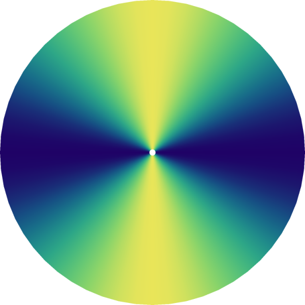
and $U^{\mu}=(1,0,0,0)$ is the 4-vector of a static observer in Poincaré coordinates. The result is accessible at [18]. Figure 1 contains screenshots of the simulations at $t=0$. Likewise, we also animated the energy and angular momentum currents $\mathcal{I}^{E}$ and $\mathcal{I}^{L}$. Figure 4 depicts screenshots of these simulations at $t=0$. In all these figures, the color scheme is in natural units.

Finally, we also animated the flow of the current $\mathcal{J}$. Figure 5 depicts screenshots of the simulations at $t=0$ and at $t=5$.

For the solutions $\Re F_{(h,0)}$, the energy and angular momentum fluxes (3.38) at the horizon are

$\displaystyle\mathcal{E}_{H}^{\pm}=\pm 2\sqrt{2}\Lambda\left[P_{h}^{\prime}\left(\sin{\pm\tau}\right)^{h+1}\cos{(h+1)\tau}\right]^{2},\qquad\mathcal{L}_{H}^{\pm}=0.$

(5.22)

Likewise, for the solutions $\Im F_{(h,0)}$,

$\displaystyle\mathcal{E}_{H}^{\pm}=\pm 2\sqrt{2}\Lambda\left[P_{h}^{\prime}\left(\sin{\pm\tau}\right)^{h+1}\sin{(h+1)\tau}\right]^{2},\qquad\mathcal{L}_{H}^{\pm}=0.$

(5.23)

In both cases, the fluxes out of the boundary of NHEK vanish for $h>\frac{1}{2}$:

$\displaystyle\mathcal{E}_{\infty}=\mathcal{L}_{\infty}=0,$

(5.24)

Plugging these expressions into (3.35) yields

$\displaystyle\Delta E_{H}^{+}=-\Delta E_{H}^{-},\qquad\Delta E_{B}=0,$

(5.25)

which is of course consistent with (3.34). This case is illustrated in Figure 6. On the other hand, when $h<\frac{1}{2}$, the energy flux density $\mathcal{E}_{\infty}$ at the boundary becomes divergent. For the boundary case $h=\frac{1}{2}$, it is nonzero but finite: for the solutions $\Re F_{(1/2,0)}$,

$\displaystyle\mathcal{E}_{\infty}=2\sqrt{2}\,\Lambda\,{P_{1/2}^{\prime}}^{2}(1+\cos\tau)\sin{\tau}\cos^{2}{\frac{\tau}{2}},$

(5.26)

while for the solutions $\Im F_{(1/2,0)}$,

$\displaystyle\mathcal{E}_{\infty}=-2\sqrt{2}\,\Lambda\,{P_{1/2}^{\prime}}^{2}\cos\tau\sin{\tau}\cos^{2}{\frac{\tau}{2}}.$

(5.27)

In either situation, the total flux through the boundary $\Delta E_{B}$ is still zero, which is consistent with the fact that the energy flux out of the future horizon equals that into the past horizon.

Finally, note from (5.22) and (5.23) that the total horizon fluxes $\Delta E_{H}^{\pm}$ are only finite when $h\geq-1$. For $h<-1$, even though these quantities diverge, the relation $\Delta E_{H}^{+}=\Delta E_{H}^{-}$ still holds.

Consider the Ansatz

$\displaystyle A_{(1,0)}=\Psi\Lambda\tilde{P}\,\mathrm{d}\theta,$

(6.1)

where in the last line we introduced a scalar function

$\displaystyle\Psi(\tau,\psi)\equiv-e^{-i(\tau+\psi)},$

(6.2)

while $\tilde{P}(\theta)$ can be an arbitrary regular function. $\Psi(\tau,\psi)$ is a $\mathsf{U}(1)\times\mathsf{U}(1)$ eigenfunction

	$\displaystyle\mathcal{L}_{L_{0}}\Psi$	$\displaystyle=\Psi,$		(6.3)
	$\displaystyle\mathcal{L}_{Q_{0}}\Psi$	$\displaystyle=0.$		(6.4)

However, it does not lie in a scalar highest-weight representation of $\mathsf{SL}(2,\mathbb{R})$ because it is not annihilated by $L_{+}$. Instead, it obeys

$\displaystyle\mathcal{L}_{L_{+}}\Psi=1.$

(6.5)

Note also that is just a complex phase: $\Psi^{*}\Psi=1$. It follows that $A_{(1,0)}$ obeys

	$\displaystyle\mathcal{L}_{L_{+}}A_{(1,0)}$	$\displaystyle=\Psi^{*}A_{(1,0)}=\Lambda\tilde{P}\,\mathrm{d}\theta,$		(6.6)
	$\displaystyle\mathcal{L}_{L_{0}}A_{(1,0)}$	$\displaystyle=A_{(1,0)},$		(6.7)
	$\displaystyle\mathcal{L}_{Q_{0}}A_{(1,0)}$	$\displaystyle=0.$		(6.8)

Observe that it is annihilated by $L_{+}$ up to a gauge transformation. The corresponding 2-form field strength $F_{(1,0)}\equiv\,\mathrm{d}A_{(1,0)}$ is

	$\displaystyle F_{(1,0)}$	$\displaystyle=-i\Psi\Lambda\tilde{P}\,\mathrm{d}\theta\wedge(\,\mathrm{d}\tau+\,\mathrm{d}\psi)$		(6.9)
		$\displaystyle=\frac{i\Phi\Lambda\tilde{P}}{2J\Gamma}\,\mathrm{d}\theta\wedge\left(\Psi L_{+}-L_{0}-Q_{0}\right),$		(6.10)

where $\Phi(\tau,\psi)$ is defined in (4.3). From (6.9), it is easily checked that $\mathcal{L}_{L_{+}}F_{(1,0)}=0$, which together with (6.7)–(6.8) implies that $F_{(1,0)}$ is $U(1)$-invariant and forms a highest-weight representation of $\mathsf{SL}(2,\mathbb{R})$ with highest weight $h=1$. The associated current $\mathcal{J}_{(1,0)}\equiv\,\mathrm{d}^{\dagger}F_{(1,0)}$ is given by

	$\displaystyle\mathcal{J}_{(1,0)}$	$\displaystyle=\frac{i\Psi\left(\Lambda\tilde{P}^{\prime}+2\Lambda^{\prime}\tilde{P}\right)}{2J\Gamma}\left(\,\mathrm{d}\tau+\,\mathrm{d}\psi\right)$		(6.11)
		$\displaystyle=\frac{i\Phi\left(\Lambda\tilde{P}^{\prime}+2\Lambda^{\prime}\tilde{P}\right)}{(2J\Gamma)^{2}}\left(\Psi L_{+}-L_{0}+Q_{0}\right).$		(6.12)

while

	$\displaystyle\star F_{(1,0)}$	$\displaystyle=-i\Psi\Lambda^{2}\tilde{P}\left[\cot{\psi}\,\mathrm{d}\tau\wedge\,\mathrm{d}\psi+\left(\,\mathrm{d}\tau+\,\mathrm{d}\psi\right)\wedge\,\mathrm{d}\varphi\right]$		(6.13)
		$\displaystyle=\frac{i\Phi\tilde{P}}{(2J\Gamma)^{2}}Q_{0}\wedge\left(\Psi L_{+}-L_{0}+Q_{0}\right).$		(6.14)

Since both are proportional to $\,\mathrm{d}\tau+\,\mathrm{d}\psi$ (or $\Psi L_{+}-L_{0}+Q_{0}$)

$\displaystyle\mathcal{J}_{(1,0)}\wedge\star F_{(1,0)}=0$

(6.15)

and $F_{(1,0)}$ is a force-free solution. Note that it is null in the sense that

$\displaystyle F_{(1,0)}^{2}=0.$

(6.16)

The stress energy-momentum tensor of this solution takes the simple form

$\displaystyle T_{(1,0)}^{\mu\nu}=2J\Gamma\left(\frac{\Lambda\tilde{P}}{\Lambda\tilde{P}^{\prime}+2\Lambda^{\prime}\tilde{P}}\right)^{2}\mathcal{J}_{(1,0)}^{\mu}\mathcal{J}_{(1,0)}^{\nu}.$

(6.17)

Hence we may interpret this solution as describing a pressureless perfect fluid.

References

- [1] A. Hewish, J. D. H. Pilkington, P. F. Scott, and R. A. Collins, ”Observation of a Rapidly Pulsating Radio Source,” Nature 217: 709 (1968)
- [2] T. A. Matthews and A. R. Sandage, Optical Identification of 3c 48, 3c 196, and 3c 286 with Stellar Objects. Astrophys. J. 138, 30 (1963)
- [3] R. D. Blandford and R. L. Znajek, “Electromagnetic extractions of energy from Kerr black holes,” Mon. Not. Roy. Astron. Soc. 179, 433 (1977).
- [4] T. D. Brennan, S. E. Gralla and T. Jacobson, “Exact Solutions to Force-Free Electrodynamics in Black Hole Backgrounds,” Class. Quant. Grav. 30, 195012 (2013) [arXiv:1305.6890 [gr-qc]].
- [5] F. C. Michel “Rotating Magnetospheres: An Exact 3-D Solution,” Astroph. J. 180, 133 (1973).
- [6] R. D. Blandford, Monthly Notices of the Royal Astronomical Society 176 465–481 (1976).
- [7] G. Menon and C. D. Dermer, General Relativity and Gravitation 39 (2007). 785–794
- [8] K. Tanabe and S. Nagataki, “Extended monopole solution of the Blandford-Znajek mechanism: Higher order terms for a Kerr parameter,” Phys. Rev. D 78, 024004 (2008) [arXiv:0802.0908 [astro-ph]].
- [9] T. D. Brennan and S. E. Gralla, Phys. Rev. D 89, no. 10, 103013 (2014) [arXiv:1311.0752 [astro-ph.HE]].
- [10] S. E. Gralla and T. Jacobson, “Spacetime approach to force-free magnetospheres,” arXiv:1401.6159 [astro-ph.HE].
- [11] L. Gou, J. E. McClintock, R. A. Remillard, J. F. Steiner, M. J. Reid, J. A. Orosz, R. Narayan and M. Hanke et al., arXiv:1308.4760 [astro-ph.HE].
- [12] J. M. Bardeen and G. T. Horowitz, “The Extreme Kerr throat geometry: A Vacuum analog of AdS(2) x S**2,” Phys. Rev. D 60, 104030 (1999) [hep-th/9905099].
- [13] M. Guica, T. Hartman, W. Song and A. Strominger, “The Kerr/CFT Correspondence,” Phys. Rev. D 80, 124008 (2009) [arXiv:0809.4266 [hep-th]].
- [14] I. Bredberg, C. Keeler, V. Lysov and A. Strominger, Nucl. Phys. Proc. Suppl. 216, 194 (2011) [arXiv:1103.2355 [hep-th]].
- [15] A. P. Porfyriadis and A. Strominger, arXiv:1401.3746 [hep-th].
- [16] S. Hadar, A. P. Porfyriadis and A. Strominger, arXiv:1403.2797 [hep-th].
- [17] A. Lupsasca and M. J. Rodriguez, in progress.
- [18] http://www.youtube.com/playlist?list=PLsrfyTK-g7cP-_8F7A5Zb71K_94_gaXgn
- [19] S. S. Komissarov, “On the properties of time dependent, force-free, degenerate electrodynamics,” Mon. Not. Roy. Astron. Soc. 336, 759 (2002) [astro-ph/0202447].
- [20] S. M. Carroll, “Lecture notes on general relativity,” gr-qc/9712019.
- [21] N. Ja. Vilenkin and A. U. Klimyk, “Representation of Lie groups and special functions,” Math. Appl., Kluwer Acad. Publ., Dordrecht, Vols. 1–3.
- [22] J.-P. Lasota, E. Gourgoulhon, M. Abramowicz, A. Tchekhovskoy and R. Narayan, Phys. Rev. D 89, 024041 (2014) [arXiv:1310.7499 [gr-qc]].