Eclipse Hashing: Alexandrov Compactification and
Hashing with Hyperspheres for Fast Similarity Search

Yui Noma Note: Software Systems Laboratories, FUJITSU LABORATORIES LTD. 1-1, Kamikodanaka 4-chome, Nakahara-ku Kawasaki, 211-8588 Japan. Note: E-mail: noma.yui@jp.fujitsu.com Makiko Konoshima ¹¹footnotemark: 1 Note: E-mail: makiko@jp.fujitsu.com

Abstract

The similarity searches that use high-dimensional feature vectors consisting of a vast amount of data have a wide range of application. One way of conducting a fast similarity search is to transform the feature vectors into binary vectors and perform the similarity search by using the Hamming distance. Such a transformation is a hashing method, and the choice of hashing function is important.

Hashing methods using hyperplanes or hyperspheres are proposed. One study reported here is inspired by Spherical LSH [1], and we use hypersperes to hash the feature vectors.

Our method, called Eclipse-hashing, performs a compactification of $\mathbb{R}^{n}$ by using the inverse stereographic projection, which is a kind of Alexandrov compactification. By using Eclipse-hashing, one can obtain the hypersphere-hash function without explicitly using hyperspheres. Hence, the number of nonlinear operations is reduced and the processing time of hashing becomes shorter. Furthermore, we also show that as a result of improving the approximation accuracy, Eclipse-hashing is more accurate than hyperplane-hashing.

Keywords: Locality-sensitive hashing, Hypersphere, Alexandrov compactification, Inverse stereographic projection.

1 Introduction

At present, there are great opportunities for those who can make good use of unstructured data, such as images, movies, and data captured by sensors. Among the available utilities for dealing with unstructured data, similarity searches have a wide range of application. For example, similarity searches of images obtained by scanning biometric information are used for card-less micropayments and fraud detection. Moreover, many similarity search methods work by extracting feature vectors from unstructured data. These feature vectors reflect the complexity of the data from which they were extracted and can have hundreds or even thousands of dimension.

One also needs to retrieve data from tens millions or even billions of records. In addition, to utilize the unstructured data, one has to associate it with existing structured data. Furthermore, by taking the need for security into consideration, it is preferable to store such data in a database (DB).

If one does a similarity search naively, the processing time is proportional to the number of records. Hence, a naive similarity search conducted on a huge amount of records takes a very long time. Because of this, fast similarity search methods have been developed, and many index structures have been proposed for them. Two such indexes are R-Tree [2] and kd-tree [3]. Moreover, to utilize unstructured data, one needs an index structure that permits fast similarity searches in a high-dimensional space. However, such index structures have yet to be developed.

The system requirements of the actual applications of unstructured data can be met not only by the similarity searches but also by approximate-similarity searches. Let us take the case of a card-less micropayment system that uses biometric information images as an example. Here, a customer who wants to make a payment scans his biometric information image in a shop. The image is sent to the micropayment system. The system does a fast (approximate) similarity search of the images and finds two or more images that are similar to the query image from the database that stores one thousand images. The similar images are sent to the biometric authentication engine, which is an accurate and heavy process, and the engine returns the person’s ID. The system then performs the payment process. For such processes, one needs a fast and accurate biometric authentication system (Please see the literature [4] for details). If one needs higher accuracy, the biometric authentication engine and/or the approximate-similarity search have to be refined.

We took recent developments in memory technologies into consideration and paid attention to the following technique with high compatibility with in-memory DBs. The method performs similarity searches by converting the feature vectors to bit-vectors and using the Hamming distance to represent the dissimilarities between the bit-vectors. This method has been used, for example, in content-based image retrieval systems [5, 6, 7, 8]. Since the Hamming distance calculation is much faster than the $L_{2}$ distance calculation of the feature vectors, a similarity search in Hamming distance space is very fast. Furthermore, since the information in the feature vectors is represented with bit-vectors that are smaller than the feature vectors, information on a large amount of unstructured data can be loaded into memory. However, since the hashing causes a loss of information, similarity searches using bit-vectors are approximations of ones using feature vectors. To improve the accuracy, one might try lengthening the bit-vectors. However, a huge amount of very long bit-vectors cannot be stored in memory. Therefore, one has to devise a hashing method that produces an accurate approximate-similarity search with bit-vectors that are not too long.

The hashing methods that use hyperplanes are locality-sensitive hashings and are actively studied [9, 10, 11, 12, 13, 4, 14, 5, 7, 15, 16]. Interpreting these hashing methods from a geometrical viewpoint, we can see that they use a hyperplane to divide the feature vector space into two regions, and assign $0$ or $1$ to each region and the vectors contained in them. The bit is determined by the orientation of the hyperplane. By performing this operation many times, they assign bit-vectors to the feature vectors. In contract, in the case of a feature vector space is a $L_{2}$ metric space, it is natural to divide up the space by using hyperspheres instead of hyperplanes because the distance between feature vectors in a hypersphere is less than the diameter. Therefore, it is expected that a hypersphere-hashing approximation would be more accurate than a hyperplane-hashing approximation. A hashing method using hyperspheres was first proposed in [1].

Hashing with a kernel has also been proposed [17, 18]. We can use kernels to divide up a space with complicated hypersurfaces, and this is expected to yield a more accurate approximation than that of hyperplane hashing. Despite this, it noted in [1] that many separate regions may have a same bit-vector. Furthermore, it is hard to control the generation of such regions. Hence, the accuracy of the hashing with a kernel approximation would deteriorate in such cases.

The following two problems occur when we naively do the hashing with hyperspheres explained in detail in section 3.1. The first problem is an effect caused by the existence of a shortcut through a neighborhood around the infinity. The second problem is the occurrence of the destruction of localities.

We propose a new hashing scheme in this paper, called Eclipse-hashing. Eclipse-hashing uses the inverse stereographic projection to solve the above-mentioned problems.

2 Related work

Here, we explain methods that are related ours. We will assume that the feature space is an $L_{2}$ distance space.

2.1 Hashing with hyperplanes

Let the feature space $V$ be an $N$ -dimensional space, i.e., $\mathbb{R}^{N}$ , and let $(x_{1},x_{2},\cdots,x_{N})$ be the coordinates of a vector in $V$ . A hyperplane that crosses the origin of $V$ is called a linear hyperplane. Otherwise, it is called an affine hyperplane. Consider $B$ hyperplanes $\{H^{(k)}\}_{k=1,\cdots,B}$ in $V$ . By letting $\{\vec{n}^{(k)}\}_{k=1,\cdots,B}$ be the unit normal vectors of $H^{(k)}$ and $\{b^{(k)}\}_{k=1,\cdots,B}$ be the offset, the equation of $H^{(k)}$ can be formulated as follows:

\displaystyle\phi^{(k)}(\vec{x})=\vec{n}^{(k)}\cdot\vec{x}+b^{(k)}.

(1)

When the hyperplane $H^{(k)}$ is linear, $b^{(k)}=0$ . The hash function defined by the $k$ -th hyperplane is given¹¹ 1 This hash function corresponds to the limit where $r\rightarrow\infty$ of the hash function in [9]. :

\displaystyle h^{(k)}(\vec{x})=\begin{cases}1&\text{if $\vec{n}^{(k)}\cdot\vec{x}+b^{(k)}>0$,}\\ 0&\text{otherwise.}\end{cases}

(2)

Since this hash function is a linear operation, it is fast. The bit-vector assigned to $\vec{x}$ is $\vec{h}(\vec{x})=(h^{(1)}(\vec{x}),\cdots,h^{(B)}(\vec{x}))$ .

The details of the hash functions depend on the normal vectors. There are many ways to give the normal vectors: by sampling them randomly from a multi-dimensional standard normal distribution [12], using PCA [19], or by using the density of data [15]. When labeled data are attached to the feature vectors, one can find the normal vector by using supervised learning: S-LSH [4], M-LSH [13], MLH [14].

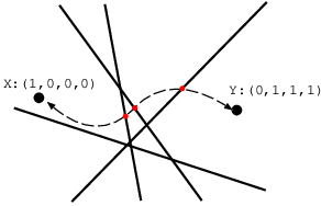
From a geometrical viewpoint, the operation of the hash functions $h^{(k)}$ corresponds to using $B$ hyperplanes to divide up the feature space and assigning the bit-vectors to the feature vectors. The Hamming distance between the bit-vectors converted from two feature vectors corresponds to the minimum of the number of intersections between the hyperplanes and the path connecting the two feature vectors. We illustrate the correspondence in Fig. 1.

Refer to caption — Figure 1: Correspondence between the minimum number of intersections and the Hamming distance. The number of intersections is defined by the number of crossing points of the hyperplanes and the path connecting $X$ and $Y$ .

2.2 Hashing methods related to hyperspheres

Let us explain the existing hashing methods that are related to hyperspheres. In spherical hashing [1], one considers multiple hyperspheres in the feature space and assigns $1$ to the feature vectors if they are in the sphere and $0$ , otherwise. The similarities between the bit-vectors, however, are not computed with the Hamming distance, but with the spherical-Hamming distance defined by the following equation:

	$\displaystyle\mathrm{SphericalHammingDist}(b1,b2)$
	$\displaystyle:=\|\mathrm{xor}(b1,b2)\|/\|\mathrm{and}(b1,b2)\|,$		(3)

where $|v|$ indicates counting the number of $1$ s in the bit-vector $v$ . The spherical-Hamming distance, however, causes division by $0$ and the indeterminant $\frac{0}{0}$ . Therefore, the spherical-Hamming distance is not an appropriate way to determine the similarities between bit-vectors.

Another hashing method related to hyperspheres is Spherical LSH [20]. This method is not a hashing method with hyperspheres but rather one with feature vectors located on a unit sphere in the feature space. It uses high-dimensional regular polytopes. The hash function assigns the ID of the vertex of the polytope to the feature vectors. Hence, the hash value is not a bit-vector.

3 Eclipse-hashing

3.1 Motivation

When the feature space is an $L_{2}$ distance space, hashing with hyperspheres [1] is a natural idea. However, because of the discussion in section 2.2, we use the Hamming distance to calculate the similarities between the bit-vectors instead of the spherical-Hamming distance.

Let us consider hashing with hyperspheres. Suppose we have $B$ hyperspheres and denote the center of the $k$ -th hypersphere as $\vec{p}_{\mathrm{HS}}^{(k)}$ and the radius as $r_{\mathrm{HS}}^{(k)}$ . The naive hashing is as follows:

\displaystyle h_{\mathrm{HS}}^{(k)}(\vec{x})=\begin{cases}1&\text{if $\sum_{i=1}^{B}(x_{i}-(p_{\mathrm{HS}}^{(k)})_{i})^{2}<r_{\mathrm{HS}}^{(k)}$,}\\ 0&\text{otherwise.}\end{cases}

(4)

Keeping in mind that the normal vectors are given randomly in [9], we set the position and radius randomly in section 4.

Although it is not described in [1], we should point that there are two problems related to naive hashing with hyperspheres.

-Problem 1: Effect of a shortcut through a neighborhood of the infinity. Let us consider the regions $R1$ and $R2$ in $V$ , as shown in Fig. 2. Since the bit-vectors assigned to them are the same, the Hamming distance between the points selected from each region is zero. This means that path $P2$ is shorter than $P1$ . Hence, the accuracy of the approximation deteriorates. $P2$ can be seen as a shortcut through the neighborhood of the infinity from the viewpoint of projective geometry.

-Problem 2: Disconnectivity of regions with the same bit-vector. Let us consider a case in which the feature space $V$ is two dimensional and the hashing is with three spheres, as shown in Fig. 4. The bit-vectors assigned to the regions $R3$ and $R4$ are the same, $(0,0,0)$ . In contrast, the region having the bit-vector $(0,0,0)$ is disconnected. In this case, the Hamming distance between the bit-vectors corresponding to $a\in R3$ and $b\in R4$ is zero.

However, any path connecting $a$ and $b$ intersects the spheres. Therefore, the Hamming distance is different from the minimum number of intersections between the path and the spheres. Because of this mismatch, one can not approximate the $L_{2}$ distance by the Hamming distance.

We interpret this phenomenon as follows. If a path connecting $a$ and $b$ does not exist in the space $V$ and, except for its end points, is outside $V$ , it does not intersect the spheres. Let us consider a three-dimensional ambient space in which $V$ is located as shown in the Fig. 4. The ambient space can be seen as the direct product of the space $V$ and an extra dimension. Furthermore, we consider the tube $T$ connecting $R3$ and $R4$ , as shown in Fig. 4. When a path connecting $a$ and $b$ exists in this tube, the path does not intersect the spheres. Therefore, by considering this ambient space and the tube the Hamming distance and the minimum number of intersections can be made to correspond. We call $T$ a wormhole because it is similar to the wormholes predicted by general relativity.

In general, wormholes can exist when we partition a two-dimensional space with many spheres. Similar things occur in the cases in which the dimension of the space is higher than two. That is to say, when we divide up an $N$ -dimensional space $V$ with $N+1$ hyperspheres, a region corresponding to a bit-vector can be disconnected, and wormholes can exist. Therefore, if we do the hashing with hyperspheres naively, the accuracy of the approximation deteriorates.

3.2 Our contribution

Our proposal solves the above-mentioned problems. The key idea is the use of the inverse stereographic projection. In the following we assume that the origin of $V$ and the mean vector of the feature vectors are the same.

3.2.1 Inverse stereographic projection and hyperspheres

Let us consider $\tilde{V}=\mathbb{R}^{N+1}$ , and let $(\tilde{x}_{1},\tilde{x}_{2},\cdots,\tilde{x}_{N+1})$ be the coordinate of $\tilde{V}$ . The following mapping is the so-called inverse stereographic projection $f^{-1}:V\rightarrow\tilde{V}$ .

			$\displaystyle f^{-1}(x_{1},x_{2},\cdots,x_{N};d)$		(5)
		$\displaystyle=$	$\displaystyle\left(\frac{2dx_{1}}{d^{2}+r^{2}},\cdots,\frac{2dx_{N}}{d^{2}+r^{2}},\frac{-d^{2}+r^{2}}{d^{2}+r^{2}}\right),$		(5)

where $r^{2}:=\sum_{i=1}^{N}x_{i}^{2}$ , and $d$ is a given positive real number. The image of $f^{-1}$ is a unit sphere $S$ whose center is the origin of $\tilde{V}$ , except the north pole, $(0,0,\cdots,1)$ . The function $f^{-1}$ is the inverse of the stereographic projection²² 2 The (inverse) stereographic projection is well known in mathematics. $f:S\setminus\{(0,0,\cdots,1)\}\rightarrow V$ .

The dimensionality of $S$ is $N$ . Suppose we arrange $V$ at $\tilde{x}_{N+1}=-d+1$ and consider rays whose initial point is the north pole of $S$ ; this mapping is a correspondence between the point where the ray and $S$ intersect and the intersection of the ray and $V$ . Figure 5 shows the correspondence. When we extend the domain of the mapping to contain the infinity of $V$ , the image of the infinity is the north pole of $S$ : i.e., $S$ can be identified as $V$ and the infinity, $S\cong V\cup\{\infty\}$ . This identification is a kind of Alexandroff compactification.

Let us consider a partition of the unit sphere $S$ by an affine hyperplane $\tilde{H}$ in $\tilde{V}$ . The dimensionality of $\tilde{H}$ is $N$ because it is a hyperplane in $(N+1)$ -dimensional space $\tilde{V}$ . The equation of $\tilde{H}$ is:

\displaystyle\tilde{\phi}(\tilde{x})=\vec{\tilde{n}}\cdot\vec{\tilde{x}}+\tilde{b}=0,

(6)

where $\vec{\tilde{n}}=(\tilde{n}_{1},\tilde{n}_{2},\cdots,\tilde{n}_{N+1})$ is the normal vector, and $\tilde{b}$ is the offset. If $\tilde{H}$ and $S$ have a common set, the image of the common set under the stereographic projection $f$ is as follows:

	$\displaystyle 0$	$\displaystyle=$	$\displaystyle\tilde{\phi}(f^{-1}(x;d))$		(7)
		$\displaystyle=$	$\displaystyle\sum_{i=1}^{N}\tilde{n}_{i}\frac{2dx_{i}}{d^{2}+r^{2}}+\tilde{n}_{N+1}\frac{-d^{2}+r^{2}}{d^{2}+r^{2}}+\tilde{b}$		(7)

In the case of $\tilde{n}_{N+1}=-\tilde{b}$ , we obtain the following equation from eq.(7).

\displaystyle\sum_{i=1}^{N}\tilde{n}_{i}x_{i}+d\tilde{b}=0.

(8)

This is the equation of an affine hyperplane in $V$ . In the case of $\tilde{n}_{N+1}\not=-\tilde{b}$ , we obtain

			$\displaystyle\sum_{i=1}^{N}\left(x_{i}+\frac{d\tilde{n}_{i}}{\tilde{n}_{N+1}+\tilde{b}}\right)^{2}$		(9)
		$\displaystyle=$	$\displaystyle\frac{d^{2}}{(\tilde{n}_{N+1}+\tilde{b})^{2}}\left(\sum_{i=1}^{N+1}\tilde{n}_{i}^{2}-\tilde{b}^{2}\right).$		(9)

This is the equation of a hypersphere in $V$ . Especially in the case of $\vec{\tilde{n}}=(0,\cdots,0,1)$ and $\tilde{b}=0$ , the common set is the equator $E$ of $S$ . The image of $E$ under $f$ is a hypersphere, and the radius of the hypersphere is $d$ . From the above discussion, the image of the common set of $\tilde{H}$ and $S$ under the stereographic projection is an affine hyperplane or a hypersphere. Figure 6 shows sketches of this situation.

Since the degree of freedom of a hyperplane in $\tilde{V}$ is equal to that of a hypersphere or a hyperplane in $V$ , there is a one-to-one correspondence between hyperspheres and hyperplanes in $V$ and hyperplanes in $\tilde{V}$ whose common set with $S$ are not empty. Furthermore, the two regions in $S$ separated by a hyperplane in $\tilde{V}$ and the two regions in $V$ separated by the corresponding hypersphere or hyperplane coincide because $f$ and $f^{-1}$ are continuous.

3.2.2 Solution to the problems

Since division of $S$ by hyperplanes and division of $V$ by hyperspheres correspond under $f^{-1}$ , as we mentioned in section 3.2.1, hashing with hyperplanes in $\tilde{V}$ after mapping the feature vectors to $S$ by $f^{-1}$ corresponds to hashing with the corresponding hyperspheres in $V$ .³³ 3 We need to invert the bits obtained from eq.(2) in order to equate them to the ones obtained from the composition of $f^{-1}$ and the hash function with hyperplanes in $\tilde{V}$ . By using this correspondence, we propose the following solutions to the problems mentioned in section 3.1.

- Solution 1: There are two factors contributing to the deterioration in accuracy of the approximation affected by the shortcut through the neighborhood of the infinity. The first factor is that the feature vectors that are far away from the origin of $V$ are mapped to the neighborhood of the north pole of $S$ , and the mapped points are near to each other in $\tilde{V}$ . The second factor is that unless the hyperplanes in $\tilde{V}$ do not cross the neighborhood of the north pole of $S$ , the Hamming distance of the bit-vectors assigned to the points near the north pole will be small.

If either of the two factors is resolved, the accuracy of the approximation may be improved. On the one hand, even if the features are mapped near the north pole, the Hamming distances of the corresponding bit-vectors will be large if many hyperplanes cross the neighborhood of the north pole. On the other hand, even if the hyperplanes do not cross the neighborhood of the north pole, the Hamming distances of the corresponding bit-vectors are small if the feature vectors are not mapped to the north pole. In the former case, since the hyperplanes cross near the pole, their image in $V$ under $f$ are hyperspheres with a large radius that can be approximated by hyperplanes in $V$ . Hence, we chose the latter resolution. Since the parameter $d$ of $f^{-1}$ , corresponds the the radius of $f(E)$ as mentioned in section 3.2.1, we choose a large $d$ in order to map the feature vectors to regions away from the pole.

- Solution 2: As we discussed in 3.1, the accuracy of the approximation deteriorates because of wormholes. Hence, if we could suppress the generation of wormholes or guarantee their non-existence, the accuracy would improve. To be able to do this, though, we need to understand the generation process.

Let us consider a one-dimensional feature space to simplify the discussion. In the case of $N=1$ , the region surrounded by a hypersphere is a closed segment. Figure 7 shows an example of two hyperspheres dividing up $V$ . The region having the bit-vector $(0,0)$ are disconnected. Therefore, a wormhole certainly exists. The region having the bit-vector $(0,0)$ is mapped by $f^{-1}$ to the two regions, the neighborhoods of the south and north poles. As illustrated in Fig. 7, we can connect the two regions by putting a tube $T$ through the inside of $S$ . The tube $T$ is the wormhole. By looking at figure 7, we can understand the following: the wormhole is generated because the intersection of $H1$ and $H2$ exists outside of $S$ . Hence, if the intersection exists inside or at $S$ , a wormhole would not be generated.

Although the above discussion is for the case of $N=1$ , wormholes may exist if the dimension of $V$ is greater than one: they may be generated by $N+1$ hyperspheres in a $N$ -dimensional space. However, if the intersection point of the $N+1$ hyperplanes in $\tilde{V}$ exists inside or at $S$ , a wormhole would not be formed as a result of using $N+1$ hyperplanes. When the length of the bit-vector is $B$ , there is no wormhole if all the intersections of $B$ hyperplanes in $\tilde{V}$ are inside or at $S$ . The number of intersections is $\frac{B!}{N!(B-N)!}$ , since there is one intersection for each combination of $N+1$ hyperplanes. Hence, when $N$ and $B$ are large, it is very heavy task to check all the intersection are inside or at $S$ in order to guarantee that wormholes do not exist.

One of the simplest solutions to reducing the size of the task is to require the following condition: all hyperplanes in $\tilde{V}$ cross a point that exists inside or at $S$ . We call such a point a common intersection and denote it by $C$ . Please note that all hyperplanes crossing $C$ have a common set with $S$ .

3.2.3 Eclipse-hashing

Based on the discussion in section 3.2.1 and 3.2.2, we can describe the Eclipse-hashing as follows. Map the feature vectors in $V$ to $S$ by using the inverse stereographic projection (eq.(5)). Select a common intersection $C$ inside or at $S$ . Chose the normal vectors of $B$ hyperplanes in $\tilde{V}$ that cross $C$ . Hash the mapped feature vectors by using the hashing method with hyperplanes.⁴⁴ 4 By regarding the space $V$ as a flat earth, the sphere $S$ can be seen as the moon in the universe. Dividing up the moon and assigning $0$ or $1$ to each region reminded us of a lunar eclipse. Hence, we decided to call this method Eclipse-hashing. The hash function is:

\displaystyle\tilde{h}^{(k)}(\vec{x})=\begin{cases}1&\text{if $\vec{\tilde{n}}^{(k)}\cdot(f^{-1}(\vec{x};d)-\vec{C})>0$,}\\ 0&\text{otherwise ,}\end{cases}

(10)

where $\vec{C}$ is the position vector of $C$ .

Let $W$ be a $B\times(N+1)$ matrix whose $k$ -th row vector is the normal vector $\vec{\tilde{n}}^{(k)}$ of the $k$ -th hyperplane. The pseudo-code of Eclipse-hashing is listed in Algorithm 1.

Algorithm 1 Eclipse-hashing

\vec{x},W,\vec{C},d

\vec{\tilde{x}}\leftarrow f^{-1}(\vec{x};d)

\vec{\tilde{x}}\leftarrow\vec{\tilde{x}}-\vec{C}

b\leftarrow\frac{1}{2}(1+sgn(W\vec{\tilde{x}}))

b

The parameters in Eclipse hashing are $d$ in $f^{-1}$ , the common intersection $C$ , and the normal vectors of the hyperplanes in $\tilde{V}$ . One can determine the normal vectors according to the purpose. Some of the determination methods are unsupervised learning like in the literature [12] or supervised learning [4, 13, 14]. The parameters $d$ and $C$ should be appropriately adjusted in order to solve the problems, as mentioned in section 3.2.2. We show in section 4 that the accuracy of the approximation can be improved by adjusting these parameters.

All the hash functions treated in Eclipse-hashing are expressed with hyperspheres. However, Eclipse-hashing has the following advantages:

•

By simply setting a common intersection, we can guarantee that wormholes will not exist.
•

By mapping the feature vectors to $S$ , and translating them as $C$ becomes the origin, all the hyperplanes that we are considering cross the origin of $\tilde{V}$ . Therefore, we can apply existing supervised learning methods, for example [13] [4] [14], to determine the normal vectors of hyperplanes in $\tilde{V}$ .

4 Experiments

We measured the processing time and the accuracy of the approximation of Eclipse-hashing. Furthermore, we measured the performances of the following hashing methods: $\mathrm{LH}$ ; hashing with linear hyperplanes in $V$ , $\mathrm{AH}$ ; hashing with affine hyperplanes in $V$ , and $\mathrm{HS}$ ; naive hashing with hyperspheres in $V$ . In the following, we abbreviate Eclipse-hashing as $\mathrm{EH}$ .

In order to simplify the discussion, we set $\vec{C}=(0,0,\cdots,c)$ . The condition where $c\in[-1,1]$ must be imposed to ensure that the common intersection is inside or at $S$ .

4.1 Processing time of hashing

Here, we report the processing times of hashing of all the methods. The experiment’s environment was as follows. The CPU was an Intel Xeon X5680 3.3GHz, and the size of the main memory was 32.0GB. Each method was implemented using C++, each process was a single thread, and the linear algebra library Eigen [21] was used. We used the Time Stamp Counter to measure the processing times.

The feature vectors were artificially made data that were sampled from the 512-dimensional standard normal distribution. The number of the feature vectors was 10,000. Since the processing time of $\mathrm{EH}$ does not depend on the parameters $c$ and $d$ , we set $c=0$ and $d=1$ . In addition, the normal vectors and the offsets of the hyperplanes and the centers and the radii of the hyperspheres were sampled from the 512-dimensional standard normal distribution, since they do not affect the processing times of all the methods.

Figure 8 shows the processing time of hashing with each method versus the length of the bit-vectors. The figure reveals that the processing time of $\mathrm{EH}$ is similar to that of $\mathrm{HS}$ and approaches those of $\mathrm{LH}$ and $\mathrm{AH}$ as the bit-vectors becomes longer. For example, when the length of the bit-vectors is 1,024, hashing with $\mathrm{EH}$ is about four times as fast as hashing with $\mathrm{HS}$ .

4.2 Accuracy of approximation

4.2.1 Experimental data sets

The data sets used in the experiments were MNIST [22], which is a set of the raw image data of hand-written digits, LabelMe, which is a set of Gist feature vectors [23] extracted from image data that was published in reference [8], and a set of artificial data that were sampled from the 512-dimensional standard normal distribution. Each data set was partitioned into two sets, one, the set of the data in the database, the other, the set of the data used for the queries. We shifted the feature vectors so that the mean vectors of the data sets were zero vectors. The data sets are summarized in Table 1. The length of the bit-vectors was 1,024.

Table 1: Quantities of the data sets

	MNIST	LabelMe	Artificial data
Number of data for records	60,000	11,000	10,000
Number of data for queries	10,000	11,000	1,000
Dimensionality	784	512	512

4.2.2 Details of the experiment

We used the mean of recalls as an indicator to measure the accuracy of the approximation. Let $Z(q,k)$ be the $k$ -nearest neighbors for a query $q$ . By converting the feature vectors with each method, we denote $W(q,k;\mathrm{Meth})$ as the $k$ -nearest neighbors for a query $q$ in the Hamming space, where $\mathrm{Meth}=\mathrm{LH},\mathrm{AH},\mathrm{HS},\mathrm{EH}$ . The indicator is

	$\displaystyle\mathrm{Recall}(k;\mathrm{Meth}):=$
	$\displaystyle\frac{1}{\#(Q)}\sum_{q\in Q}\frac{\#(Z(q,k)\cap W(q,k;\mathrm{Meth}))}{k},$		(11)

where $Q$ is the set of queries. In the following, we equated $k$ to the $1\%$ of the number of the record data.

The hyperplanes and hyperspheres for each method were set as follows. The normal vectors of the hyperplanes for $\mathrm{EH}$ were sampled from the $(N+1)$ -dimensional standard normal distribution. The normal vectors of the hyperplanes for $\mathrm{LH}$ were sampled from the $N$ -dimensional standard normal distribution. For $\mathrm{AH}$ , the normal vectors of the hyperplanes were sampled from the $N$ -dimensional standard normal distribution, and the offsets of the hyperplanes were sampled from a uniform distribution whose support was $[0,1]$ . The centers of the hyperspheres for $\mathrm{HS}$ were sampled from the $N$ -dimensional standard normal distribution, and the radii of the hyperspheres were $\sqrt{N}$ times the absolute values of values sampled from the standard normal distribution.⁵⁵ 5 The mean distance between the origin and values sampled from the $N$ -dimensional standard normal distribution is about $\sqrt{N}$ . Hence, the chosen hyperspheres partition the space near the origin of $V$ .

4.2.3 Results of the experiment

Fig. 9 shows $\mathrm{Recall}$ of each method for the artificial data. Since $\mathrm{Recall}(k;\mathrm{LH})$ , $\mathrm{Recall}(k;\mathrm{AH})$ , and $\mathrm{Recall}(k;\mathrm{HS})$ do not depend on $d$ , they are drawn as straight lines. $\mathrm{Recall}(k;\mathrm{HS})$ was close to zero. Hence, $\mathrm{HS}$ had very bad accuracy on this data set. $\mathrm{Recall}(k;\mathrm{AH})$ and $\mathrm{Recall}(k;\mathrm{LH})$ were almost the same. Furthermore, $\mathrm{Recall}(k;\mathrm{EH})$ was greater than $\mathrm{Recall}(k;\mathrm{LH})$ and $\mathrm{Recall}(k;\mathrm{AH})$ when $d$ was about $30$ and $c$ was about $0.0$ . This means that the accuracy of $\mathrm{EH}$ is higher than $\mathrm{LH}$ and $\mathrm{AH}$ with an appropriate choice of parameters.

Figure 10 shows the accuracy of the approximation of each method for MNIST and LabelMe. From these figures, we can see that $\mathrm{Recall}(k;\mathrm{HS})$ are close to zero, and there are regions of $d$ and $c$ where $\mathrm{Recall}(k;\mathrm{EH})$ are greater than $\mathrm{Recall}(k;\mathrm{LH})$ and $\mathrm{Recall}(k;\mathrm{AH})$ .

5 Discussion

The results in section 4.2.3 revealed that for all the data sets there are regions of $d$ and $c$ where $\mathrm{Recall}(k;\mathrm{EH})\approx\mathrm{Recall}(k;\mathrm{LH})$ , $\mathrm{Recall}(k;\mathrm{EH})$ is greater than $\mathrm{Recall}(k;\mathrm{LH})$ and $\mathrm{Recall}(k;\mathrm{AH})$ , and regions where $\mathrm{Recall}(k;\mathrm{EH})$ is less than $\mathrm{Recall}(k;\mathrm{LH})$ and $\mathrm{Recall}(k;\mathrm{AH})$ . Here, we will discuss the accuracies in the former two regions in this section. The last one is the complement of the former two. Moreover, we discuss the bad accuracies of $\mathrm{HS}$ .

First, let us discuss the accuracies of $\mathrm{EH}$ on in the regions where $\mathrm{Recall}(k;\mathrm{EH})\approx\mathrm{Recall}(k;\mathrm{LH})$ . When $d$ is much smaller than $r$ of the feature vectors, eq.(5) is approximated as

\displaystyle f^{-1}(x_{1},x_{2},\cdots,x_{N};d)\approx\left(\frac{2x_{1}d}{r^{2}},\cdots,\frac{2x_{N}d}{r^{2}},1\right).

(12)

Hence, the feature vectors are mapped to the neighborhood of the north pole of $S$ . In the case of $c=1$ , since all the hyperplanes in $\tilde{V}$ cross the north pole the hashing are almost similar to the hashing with hyperplanes in $V$ . Therefore, over the region where $d\ll r$ and $c\approx 1$ the accuracies of $\mathrm{EH}$ is similar to the ones of $\mathrm{LH}$ .

When $d$ is much greater than $r$ of the feature vectors the eq.(5) is approximated as follows:

\displaystyle f^{-1}(x_{1},x_{2},\cdots,x_{N};d)\approx\left(\frac{2x_{1}}{d},\cdots,\frac{2x_{N}}{d},-1\right).

(13)

Hence, the feature vectors are mapped to the neighbors of the south pole of $S$ . Since in the case of $c=-1$ all the hyperplanes in $\tilde{V}$ cross the south pole, the hashings are similar to hashing with hyperplanes in $V$ . Therefore, in the region where $d\gg r$ and $c\approx-1$ , the accuracies of $\mathrm{EH}$ are similar to those of $\mathrm{LH}$ .

Second, let us discuss the accuracies of $\mathrm{EH}$ in the regions where $\mathrm{Recall}(k;\mathrm{EH})>\mathrm{Recall}(k;\mathrm{LH})$ . Here, we define the optimal $c$ and $d$ as

\displaystyle(c_{\mathrm{opt}},d_{\mathrm{opt}}):=\arg\max_{(c,d)}(\mathrm{Recall}(k;\mathrm{EH})).

(14)

From Fig. 9 and Fig. 10, we can see that $c_{\mathrm{opt}}$ is in $[-0.5,0.5]$ and does not depend greatly on the data sets. In contrast, $d_{\mathrm{opt}}$ depends on the data sets. In the following, we experimentally show that $d_{\mathrm{opt}}$ approximately corresponds to a value for which almost all feature vectors are mapped to the south hemisphere of $S$ . In other words, we consider that solution 1 in section 3.2.2 improves the accuracies.

We calculated the ratio $\mathrm{Ratio}(d)$ of the data mapped to the south hemisphere of $S$ to the whole data. Figure 11 shows the dependency of $\mathrm{Ratio}(d)$ on $d$ .

That $\mathrm{Ratio}(d)$ is almost equal to 1 means almost all of the feature vectors are mapped to the south hemisphere. Let $d_{*}$ be the value at which $\mathrm{Ratio(d)}$ becomes greater than $0.99$ : $d_{*}:=\arg\inf_{d}(\mathrm{Ratio}(d)>0.99)$ Table 2 shows $d_{*}$ and $d_{\mathrm{opt}}$ for each data set. From the figure, we can see that $d_{\mathrm{opt}}$ have the same order as $d_{*}$ and are greater than $d_{*}$ . Therefore, almost all the feature vectors were mapped to the south hemisphere at $d_{\mathrm{opt}}$ .

Table 2:

d_{*}

and

d_{\mathrm{opt}}

	$d_{*}$	$d_{\mathrm{opt}}$
Artificial data set	27.86	32.00
MNIST	2,702	3,104
LabelMe	1.32	1.51

Finally, we discuss the bad accuracies of $\mathrm{HS}$ on all the data sets. For all the data sets, $\mathrm{Recall}(k;\mathrm{HS})$ are close to zero and much less than $\mathrm{Recall}(k;\mathrm{EH})$ with any parameters. We conclude that the deterioration in accuracy of $\mathrm{HS}$ is caused not only by the effects of shortcuts through the neighborhood of the infinity but also by wormholes.

6 Summary and future work

We proposed a new hashing scheme, called Eclipse-hashing, that leverages the inverse stereographic projection. By setting the parameters properly, we showed that the Eclipse-hashing approximation is more accurate than hashing with hyperplanes. Although hashing with hyperspheres is inaccurate in most cases and Eclipse-hashing is a kind of the hashing with hyperspheres, its accuracy was improved. We think that the reason for this improvement is that it became easy to specify the cause of the performance deterioration by using the inverse stereographic projection.

For data sets that are different from the ones used in this paper, the optimal values of $\vec{C}$ and $d$ may be different from the ones presented here. However, the discussion in section 5 suggests that $\vec{C}$ may be near the center of $S$ , and $d$ may be the value at which almost all the feature vectors are mapped to the south hemisphere.

References

[1] Jae-Pil Heo, Youngwoon Lee, Junfeng He, Shih-Fu Chang, and Sung-Eui Yoon. Spherical hashing. In CVPR, pages 2957–2964, 2012.
[2] Antonin Guttman. R-trees: A dynamic index structure for spatial searching. In Proceedings of the 1984 ACM SIGMOD International Conference on Management of Data, SIGMOD ’84, pages 47–57, New York, NY, USA, 1984. ACM.
[3] Sunil Arya, David M. Mount, Nathan S. Netanyahu, Ruth Silverman, and Angela Y. Wu. An optimal algorithm for approximate nearest neighbor searching fixed dimensions. J. ACM, 45(6):891–923, nov 1998.
[4] Makiko Konoshima and Yui Noma. Locality-sensitive hashing with margin based feature selection. arXiv:1209.5833, 2012.
[5] Jun Wang, Sanjiv Kumar, and Shih-Fu Chang. Semi-supervised hashing for scalable image retrieval. In CVPR, pages 3424–3431. IEEE, 2010.
[6] Yu-Gang Jiang, Jun Wang, and Shih-Fu Chang. Lost in binarization: query-adaptive ranking for similar image search with compact codes. In Proceedings of the 1st ACM International Conference on Multimedia Retrieval, ICMR ’11, pages 16:1–16:8, New York, NY, USA, 2011. ACM.
[7] Jun Wang, Sanjiv Kumar, and Shih-Fu Chang. Sequential projection learning for hashing with compact codes. In Johannes Furnkranz and Thorsten Joachims, editors, ICML, pages 1127–1134. Omnipress, 2010.
[8] Antonio Torralba, Rob Fergus, and Yair Weiss. Small codes and large image databases for recognition. In In Proceedings of the IEEE Conf on Computer Vision and Pattern Recognition, 2008.
[9] Mayur Datar, Nicole Immorlica, Piotr Indyk, and Vahab S. Mirrokni. Locality-sensitive hashing scheme based on p-stable distributions. In Proceedings of the Twentieth Annual Symposium on Computational Geometry, SCG ’04, pages 253–262, New York, NY, USA, 2004. ACM.
[10] Piotr Indyk and Rajeev Motwani. Approximate nearest neighbors: towards removing the curse of dimensionality. In Proceedings of the thirtieth annual ACM symposium on Theory of computing, STOC ’98, pages 604–613, New York, NY, USA, 1998. ACM.
[11] Aristides Gionis, Piotr Indyk, and Rajeev Motwani. Similarity search in high dimensions via hashing. In Proceedings of the 25th International Conference on Very Large Data Bases, VLDB ’99, pages 518–529, San Francisco, CA, USA, 1999. Morgan Kaufmann Publishers Inc.
[12] Moses S. Charikar. Similarity estimation techniques from rounding algorithms. In Proceedings of the thiry-fourth annual ACM symposium on Theory of computing, STOC ’02, pages 380–388, New York, NY, USA, 2002. ACM.
[13] Yui Noma and Makiko Konoshima. Markov chain monte carlo for arrangement of hyperplanes in locality-sensitive hashing. Journal of Information Processing, 22(1):44–55, 2014.
[14] Mohammad Norouzi and David J. Fleet. Minimal loss hashing for compact binary codes. In Lise Getoor and Tobias Scheffer, editors, ICML, pages 353–360. Omnipress, 2011.
[15] Z. Jin, C. Li, Y. Lin, and D. Cai. Density sensitive hashing. Cybernetics, IEEE Transactions on, PP(99):1–1, 2013.
[16] Yadong Mu, Xiangyu Chen, Tat-Seng Chua, and Shuicheng Yan. Learning reconfigurable hashing for diverse semantics. In Proceedings of the 1st ACM International Conference on Multimedia Retrieval, ICMR ’11, pages 7:1–7:8, New York, NY, USA, 2011. ACM.
[17] Brian Kulis and Kristen Grauman. Kernelized locality-sensitive hashing for scalable image search. In IEEE International Conference on Computer Vision ICCV, 2009.
[18] Shih-Fu Chang, Yu-Gang Jiang, Rongrong Ji, Jun Wang, and Wei Liu. Supervised hashing with kernels. 2013 IEEE Conference on Computer Vision and Pattern Recognition, 0:2074–2081, 2012.
[19] Xin-Jing Wang, Lei Zhang, Feng Jing, and Wei-Ying Ma. Annosearch: Image auto-annotation by search. In Proceedings of the 2006 IEEE Computer Society Conference on Computer Vision and Pattern Recognition - Volume 2, CVPR ’06, pages 1483–1490, Washington, DC, USA, 2006. IEEE Computer Society.
[20] Kengo Terasawa and Yuzuru Tanaka. Spherical lsh for approximate nearest neighbor search on unit hypersphere. In Frank K. H. A. Dehne, Jorg-Rudiger Sack, and Norbert Zeh, editors, WADS, volume 4619 of Lecture Notes in Computer Science, pages 27–38. Springer, 2007.
[21] Gaël Guennebaud, Benoît Jacob, et al. Eigen v3. http://eigen.tuxfamily.org, 2010.
[22] The MNIST database of handwritten digits. http://yann.lecun.com/exdb/mnist/.
[23] Aude Oliva and Antonio Torralba. Modeling the shape of the scene: A holistic representation of the spatial envelope. Int. J. Comput. Vision, 42(3):145–175, may 2001.

Eclipse Hashing: Alexandrov Compactification and Hashing with Hyperspheres for Fast Similarity Search