Spectral properties of the Neumann-Poincaré operator and uniformity of estimates for the conductivity equation with complex coefficientsThanks: This work is supported by the Korean Ministry of Education, Sciences and Technology through NRF grants Nos. 2010-0017532 and 2013R1A1A1A05009699.

Let $\Omega$ be a bounded simply connected domain in $\mathbb{R}^{d}$ ($d\geq 2$) and let $D$ be a simply connected domain compactly contained in $\Omega$. We assume that boundaries of $D$ and $\Omega$ are Lipschitz continuous and the conductivity of $\Omega\setminus D$ is $1$ while that of $D$ is $k$ so that the conductivity distribution is given by

where $\chi(D)$ is the characteristic function of $D$. For a given Neumann data $g$ consider the following elliptic problem:

Here and throughout this paper $\partial_{\nu}u$ denotes the outward normal derivative of $u$ and the conductivity $k=k^{\prime}+ik^{\prime\prime}$ is a complex number ($k^{\prime}$ and $k^{\prime\prime}$ denote the real and imaginary parts of $k$, respectively). We emphasize that the problem (1.2) admits a unique solution if $k$ is not on the negative real axis.

The solution $u_{k}$ to (1.2) varies depending on the conductivity $k$ regarded as a parameter. For instance, we have a standard regularity estimate

for some constant $C$ which may depend on $k$. Here and throughout this paper $H^{s}(\Omega)$ (and $H^{s}(\partial\Omega)$) denotes the standard $L^{2}$-Sobolev space and $H^{-1/2}(\partial\Omega)$ is the dual space of $H^{1/2}(\partial\Omega)$. However, if $k$ is real ($0\leq k\leq\infty$), it is proved in [34] that the constant $C$ can be chosen independently of $k$. Moreover, if the inclusion $D$ is diametrically small, it is proved in the same paper that the asymptotic boundary perturbation formula (see section 5) is valid uniformly in $k$. We emphasize that these results were obtained using variational methods.

In this paper we develop a new method to investigate solvability of (1.2) and dependency of solution $u_{k}$ on the conductivity $k$ of the inclusion, and to extend above mentioned results to the case when $k$ is a complex number. We first prove existence and uniqueness of the solution to (1.2) when $k^{\prime\prime}\neq 0$. We then show that if $k=k^{\prime}+ik^{\prime\prime}$ satisfies

for any given constant $L>0$ (see the left figure in Figure 1.1), we prove that (1.3) holds for some $C$ independent of $k$. We then show (1.3) holds near $k=0$ and $k=\infty$ by a perturbation argument. The uniform estimates near $0$ and $\infty$, and that in the sector imply that there is a closed interval such that uniform estimate holds away from the interval. We also show with a precise quantitative estimate that $u_{k}$ depends on $k$ in $H^{1}(\Omega)$-norm Lipschitz continuously. We finally prove uniform validity of the asymptotic boundary perturbation formula when $D$ is diametrically small, regardless of $k$ as long as $k$ satisfies (1.4).

Solvability and uniformity results for the single inclusion case are extended to the case when there are multiple inclusions. Namely, there are multiple inclusions $D_{j}$, $j=1,\ldots,M$, with complex conductivities $k_{j}$. If all the conductivities are the same, namely, $k_{1}=\ldots=k_{M}$, then results for the single inclusion case are valid for the multiple inclusion case without change. However, if we allow them to be different (and complex), finding meaningful conditions which guarantee solvability of the problem seems quite difficult (see subsection 6.2). We attempt to present one sufficient condition in this paper. The condition is basically that $k_{j}^{\prime\prime}$ have the same sign for all $j$.

There is growing interest in the complex conductivity, especially in relation to the electrical impedance tomography (EIT). For instance, the imaginary part of the complex conductivity changes depending on the frequency of the prescribed current, and by exploiting this property inclusion can be reconstructed with a high resolution (see, for example, [30]). Another example is the size estimation problem in the EIT, which is to derive bounds on the volume fraction of the inclusion via boundary measurements. This problem is recently considered when the conductivity of the inclusion is complex [13] [24] [37]. The bounds for the complex conductivity case turned out to be quite tight as the numerical examples presented in the last two papers show.

The method of this paper is based on the spectral property of the Neumann-Poincaré (NP) operator related to the problem (1.2). The NP operator is a boundary integral operator which appears naturally when solving the Neumann (and Dirichlet) boundary value problems using single or double layer potentials. It is not self-adjoint with respect to the usual $L^{2}$-inner product. However, it can be symmetrized using a certain twisted inner product and Plemelj’s symmetrization principle [29]. We show that if $\partial D$ is Lipschitz, then the spectrum of the NP operator defined on $\partial D$ on a Sobolev space lies in $[-b_{\partial D},b_{\partial D}]$ for some $b_{\partial D}<1/2$. Here, the spectrum or resolvent $\lambda$ of the NP operator is related to the conductivity $k$ by the bilinear transformation

Since bilinear transformations map circles on the Riemann sphere onto circles, this transformation maps the region defined by (1.4) onto the region outside the oval shaped curve (see Figure 1.1). We emphasize that the boundary of the region in the $\lambda$-space intersects with the real axis at $1/2$ and $-1/2$. Since $b_{\partial D}<1/2$, there is some distance between the transformed region and the spectrum of the NP operator. Using this property and the spectral resolution of a self-adjoint operator we are able to obtain the results described above.

We also consider the following transmission problem in $\mathbb{R}^{d}$:

where $h$ is a given harmonic function in $\mathbb{R}^{d}$. This problem is simpler than (1.2) because the function $h$ does not depend on $k$ (see the next section), and solvability of this problem is completely characterized by the spectrum of the NP operator. In fact, we prove that the problem is well-posed if $\lambda(k)$ does not belong to the spectrum of the NP operator (see section 3). We emphasize that the condition (1.4) is required for the boundary value problem to show that the Neumann-to-Dirichlet map for the problem (1.2) is bounded uniformly in $k$ (see Lemma 4.4).

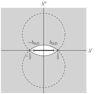
The program of estimating the spectrum of the NP operator goes back to Poincaré [36] as the name suggests, and was recently revisited in [29] with a new perspective. The spectrum of the NP operator also has been studied using complex function theory such as the Beurling-Ahlfors transform and quasi-conformal mapping, for which we refer to [35] (and references therein) where a bound on the essential spectrum of the NP operator for two dimensional domains with corners is obtained. It is proved in [38] that the set $\mathbb{R}\setminus(-1/2,1/2)$ is contained in the resolvent set of the NP operator on $L^{2}_{0}(\partial\Omega)$ for a domain $\Omega$ with the Lipschtz boundary. Its spectrum on $H^{-1/2}$ lies in $(-1/2,1/2]$ (see [18]). Recently the spectral theory of the NP operator has been applied to analysis of cloaking by anomalous localized resonance on the plasmonic structure [2], analysis of high concentration of the gradient [3] [14] [15] [32], and a shape optimization problem [1].

This paper is organized as follows. In section 2 we review symmetrization and spectral properties of the Neumann-Poincaré operator and prove equivalence of norms. In section 3 we deal with the transmission problem in the whole space $\mathbb{R}^{d}$. In section 4 we deal with the boundary value problem and show that the solution exists and is unique, it is bounded in its $H^{1}$-norm uniformly in $k$ away from a closed interval in the negative real axis, and a quantitative estimate is derived which shows that the solution depends Lipschitz continuously on $k$. We then show in section 5 that the boundary perturbation formula when the inclusion is diametrically small is valid uniformly in $k$. The last section is to deal with the case when there are multiple inclusions.

Let $\Gamma(x)$ be the fundamental solution to the Laplacian, i.e.,

where $\omega_{d}$ denotes the area of the unit sphere in $\mathbb{R}^{d}$. Suppose that the inclusion $D$ has a single simply connected component. The single layer potential $\mathcal{S}_{\partial D}[\varphi]$ of a density function $\varphi\in H^{-1/2}(\partial D)$ is defined by

It is well known (see for example [7] [21]) that $\mathcal{S}_{\partial D}[\varphi]$ satisfies the jump relation

where $\frac{\partial}{\partial\nu}$ denotes the outward normal derivative, the subscripts $\pm$ indicate the limit from outside and inside $D$, respectively, and the operator $\mathcal{K}_{\partial D}^{*}$ is defined by

Here $\nu_{x}$ denotes the outward unit normal vector to $\partial D$ at $x$.

The operator $\mathcal{K}_{\partial D}^{*}$ is called the Neumann-Poincaré (NP) operator associated with the domain $D$. If $\partial D$ is Lipschitz continuous, then $\mathcal{K}_{\partial D}^{*}$ is a singular integral operator and known to be bounded on $L^{2}(\partial D)$ (and on $H^{-1/2}(\partial D)$) [20]. Let $H^{-1/2}_{0}(\partial D)$ be the collection of $\varphi\in H^{-1/2}(\partial D)$ with the mean zero, i.e.,

where $\langle\ ,\ \rangle$ is the $H^{-1/2}$-$H^{1/2}$ pairing. For $\varphi,\psi\in H^{-1/2}_{0}(\partial D)$, define

Since $\mathcal{S}_{\partial D}$ maps $H^{-1/2}(\partial D)$ into $H^{1/2}(\partial D)$, the right hand side of (2.6) is well-defined. It is known (see, for example, [2] [15] [23] [29]) that $\langle\ ,\ \rangle_{\mathcal{H}}$ is an inner product on $H^{-1/2}_{0}(\partial D)$ and $\mathcal{K}^{*}_{\partial D}$ is self-adjoint with respect to this inner product, which is a consequence of Plemelj’s symmetrization principle (also known as Calderón’s identity)

Here $\mathcal{K}_{\partial D}$ is the adjoint of $\mathcal{K}^{*}_{\partial D}$ with respect to the usual $L^{2}$-inner product. It is worth mentioning that $\mathcal{K}^{*}_{\partial D}$ is not self-adjoint in the usual inner product unless the domain $D$ is a disk or a ball [31]. Let $\mathcal{H}=\mathcal{H}(\partial D)$ be the space $H^{-1/2}_{0}(\partial D)$ equipped with the inner product $\langle\ ,\ \rangle_{\mathcal{H}}$. We denote the norm associated with $\langle\ ,\ \rangle_{\mathcal{H}}$ by $\|\,\cdot\,\|_{\mathcal{H}}$.

Let us write $\|\varphi\|_{H^{s}(\partial D)}$ as $\|\varphi\|_{s}$ from now on for ease of notation.

In three or higher dimensions, it is proved in [38] that $\mathcal{S}_{\partial D}:L^{2}(\partial D)\to H^{1}(\partial D)$ is invertible. So, $A$ is a Fredholm operator of index zero. Thus one can show by the exactly the same proof as in two dimensions that $A:L^{2}(\partial D)\times\mathbb{C}\to H^{1}(\partial D)\times\mathbb{C}$ is invertible in three dimensions. So we obtain the desired result by the same argument (duality and interpolation). $\Box$

Lemma 2.1 says that for any $f\in H^{1/2}(\partial D)$ and $b\in\mathbb{C}$ there is a unique pair $(\psi,a)\in H^{-1/2}(\partial D)\times\mathbb{C}$ such that $\langle\psi,1\rangle=b$,

and

for some constant $C$. In particular, if we take $b=0$, then $\psi\in H^{-1/2}_{0}(\partial D)$ and (2.10) becomes

So, we obtain the following lemma.

As a consequence we obtain the following theorem.

To prove the opposite inequality, for $f\in H^{1/2}(\partial D)$ choose $\psi\in H^{-1/2}_{0}(\partial D)$ satisfying (2.12) and (2.13). Then we have, by the Cauchy-Schwarz inequality and (2.13),

Since the above inequality holds for all $f\in H^{1/2}(\partial D)$, we obtain

This completes the proof. $\Box$

Since $\mathcal{K}_{\partial D}^{*}$ is self-adjoint on $\mathcal{H}$, its spectrum $\sigma(\mathcal{K}_{\partial D}^{*})$ is real, consists of point and continuous spectra, and is a closed set. Moreover, by the spectral resolution theorem (see [39]) there is a family of projection operators $\mathcal{E}(t)$ on $\mathcal{H}$ (called a resolution of identity) such that

Let $b_{\partial D}$ be the spectral bound of $\mathcal{K}^{*}_{\partial D}$, namely,

It is well-known that for any Lipschitz domain $b_{\partial D}\leq\frac{1}{2}$. In fact, it is proved in [28] that

We obtain the following lemma.

Before completing this section let us make a few remarks on the spectrum of the NP operator. If $\partial D$ is $\mathcal{C}^{1,\alpha}$ for some $\alpha>0$, then $\mathcal{K}^{*}_{\partial D}$ is compact and has only a point spectrum accumulating to $0$. The point spectrum of $\mathcal{K}^{*}_{\partial D}$ is completely known when $D$ is a disk, a ball, or an ellipse (see [23]). For example, if $D$ is an ellipse of the long axis $a$ and short axis $b$, then eigenvalues of $\mathcal{K}^{*}_{\partial D}$ are

See [11] [29]. So, if the eccentricity of the ellipse becomes large, the spectral bound approaches to $1/2$. Other than these examples, the complete spectrum of the NP operator on two discs is obtained in relation to the analysis of gradient concentration [14] [32]. On the other hand, a bound for the essential spectrum has been obtained [35].

The solution $u_{k}$ to (1.6) can be represented as

where $\varphi_{k}\in\mathcal{H}(\partial D)$ is the solution to

where $\lambda=\lambda(k)$ is defined by (1.5). In fact, (3.2) is a consequence of the jump relation (2.3) and transmission conditions on $\partial D$:

Note that the righthand side of (3.2) does not depend on $k$. So, in this case, if $\lambda(k)\notin\sigma(\mathcal{K}_{\partial D}^{*})$, then (3.2) is solvable in $\mathcal{H}$, and hence (1.6) has a solution. This is already interesting since a negative $k$ can satisfy the condition $\lambda(k)\notin\sigma(\mathcal{K}_{\partial D}^{*})$. For example, any $k$ with

satisfies the condition.

We obtain the following solvability result.

To show uniqueness of the solution, assume that $u_{k}^{1}$ and $u_{k}^{2}$ are solutions to (1.6). Let $v=u_{k}^{1}-u_{k}^{2}$. Then $v$ is the solution to (1.6) with $h=0$. So we have

where $k=k^{\prime}+ik^{\prime\prime}$. So, if $k^{\prime}>0$, or if $k^{\prime}\leq 0$ and $k^{\prime\prime}\neq 0$, then

So, $v$ is constant. Since $v(x)\to 0$ as $|x|\to\infty$, we conclude that $v=0$.

Uniqueness for the case $k\leq 0$ (and $\lambda(k)\notin\sigma(\mathcal{K}_{\partial D}^{*})$) can be proved as a limiting case of $k+i\delta$ as $\delta\to 0$. For that we need estimate (3.5) with the constant $C$ independent of $\delta$. So the proof will be presented after establishing uniformity results in the following. $\Box$

For $\epsilon>0$ let

It follows from the spectral resolution (2.18) that

where $\lambda=\lambda(k)$. If $k\in R_{\epsilon}$, then $|\lambda-t|\geq\epsilon$ for all $t\in\sigma(\mathcal{K}_{\partial D}^{*})$, and hence we obtain from (3.7) that

Thus we obtain the following theorem from (3.1).

We also have the following theorem on Lipschitz dependency of the solution on $k$.

In this section we consider the boundary value problem (1.2). We first recall a representation formula for a solution $u$ to (1.2). Suppose that (1.2) admits a solution $u\in H^{1}(\Omega)$. Define the harmonic function $h$ in $\Omega$ by

where the double layer potential $\mathcal{D}_{\partial\Omega}[\varphi]$ is defined by

It is proved in [25] [27] that $u$ is represented as

for some $\varphi\in\mathcal{H}$. In fact, $\varphi$ is given by

and satisfies

where $\lambda=\lambda(k)$ is defined by (1.5).

There is yet another representation for a solution $u$. For $y\in\Omega$ let $N_{y}(x)=N(x,y)$ be the Neumann function on $\Omega$, which is the solution to

References

- [1] H. Ammari, Y.T. Chow, K. Liu J. Zou, Optimal shape design by partial spectral data, SIAM J. Sci. Comput., to appear, arXiv:1310.6098v1.
- [2] H. Ammari, G. Ciraolo, H. Kang, H. Lee G.W. Milton, Spectral theory of a Neumann-Poincaré-type operator and analysis of cloaking due to anomalous localized resonance, Arch. Ration. Mech. An. 208 (2013), 667–692.
- [3] H. Ammari, G. Ciraolo, H. Kang, H. Lee K. Yun, Spectral analysis of the Neumann-Poincaré operator and characterization of the stress concentration in anti-plane elasticity, Arch. Ration. Mech. An. 208 (2013), 275–304.
- [4] H. Ammari, J. Garnier, W. Jing, H. Kang, M. Lim, K. Solna H. Wang, Mathematical and statistical methods for multistatic imaging, Lecture Notes in Math. 2098, Springer, 2013.
- [5] H. Ammari H. Kang, High-order terms in the asymptotic expansions of the steady-state voltage potentials in the presence of conductivity inhomogeneities of small diameter, SIAM J. Math. Anal. 34 (2003), 1152–1166.
- [6] H. Ammari H. Kang, Reconstruction of small inhomogeneities from boundary measurements, Lecture Notes in Mathematics, 1846, Springer-Verlag, Berlin, 2004.
- [7] H. Ammari H. Kang, Polarization and moment tensors, Applied Mathematical Sciences, 162, Springer, New York. 2007.
- [8] H. Ammari H. Kang, Expansion Methods, Handbook of Mathematical Methods of Imaging, 447-499, Springer, 2011.
- [9] H. Ammari, H. Kang, K. Kim H. Lee, Strong convergence of the solutions of the linear elasticity and uniformity of asymptotic expansions in the presence of small inclusions, J. Differ. Equations 254 (2013), 4446–4464.
- [10] H. Ammari, H. Kang, E. Kim M. Lim, Reconstruction of closely spaced small inclusions, SIAM J. Numer. Anal. 42 (2005), 2408–2428.
- [11] H. Ammari, H. Kang H. Lee, A boundary integral method for computing elastic moment tensors for ellipses and ellipsoids, J. Comput. Math. 25 (2007), 2–12.
- [12] H. Ammari, H. Kang, G. Nakamura K. Tanuma, Complete asymptotic expansions of solutions of the system of elastostatics in the presence of an inclusion of small diameter and detection of an inclusion, J. Elasticity 67 (2002), 97–129.
- [13] E. Beretta, E. Francini S. Vessella, ‘Size estimates for the EIT problem with one measurement: the complex case’, Rev. Mat. Iberoamericana 30 (2014), 551-580.
- [14] E. Bonnetier F. Triki, Pointwise bounds on the gradient and the spectrum of the Neumann-Poincaré operator: The case of 2 discs, Contemp. Math. 577 (2012), 79–90.
- [15] E. Bonnetier F. Triki, On the spectrum of Poincaré variational problem for two close-to-touching inclusions in 2D, Arch. Ration. Mech. An. 209 (2013), 541–567.
- [16] M. Brühl, M. Hanke M.S. Vogelius, A direct impedance tomography algorithm for locating small inhomogeneities, Numer. Math. 93 (2003), 635–654.
- [17] Y. Capdeboscq M.S. Vogelius, A general representation formula for boundary voltage perturbations caused by internal conductivity inhomogeneities of low volume fraction, Math. Model. Numer. Anal. 37 (2003) 159–173.
- [18] T. Chang K. Lee, Spectral properties of the layer potentials on Lipschitz domains, Illinois J. Math. 52 (2008), 463–472.
- [19] D. J. Cedio-Fengya, S. Moskow M. S. Vogelius, Identification of conductivity imperfections of small diameter by boundary measurements. Continuous dependence and computational reconstruction, Inverse Problems 14 (1998), 553–595.
- [20] R.R. Coifman, A. McIntosh Y. Meyer, L’intégrale de Cauchy définit un opérateur borné sur pour les courbes lipschitziennes, Ann. Math. 116 (1982), 361–387.
- [21] G. B. Folland, Introduction to partial differential equations, 2nd Ed., Princeton Univ. Press, Princeton, 1995.
- [22] A. Friedman M. Vogelius, Identification of small inhomogeneities of extreme conductivity by boundary measurements: a theorem on continuous dependence, Arch. Ration. Mech. An. 105 (1989), 299–326.
- [23] H. Kang, Layer potential approaches to interface problems, Inverse problems and imaging, Panoramas et Syntheses, Panorama et Synthèsis 44, Societe Mathematique de France, 2015.
- [24] H. Kang, K. Kim, H. Lee, X. Li G.W. Milton, Bounds on the size of an inclusion using the translation method for two-dimensional complex conductivity, SIAM J. Appl. Math. 74 (2014), 939–958.
- [25] H. Kang J.-K. Seo, Layer potential techniques for the inverse conductivity problems, Inverse Problems 12 (1996), 267–278.
- [26] H. Kang J.-K. Seo, Identification of domains with near-extreme conductivity: global stability and error estimates, Inverse Problems 15 (1999), 851–867.
- [27] H. Kang J.-K. Seo, Recent progress in the inverse conductivity problem with single measurement, Inverse problems and related topics (Kobe, 1998), Chapman & Hall/CRC Res. Notes Math. 419, 69–80, 2000.
- [28] O. D. Kellogg, Foundations of potential theory, Dover, New York, 1953 (Reprint from the first edition of Die Grundlehren der Mathematischen Wissenschaften, Band 31, Springer-Verlag, Berlin-New York, 1929).
- [29] D. Khavinson, M. Putinar H. S. Shapiro, Poincaré’s variational problem in potential theory, Arch. Ration. Mech. An. 185 (2007), 143–184.
- [30] S. Kim, J. Lee, J.-K. Seo, E. J. Woo H. Zribi, MultiFrequency trans-admittance scanner: Mathematical framework and feasibility, SIAM J. App. Math. 69 (2008), 22–36.
- [31] M. Lim, Symmetry of a boundary integral operator and a characterization of a ball, Illinois J. Math. 45 (2001), 537–543.
- [32] M. Lim S. Yu, Asymptotics of the solution to the conductivity equation in the presence of adjacent circular inclusions with finite conductivities, J. Math. Anal. Appl. 421 (2015), 131-156.
- [33] E. H. Lockwood, A Book of Curves, Cambridge University Press, 1967.
- [34] H. Nguyen and M. S. Vogelius, A representation formula for the voltage perturbations caused by diametrically small conductivity inhomogeneities. Proof of uniform validity, Ann I H Poincaré-AN 26 (2009), 2283–2315.
- [35] K. Perfekt and M. Putinar, Spectral bounds for the Neumann-Poincaré operator on planar domains with corners, J. Anal. Math. 124 (2014), 39-57.
- [36] H. Poincaré, La méthode de Neumann et le problème de Dirichlet, Acta Math. 20 (1896), 59–142.
- [37] A.E. Thaler and G.W. Milton, Bounds on the volume of an inclusion in a body from a complex conductivity measurement, Commun. Math. Sci. 13 (2015), 863–892.
- [38] G.C. Verchota, Layer potentials and regularity for the Dirichlet problem for Laplace’s equation in Lipschitz domains, J. Funct. Anal. 59 (1984), 572–611.
- [39] K. Yosida, Functional Analysis, 4th Ed., Springer, Berlin, 1974.