跳到论文正文
W Papers独立论文阅读器 arXiv:1406.3811 论文正文 计算阅读时间 · 0%
引用这篇论文根据当前论文元数据生成,正式投稿前建议核对。


License: arXiv.org perpetual non-exclusive license
arXiv:1406.3811v3 [math.OC] 13 Feb 2015

Optimal control of anthracnose using mixed strategies

David Jaures FOTSA MBOGNE Affiliation:  Department of Mathematics and Computer Science
ENSAI, The University of Ngaoundere
Email: mjdavidfotsa@gmail.com
   Christopher THRON Affiliation: 
Texas A&M University, Central Texas
Email:thron@ct.tamus.edu
Abstract

In this paper we propose and study a spatial diffusion model for the control of anthracnose disease in a bounded domain. The model is a generalization of the one previously developed in [14]. We use the model to simulate two different types of control strategies against anthracnose disease. Strategies that employ chemical fungicides are modeled using a continuous control function; while strategies that rely on cultivational practices (such as pruning and removal of mummified fruits) are modeled with a control function which is discrete in time (though not in space). Under weak smoothness conditions on parameters we demonstrate the well-posedness of the model by verifying existence and uniqueness of the solution for given initial conditions. We also show that the set [0,1]\left[0,1\right] is positively invariant. We first study control by pulse strategy only, then analyze the simultaneous use of continuous and pulse strategies. In each case we specify a cost functional to be minimized, and we demonstrate the existence of optimal control strategies that can be evaluated numerically using the gradient method presented in [1]. We discuss the results of numerical simulations both for a spatially-averaged version of the model and for the full model.

KeyWords— Anthracnose modelling, nonlinear systems, impulsive PDE, optimal control.

AMS Classification— 49J20, 49J15, 92D30, 92D40.

I Introduction

Anthracnose is a phytopathology which attacks several commercial tropical crops such as coffee. The Anthracnose of coffee is known under the name coffee berry disease (CBD) and its pathogen is the Colletotrichum kahawae, an ascomycete fungus. The literature on Anthracnose pathosystem is extensive [4, 5, 7, 16, 18, 23, 28]. There have been several attempts to model the spread of CBD and to identify efficient control strategies [10, 11, 13, 17, 18, 19, 20, 21, 28]. Possible control methods include genetic methods [3, 4, 5, 15, 27], biological control [12], chemical control [5, 22, 24] and cultivational practices [5, 19, 20, 21, 28]. Chemical methods appear to be the most effective, but present ecological risks. Moreover, inadequate application of chemical treatments can induce resistance in the pathogen [26].

A dynamical spatial model of anthracnose infection that includes chemical control was proposed and analysed in [14]; this paper also showed how to optimize the use of the chemical control with respect to a given cost functional. The disease dynamics were represented by an inhibition rate that satisfies a reaction-diffusion partial differential equation with coefficients that depend on space and time. The present paper adds to the above model the possibility of a pulse control strategy that represents cultivational practices such as pruning old, infected twigs and removing mummified fruits. Such actions are commonly performed at discrete times at regular intervals. An additional enhancement to the model results from our relaxing the regularity conditions on the model parameters that were imposed in [14]. The enhanced model is able to take into account the fact that in realistic situations the application of antifungal compounds is typically not continuous in time (although the action of these compounds once applied is continuous).

The remainder of the paper has the following structure. In section II, we present the system model and explain the significance of the model parameters. In section III we establish the well-posedness of the model (4)−(7)\left(\ref{ModelPulse1}\right)-\left(\ref{ModelPulse4}\right) (under certain conditions) and its spatially-averaged version. Section IV proves existence of an optimal control strategy based only on the pulse strategy, for both the spatially-averaged model and the general model. Some properties of the optimal control strategy are proven, and an algorithm for finding the optimal pulse strategy is given, which applies both spatially-averaged and general models. Section Vproves the existence of an optimal control strategy using simultaneously pulse and continuous strategies, for both the spatially-averaged and the general model. Some extremal properties of these strategies are also established. In Section VI we present system simulations of both the spatially-averaged and general models that demonstrate properties of the optimal pulse-only control. Finally, in section VII we summarize our conclusions.

II System model

The model of anthracnose infection discussed in [14] expressed the disease dynamics in terms of an inhibition rate θ\theta that satisfies the following equations:

∂tθ=α(t,x,θ)(1−θ/(1−σu(t,x)))+div(A(t,x,θ)∇θ)\displaystyle\partial_{t}\theta=\alpha\left(t,x,\theta\right)\left(1-\theta/\left(1-\sigma u\left(t,x\right)\right)\right)+\operatorname{div}\left(A\left(t,x,\theta\right)\nabla\theta\right)
 on ​(t,x)∈ℝ+∗×Ω;\displaystyle\qquad\quad\text{ on }(t,x)\in\mathbb{R}_{+}^{\ast}\times\Omega; (1)
⟨A(t,x,θ)∇θ(t,x),n(x)⟩=0, on ℝ+∗×∂Ω;\displaystyle\left\langle A\left(t,x,\theta\right)\nabla\theta\left(t,x\right),n\left(x\right)\right\rangle=0,\text{ on }\mathbb{R}_{+}^{\ast}\times\partial\Omega; (2)
θ⁡(0,x)=ρ⁡(x),x∈Ω¯⊆ℝ3,\displaystyle\theta\left(0,x\right)=\rho\left(x\right),x\in\overline{\Omega}\subseteq\mathbb{R}^{3}, (3)

where

α⁡(t,x,θ)\alpha(t,x,\theta) is a positive real-valued function defined on (t,x)∈ℝ+∗×Ω(t,x)\in\mathbb{R}_{+}^{\ast}\times\Omega;

σ\sigma is a real parameter satisfying 0≤σ≤10\leq\sigma\leq 1;

u⁡(x,t)u(x,t) is a real-valued function with 0≤u⁡(x,t)≤10\leq u(x,t)\leq 1, defined on the same domain as α\alpha;

A⁡(t,x,θ)A(t,x,\theta) is a 3×33\times 3 matrix function which is positive definite for all t,x,θt,x,\theta, defined on the same domain as α\alpha;

Ω\Omega is an open, bounded subset of ℝ3\mathbb{R}^{3};

∂Ω\partial\Omega is the boundary of Ω\Omega, which is assumed to satisfy ∂Ω∈H1​(ℝ2,ℝ)\partial\Omega\in H^{1}\left(\mathbb{R}^{2};\mathbb{R}\right);

n⁡(x)n\left(x\right) denotes the normal vector to the boundary at x∈∂Ωx\in\partial\Omega;

ρ⁡(x)\rho(x) is a real-valued function satisfying 0≤ρ⁡(x)≤10\leq\rho(x)\leq 1 for x∈Ω¯x\in\overline{\Omega}.

The various terms in the model equations (1)−(3)(\ref{ModelOrig1})-(\ref{ModelOrig3}) have practical interpretations as follows. (See reference [14] for a more detailed description.) The function α\alpha represents the inhibition pressure, which depends on climatic and environmental conditions [10, 11, 13]. It is appropriate to model α\alpha as an almost-periodic function, taking into account yearly seasonal changes. The term div(A∇θ)\operatorname{div}\left(A\nabla\theta\right) accounts for the (possibly anisotropic) diffusive spatial spreading of inhibition rate in the open domain Ω⊂ℝ3\Omega\subset\mathbb{R}^{3}, where the matrix AA contains the space- and time-dependent diffusion coefficients. The boundary condition ⟨A∇θ,n⟩=0\left\langle A\nabla\theta,n\right\rangle=0 guarantees that there is no net flux of inhibition rate between Ω\Omega and its exterior. The function u⁡(x,t)u(x,t) expresses the influence of chemical control (that is, the application of fungicides) on the inhibition rate. 1−σ1-\sigma is the inhibition rate corresponding to epidermis penetration. Once the epidermis has been penetrated, the inhibition rate cannot fall below this value, even under maximum control effort.

In the current paper, we propose the following modified model, that includes the possibility of impulsive control:

∂tθ=α(t,x)(1−θ/(1−σu(t,x)))+div(A(t,x)∇θ),\displaystyle\partial_{t}\theta=\alpha\left(t,x\right)\left(1-\theta/\left(1-\sigma u\left(t,x\right)\right)\right)+\operatorname{div}\left(A\left(t,x\right)\nabla\theta\right),
(t,x)∈(ℝ+∗∖{τi}i∈ℕ)×Ω;\displaystyle\qquad\quad(t,x)\in\left(\mathbb{R}_{+}^{\ast}\setminus\left\{\tau_{i}\right\}_{i\in\mathbb{N}}\right)\times\Omega; (4)
θ(τi+,x)=vi(x)θ(τi,x), i∈ℕ∗,x∈Ω;\displaystyle\theta\left(\tau_{i}^{+},x\right)=v_{i}\left(x\right)\theta\left(\tau_{i},x\right),\text{ }i\in\mathbb{N}^{\ast},x\in\Omega; (5)
⟨A(t,x)∇θ(t,x),n(x)⟩=0,\displaystyle\left\langle A\left(t,x\right)\nabla\theta\left(t,x\right),n\left(x\right)\right\rangle=0,
(t,x)∈(ℝ+∗∖{τi}i∈ℕ)×∂Ω;\displaystyle\qquad\quad(t,x)\in\left(\mathbb{R}_{+}^{\ast}\setminus\left\{\tau_{i}\right\}_{i\in\mathbb{N}}\right)\times\partial\Omega; (6)
θ⁡(0,x)=ρ⁡(x)≥0,x∈Ω¯⊆ℝ3,\displaystyle\theta\left(0,x\right)=\rho\left(x\right)\geq 0,x\in\overline{\Omega}\subseteq\mathbb{R}^{3}, (7)

where α\alpha, uu, σ\sigma, AA, Ω\Omega, n⁡(x)n\left(x\right), and ρ⁡(x)\rho(x) are as above (except that α\alpha and AA no longer depend on θ\theta) and

(tk)k∈ℕ\left(t_{k}\right)_{k\in\mathbb{N}} is an increasing sequence of nonnegative reals such that limk→∞​tk=∞\underset{k\rightarrow\infty}{\lim}t_{k}=\infty;

τ0=t0=0\tau_{0}=t_{0}=0;

τi=inf{tk>τi−1;k>0 and ‖θ(tk,.)‖L2​(Ω)≥σ∗|Ω|}\tau_{i}=\inf\left\{t_{k}>\tau_{i-1};k>0\text{ and }\left\|\theta\left(t_{k},.\right)\right\|_{L^{2}\left(\Omega\right)}\geq\sigma^{\ast}\left|\Omega\right|\right\}, where |Ω|\left|\Omega\right| denotes the volume ∫Ω𝑑x{\displaystyle\int\nolimits_{\Omega}}dx;

σ∗∈ℝ+\sigma^{\ast}\in\mathbb{R}^{+} is a threshold value such that the inhibition rate is not measurable under it and is observable for values greater than σ∗\sigma^{\ast};

vi​(x),i=1,2,3,…v_{i}(x),i=1,2,3,\ldots is a [0,1][0,1]-valued function defined on x∈Ωx\in\Omega.

In (4)−(7)(\ref{ModelPulse1})-(\ref{ModelPulse4}), the inhibition rate θ\theta is assumed to be left continuous with respect to time: θ(t,.)=θ(t−,x)\theta\left(t,.\right)=\theta\left(t^{-},x\right), where θ⁡(t−,x)\theta\left(t^{-},x\right) denotes lims→t,s<t​θ​(s,x)\underset{s\rightarrow t,s<t}{\lim}\theta\left(s,x\right). (We shall also use the notation θ⁡(t+,x)\theta\left(t^{+},x\right) to denote lims→t,s>t​θ​(s,x).\underset{s\rightarrow t,s>t}{\lim}\theta\left(s,x\right).)

Cultivational practices are included in the model (4)−(7)(\ref{ModelPulse1})-(\ref{ModelPulse4}) as follows. The sequence (tk)k∈ℕ\left(t_{k}\right)_{k\in\mathbb{N}} represents times at which cultivational interventions are possible. For example, in coffee cultivation it would be reasonable to take the tk′​st_{k}^{\prime}s as regularly spaced with an interval of one week. The intervals between intervention times reflect the fact that continuous exertion of cultivational interventions such as pruning is neither practical nor efficient. At each potential intervention time tkt_{k}, intervention only takes place if the infection is sufficiently serious, as determined by the threshold condition ‖θ(tk,.)‖H1​(Ω)≥σ∗\left\|\theta(t_{k},.)\right\|_{H^{1}(\Omega)}\geq\sigma^{\ast}. The degree of intervention at time τi\tau_{i} at each point x∈Ωx\in\Omega is given by vi​(x)v_{i}(x): vi​(x)=1v_{i}(x)=1 corresponds to no change in the inhibition rate at xx, while vi​(x)=0v_{i}(x)=0 reduces the inhibition rate θ⁡(x)\theta(x) to 00.

III Well-posedness of the model

In this section we verify that the model (4)−(7)(\ref{ModelPulse1})-(\ref{ModelPulse4}) is well-posed (under certain conditions) and that the inhibition rate θ⁡(t,x)\theta(t,x) always remains between 00 and 11. We first establish well-posedness of a spatially-averaged version of the model, and then use similar techniques to prove well-posedness of the spatially-dependent model.

III-A Well-posedness of spatially-averaged model

A spatially-averaged version of the model (4)−(7)(\ref{ModelPulse1})-(\ref{ModelPulse4}) may be obtained by taking spatial averages of the equations. The averaged model is much simpler to work with than the general model; however, the same tools used to prove well-posedness for the averaged model can be generalized to apply to the general model.

Define

Θ⁡(t)≡1|Ω|​∫Ωθ⁡(t,x)​𝑑x.\Theta\left(t\right)\equiv\frac{1}{\left|\Omega\right|}{\displaystyle\int\nolimits_{\Omega}}\theta\left(t,x\right)dx. (8)

If we suppose that α,\alpha, uu and viv_{i} are functions of tt only and not of xx, then Θ⁡(t)\Theta(t) satisfies the following impulsive differential equation:

dt​Θ=α⁡(t)​(1−Θ/(1−σ​u​(t))), on ​ℝ+∗∖(τi)i∈ℕ;\displaystyle d_{t}\Theta=\alpha\left(t\right)\left(1-\Theta/\left(1-\sigma u\left(t\right)\right)\right),\text{ on }\mathbb{R}_{+}^{\ast}\setminus\left(\tau_{i}\right)_{i\in\mathbb{N}}; (9)
Θ⁡(τi+)=vi​Θ​(τi),i∈ℕ∗,\displaystyle\Theta\left(\tau_{i}^{+}\right)=v_{i}\Theta\left(\tau_{i}\right),~i\in\mathbb{N}^{\ast}, (10)
Θ⁡(0)=Θ0∈[0,1],\displaystyle\Theta\left(0\right)=\Theta_{0}\in\left[0,1\right], (11)

where

τ0=t0=0;\displaystyle\tau_{0}=t_{0}=0; (12)
τi=inf{tk>τi−1;k>0, Θ(tk)≥σ∗}.\displaystyle\tau_{i}=\inf\left\{t_{k}>\tau_{i-1};k>0,\text{ }\Theta\left(t_{k}\right)\geq\sigma^{\ast}\right\}. (13)

Note that the divergence term in (4) vanishes in the averaged model, due to the no-flux boundary conditions (6).

A solution of (9)−(11)\left(\ref{ModelPulse1IDE}\right)-\left(\ref{ModelPulse3IDE}\right) is a piecewise absolutely continuous real-valued function that satisfies the following equation in each interval ]τk,τk+1]\left]\tau_{k},\tau_{k+1}\right]:

Θ⁡(t)=Θ⁡(τk+)+∫τktα⁡(s)​(1−Θ⁡(s)/(1−σ​u​(s)))​𝑑s.\Theta\left(t\right)=\Theta\left(\tau_{k}^{+}\right)+{\displaystyle\int\nolimits_{\tau_{k}}^{t}}\alpha\left(s\right)\left(1-\Theta\left(s\right)/\left(1-\sigma u\left(s\right)\right)\right)ds. (14)

We impose the following conditions on α\alpha and uu to ensure the solution’s existence and uniqueness:

(H1): α∈Ll​o​c∞​(ℝ+,ℝ+)~~\alpha\in L_{loc}^{\infty}\left(\mathbb{R}_{+};\mathbb{R}_{+}\right).

(H2): u∈L∞​(ℝ+,[0,1])~~u\in L^{\infty}\left(\mathbb{R}_{+};\left[0,1\right]\right).

Proposition 1

If Θ\Theta is a maximal solution of (9)−(11)\left(\ref{ModelPulse1IDE}\right)-\left(\ref{ModelPulse3IDE}\right), then Θ\Theta is [0,1]−\left[0,1\right]-valued.

Proof:

Let Θ\Theta be a solution of (9)−(11)\left(\ref{ModelPulse1IDE}\right)-\left(\ref{ModelPulse3IDE}\right). Since vi∈[0,1]v_{i}\in\left[0,1\right] it suffices to establish that the restriction of Θ\Theta on ]t0,t1]\left]t_{0},t_{1}\right] is [0,1]−\left[0,1\right]-valued. Let f=max⁡{0,−Θ}f=\max\left\{0,-\Theta\right\} and g=max⁡{0,Θ−1}g=\max\left\{0,\Theta-1\right\}.

We first prove that Θ≥0\Theta\geq 0. Let U⊂]t0,t1]U\subset\left]t_{0},t_{1}\right] be the set where ff is positive. Since ff is continuous, it follows that UU is open in ]t0,t1]\left]t_{0},t_{1}\right]. Suppose that UU is nonempty; then UU is the disjoint union of open subintervals of ]t0,t1]\left]t_{0},t_{1}\right]. Let U′≠∅U^{\prime}\neq\emptyset be one of these intervals. Then from (14) and the definition of ff, for t∈U′t\in U^{\prime} we have

f⁡(t)\displaystyle f\left(t\right) =∫infU′t−α(s)(1+f(s)/(1−σu(s)))ds\displaystyle={\displaystyle\int\nolimits_{\inf U^{\prime}}^{t}}-\alpha\left(s\right)\left(1+f\left(s\right)/\left(1-\sigma u\left(s\right)\right)\right)ds
≤0.\displaystyle\leq 0.

But we know f⁡(t)>0f(t)>0, since t∈U′t\in U^{\prime}; this contradiction implies that UU is empty. It follows that f=0f=0 on ]t0,t1]\left]t_{0},t_{1}\right], which implies that Θ≥0\Theta\geq 0 on ]t0,t1]\left]t_{0},t_{1}\right].

To prove that Θ≤1\Theta\leq 1 on ]t0,t1]\left]t_{0},t_{1}\right], we may use an almost identical argument, with g⁡(x)g(x) replacing f⁡(x)f(x). ∎

Proposition 2

The problem (9)−(11)\left(\ref{ModelPulse1IDE}\right)-\left(\ref{ModelPulse3IDE}\right) has a unique global solution.

Proof:

For existence, it suffices to establish existence of a local solution and use Proposition 1 to conclude the result based on Theorem 5.7 of [8]. It also suffices to restrict ourselves to the set [t0+,t1]\left[t_{0}^{+},t_{1}\right]. The function (t,x)∈[t0+,t1]×[0,1]↦α⁡(t)​(1−x/(1−σ​u​(t)))\left(t,x\right)\in\left[t_{0}^{+},t_{1}\right]\times\left[0,1\right]\mapsto\alpha\left(t\right)\left(1-x/\left(1-\sigma u\left(t\right)\right)\right) is integrable with respect to tt, Lipschitz continuous with respect to xx, and upper bounded by α\alpha which is also integrable with respect to tt. Then by the Carathéodory theorem (see [9]) there is a local [0,1]−\left[0,1\right]-valued solution.

We now prove uniqueness of the solution. Given that xx and yy are solutions on [t0+,t1]\left[t_{0}^{+},t_{1}\right], we have that

|x⁡(t)−y⁡(t)|\displaystyle\left|x\left(t\right)-y\left(t\right)\right| ≤|x⁡(t0+)−y⁡(t0+)|\displaystyle\leq\left|x\left(t_{0}^{+}\right)-y\left(t_{0}^{+}\right)\right|
+∫t0tα(s)|y(s)−x(s)|/(1−σu(s))ds.\displaystyle+{\displaystyle\int\nolimits_{t_{0}}^{t}}\alpha\left(s\right)\left|y\left(s\right)-x\left(s\right)\right|/\left(1-\sigma u\left(s\right)\right)ds.

Using the Gronwall lemma, we get

|x⁡(t)−y⁡(t)|\displaystyle\left|x\left(t\right)-y\left(t\right)\right| ≤|x⁡(t0+)−y⁡(t0+)|\displaystyle\leq\left|x\left(t_{0}^{+}\right)-y\left(t_{0}^{+}\right)\right|
×exp⁡(∫t0tα⁡(s)/(1−σ​u​(s))​𝑑s)\displaystyle\times\exp\left({\displaystyle\int\nolimits_{t_{0}}^{t}}\alpha\left(s\right)/\left(1-\sigma u\left(s\right)\right)ds\right)

and more generally if t∈t\in [tk+,tk+1]\left[t_{k}^{+},t_{k+1}\right]

|x⁡(t)−y⁡(t)|\displaystyle\left|x\left(t\right)-y\left(t\right)\right| ≤(∏i=0kvi)​|x⁡(t0)−y⁡(t0)|\displaystyle\leq\left({\displaystyle\prod\nolimits_{i=0}^{k}}v_{i}\right)\left|x\left(t_{0}\right)-y\left(t_{0}\right)\right|
×exp⁡(∫t0tα⁡(s)/(1−σ​u​(s))​𝑑s)\displaystyle\times\exp\left({\displaystyle\int\nolimits_{t_{0}}^{t}}\alpha\left(s\right)/\left(1-\sigma u\left(s\right)\right)ds\right) (15)

It follows that the solution is unique and depends continuously on initial conditions. ∎

It is important to notice that (15) implies that the solution of (9)−(11)\left(\ref{ModelPulse1IDE}\right)-\left(\ref{ModelPulse3IDE}\right) is continuous with respect to control strategies uu and (vi)\left(v_{i}\right).

III-B Well-posedness of the general model

A solution θ\theta of (4)−(7)\left(\ref{ModelPulse1}\right)-\left(\ref{ModelPulse4}\right) is a piecewise absolutely continuous function of time, such that ∀t≥0\forall t\geq 0 the function θ(t,.)∈H2(Ω;ℝ)\theta\left(t,.\right)\in H^{2}(\Omega;\mathbb{R}) and satisfies

θ⁡(t,x)\displaystyle\theta\left(t,x\right) =θ⁡(τk+,x)\displaystyle=\theta\left(\tau_{k}^{+},x\right)
+∫τktα(s,x)(1−θ(s,x)/(1−σu(s,x)))ds\displaystyle+{\displaystyle\int\nolimits_{\tau_{k}}^{t}}\alpha\left(s,x\right)\left(1-\theta\left(s,x\right)/\left(1-\sigma u\left(s,x\right)\right)\right)ds
+∫τktdiv(A(s,x)∇θ(s,x))ds;\displaystyle+{\displaystyle\int\nolimits_{\tau_{k}}^{t}}\operatorname{div}\left(A\left(s,x\right)\nabla\theta\left(s,x\right)\right)ds; (16)
⟨A(t,x)∇θ(t,x),n(x)⟩=0\displaystyle\left\langle A\left(t,x\right)\nabla\theta\left(t,x\right),n\left(x\right)\right\rangle=0
 on ​(ℝ+∗∖(τi)i∈ℕ)×∂Ω;\displaystyle\qquad\qquad\qquad\qquad\qquad\text{ on }\left(\mathbb{R}_{+}^{\ast}\setminus\left(\tau_{i}\right)_{i\in\mathbb{N}}\right)\times\partial\Omega; (17)

for all t∈]τk,τk+1]t\in]\tau_{k},\tau_{k+1}] and ∀x∈Ω\forall x\in\Omega. We also have

θ(0,x)=ρ(x)∈[0,1], ∀x∈Ω¯⊆ℝ3.\theta\left(0,x\right)=\rho\left(x\right)\in\left[0,1\right],\text{ }\forall x\in\overline{\Omega}\subseteq\mathbb{R}^{3}. (18)

We further define a weak solution θ\theta of (4)−(7)\left(\ref{ModelPulse1}\right)-\left(\ref{ModelPulse4}\right) to be a piecewise absolutely continuous function with respect to time which satisfies (18) and ∀t≥0,\forall t\geq 0, the function θ(t,.)∈H1(Ω;ℝ)\theta\left(t,.\right)\in H^{1}(\Omega;\mathbb{R}) satisfies (17) and the following “weak” form of (16):

∫Ωθ⁡(t,x)​ψ​(t,x)​𝑑x\displaystyle{\displaystyle\int\nolimits_{\Omega}}\theta\left(t,x\right)\psi\left(t,x\right)dx
=∫Ωθ⁡(τk+,x)​ψ​(τk+,x)​𝑑x\displaystyle={\displaystyle\int\nolimits_{\Omega}}\theta\left(\tau_{k}^{+},x\right)\psi\left(\tau_{k}^{+},x\right)dx
−∫Ω∫τkt⟨A(s,x)∇θ(s,x),∇ψ(s,x)⟩ds\displaystyle-{\displaystyle\int\nolimits_{\Omega}}{\displaystyle\int\nolimits_{\tau_{k}}^{t}}\left\langle A\left(s,x\right)\nabla\theta\left(s,x\right),\nabla\psi\left(s,x\right)\right\rangle ds
+∫Ω∫τktα(s,x)ψ(s,x)(1−θ(s,x)/(1−σu(s,x)))dsdx,\displaystyle+{\displaystyle\int\nolimits_{\Omega}}{\displaystyle\int\nolimits_{\tau_{k}}^{t}}\alpha\left(s,x\right)\psi\left(s,x\right)\left(1-\theta\left(s,x\right)/\left(1-\sigma u\left(s,x\right)\right)\right)ds\,dx,

where t∈]τk,τk+1]t\in]\tau_{k},\tau_{k+1}] and ψ∈H1​(Ω,ℝ)\psi\in H^{1}\left(\Omega;\mathbb{R}\right). We make the following additional assumptions in order to guarantee existence and uniqueness of the weak solution:

(H3): α∈Ll​o​c∞​(ℝ+,L∞​(Ω,ℝ+))\alpha\in L_{loc}^{\infty}\left(\mathbb{R}_{+};L^{\infty}\left(\Omega;\mathbb{R}_{+}\right)\right);

(H4): ∀i,j∈{1,2,3},\forall i,j\in\left\{1,2,3\right\}, ai​j∈Ll​o​c∞​(ℝ+,W1,∞​(Ω,ℝ))a_{ij}\in L_{loc}^{\infty}\left(\mathbb{R}_{+};W^{1,\infty}\left(\Omega;\mathbb{R}\right)\right);

(H5): ∃δ∈ℝ+∗\exists\delta\in\mathbb{R}_{+}^{\ast} such that ∀t∈ℝ+,∀w∈H1​(Ω,ℝ),\forall t\in\mathbb{R}_{+},\forall w\in H^{1}\left(\Omega;\mathbb{R}\right),

∫Ω⟨A(t,x)∇w(x),∇w(x)⟩dx≥δ∫Ω⟨∇w(x),∇w(x)⟩dx;{\displaystyle\int\nolimits_{\Omega}}\left\langle A\left(t,x\right)\nabla w\left(x\right),\nabla w\left(x\right)\right\rangle dx\geq\delta{\displaystyle\int\nolimits_{\Omega}}\left\langle\nabla w\left(x\right),\nabla w\left(x\right)\right\rangle dx;

(H6): u∈L∞​(ℝ+,L∞​(Ω,[0,1]))u\in L^{\infty}\left(\mathbb{R}_{+};L^{\infty}\left(\Omega;\left[0,1\right]\right)\right);

(H7): ∀i∈ℕ,vi∈L∞​(Ω,[0,1])\forall i\in\mathbb{N},v_{i}\in L^{\infty}\left(\Omega;\left[0,1\right]\right).

As preliminary to proving existence and uniqueness of weak solutions, we first establish the boundedness of solutions. The proof is similar to that of Proposition 1.

Proposition 3

If θ\theta is a maximal solution of (4)−(7)\left(\ref{ModelPulse1}\right)-\left(\ref{ModelPulse4}\right) then θ\theta is [0,1]\left[0,1\right]-valued.

Proof:

Let θ\theta be a solution of (4)−(7)\left(\ref{ModelPulse1}\right)-\left(\ref{ModelPulse4}\right). Since vi∈L∞​(Ω,[0,1])v_{i}\in L^{\infty}\left(\Omega;\left[0,1\right]\right) it suffices to establish the result for the restriction of θ\theta on ]t0,t1]\left]t_{0},t_{1}\right]. Let f=max⁡{0,−θ}f=\max\left\{0,-\theta\right\} and g=max⁡{0,θ−1}g=\max\left\{0,\theta-1\right\}.

We first prove that θ≥0\theta\geq 0. Let 𝒰⊂]t0,t1]×Ω\mathcal{U}\subset\left]t_{0},t_{1}\right]\times\Omega be the set where ff is positive. Let Ωt=({t}×Ω)∩𝒰\Omega_{t}=(\{t\}\times\Omega)\cap\mathcal{U}, and let U={t|Ωt≠∅}U=\{t\,|\,\Omega_{t}\neq\emptyset\}. As in the proof of Proposition 1, we may choose an open subinterval U′⊂UU^{\prime}\subset U which is a connected component of UU. For almost every time t∈U′t\in U^{\prime}, the function f(t,.)∈H1(Ω,ℝ)f\left(t,.\right)\in H^{1}\left(\Omega,\mathbb{R}\right) and

12∂t‖f(t,.)‖L2​(Ω,ℝ)2\displaystyle\frac{1}{2}\partial_{t}\left\|f\left(t,.\right)\right\|_{L^{2}\left(\Omega;\mathbb{R}\right)}^{2}
=12​∂t∫Ω2f2​(t,x)​𝑑x\displaystyle=\frac{1}{2}\partial_{t}{\displaystyle\int\nolimits_{\Omega_{2}}}f^{2}\left(t,x\right)dx
=∫Ωf⁡(t,x)​∂tf⁡(t,x)​𝑑x\displaystyle={\displaystyle\int\nolimits_{\Omega}}f\left(t,x\right)\partial_{t}f\left(t,x\right)dx
=−∫Ωα(t,x)f(t,x)dx\displaystyle=-{\displaystyle\int\nolimits_{\Omega}}\alpha\left(t,x\right)f\left(t,x\right)dx
+∫Ωdiv(A(t,x)∇f(t,x))f(t,x)dx\displaystyle+{\displaystyle\int\nolimits_{\Omega}}\operatorname{div}\left(A\left(t,x\right)\nabla f\left(t,x\right)\right)f\left(t,x\right)dx
−∫Ωα(t,x)f2(t,x)/(1−σu(t,x))dx\displaystyle-{\displaystyle\int\nolimits_{\Omega}}\alpha\left(t,x\right)f^{2}\left(t,x\right)/\left(1-\sigma u\left(t,x\right)\right)dx
=−∫Ωα(t,x)f(t,x)dx\displaystyle=-{\displaystyle\int\nolimits_{\Omega}}\alpha\left(t,x\right)f\left(t,x\right)dx
−∫Ω⟨A(t,x)∇f(t,x),∇f(t,x)⟩dx\displaystyle-{\displaystyle\int\nolimits_{\Omega}}\left\langle A\left(t,x\right)\nabla f\left(t,x\right),\nabla f\left(t,x\right)\right\rangle dx
−∫Ωα(t,x)f2(t,x)/(1−σu(t,x))dx\displaystyle-{\displaystyle\int\nolimits_{\Omega}}\alpha\left(t,x\right)f^{2}\left(t,x\right)/\left(1-\sigma u\left(t,x\right)\right)dx
≤0.\displaystyle\leq 0.

Since ‖f(inf(U′),.)‖L2​(Ω,ℝ)=0\left\|f(\inf(U^{\prime}),.)\right\|_{L^{2}(\Omega;\mathbb{R})}=0, it follows that ‖f(t,.)‖L2​(Ω,ℝ)=0\left\|f(t,.)\right\|_{L^{2}(\Omega;\mathbb{R})}=0 for all t∈U′t\in U^{\prime}, which implies f≡0f\equiv 0 in U′×ΩU^{\prime}\times\Omega. It follows immediately that f≡0f\equiv 0 in U×ΩU\times\Omega, so that θ≥0\theta\geq 0 on ]t0,t1]\left]t_{0},t_{1}\right].

A similar computation to the above can be used to show that g≡0g\equiv 0 in U×ΩU\times\Omega, from which θ≤1\theta\leq 1 follows immediately.

∎

From assumptions (H4)-(H5), it follows that the following problem has a unique solution in H1​(Ω)H^{1}\left(\Omega\right) for an arbitrary but fixed time t>0t>0.

{div(A(t,x)∇w(x))=f(x), ∀x∈Ω⟨A(t,x)∇w(x),n(x)⟩=0, ∀x∈∂Ω\left\{\begin{array}[c]{l}\operatorname{div}\left(A\left(t,x\right)\nabla w\left(x\right)\right)=f\left(x\right),\text{ }\forall x\in\Omega\\ \left\langle A\left(t,x\right)\nabla w\left(x\right),n\left(x\right)\right\rangle=0,\text{ }\forall x\in\partial\Omega\end{array}\right.

where f∈L2​(Ω)f\in L^{2}\left(\Omega\right). Theorems 3.6.1 and 3.6.2 of [2] imply that there is a complete orthonormal system {φn(t,.)}n∈ℕ⊂L2(Ω)\left\{\varphi_{n}\left(t,.\right)\right\}_{n\in\mathbb{N}}\subset L^{2}\left(\Omega\right) of eigenfunctions and eigenvalues {λn​(t)}\left\{\lambda_{n}\left(t\right)\right\} such that ∀n∈ℕ,\forall n\in\mathbb{N},

{div(A(t,x)∇φn(t,x))=λn(t)φn(t,x), ∀x∈Ω⟨A(t,x)∇φn(t,x),n(x)⟩=0, ∀x∈∂Ω\left\{\begin{array}[c]{l}\operatorname{div}\left(A\left(t,x\right)\nabla\varphi_{n}\left(t,x\right)\right)=\lambda_{n}\left(t\right)\varphi_{n}\left(t,x\right),\text{ }\forall x\in\Omega\\ \left\langle A\left(t,x\right)\nabla\varphi_{n}\left(t,x\right),n\left(x\right)\right\rangle=0,\text{ }\forall x\in\partial\Omega\end{array}\right.

Moreover, the sequence (φn(t,.))n∈ℕ\left(\varphi_{n}\left(t,.\right)\right)_{n\in\mathbb{N}} is H1​(Ω)−H^{1}\left(\Omega\right)-valued, and if ∂Ω\partial\Omega is of class C2C^{2} then (φn(t,.))n∈ℕ\left(\varphi_{n}\left(t,.\right)\right)_{n\in\mathbb{N}} is H2​(Ω)−H^{2}\left(\Omega\right)-valued.

Now we make the following assumption

(H8): The sequence (φn)\left(\varphi_{n}\right) is independent of time (that is, φn(t,.)=φn(.),\varphi_{n}\left(t,.\right)=\varphi_{n}\left(.\right), ∀t>0\forall t>0).

In particular, (H8) holds if A(t,.)A\left(t,.\right) has the form μ(t)B(.)\mu\left(t\right)B\left(.\right) with μ⁡(t)∈ℝ\mu\left(t\right)\in\mathbb{R}, ∀t≥0\forall t\geq 0. In the special case where A(t,.)=μ(t)IA\left(t,.\right)=\mu\left(t\right)I (II is the 3×33\times 3 identity matrix), we have div(A(t,.)∇w)=μ(t)Δw\operatorname{div}\left(A\left(t,.\right)\nabla w\right)=\mu(t)\Delta w.

When (H8) is satisfied, a weak solution θ\theta of (9)−(11)\left(\ref{ModelPulse1IDE}\right)-\left(\ref{ModelPulse3IDE}\right) can be written as ∑n=0∞θn​φn{\displaystyle\sum\nolimits_{n=0}^{\infty}}\theta_{n}\varphi_{n}, where each θn\theta_{n} is an absolutely continuous function of time that for t∈]τk,τk+1],t\in\left]\tau_{k},\tau_{k+1}\right], satisfies

θn​(t)=∑m=0∞θm​∫Ωφm​(x)​φn​(x)​𝑑x\displaystyle\theta_{n}\left(t\right)={\displaystyle\sum\nolimits_{m=0}^{\infty}}\theta_{m}{\displaystyle\int\nolimits_{\Omega}}\varphi_{m}\left(x\right)\varphi_{n}\left(x\right)dx (19)
=θn​(τk+)+∫τktλn​(s)​θn​(s)​𝑑s\displaystyle=\theta_{n}\left(\tau_{k}^{+}\right)+{\displaystyle\int\nolimits_{\tau_{k}}^{t}}\lambda_{n}\left(s\right)\theta_{n}\left(s\right)ds
−∫τkt∫Ωα(s,x)φn(x)/(1−σu(s,x))\displaystyle-{\displaystyle\int\nolimits_{\tau_{k}}^{t}}{\displaystyle\int\nolimits_{\Omega}}\alpha\left(s,x\right)\varphi_{n}\left(x\right)/\left(1-\sigma u\left(s,x\right)\right)
×∑m=0∞θm​(s)​φm​(x)​d​x​d​s\displaystyle\times\sum\nolimits_{m=0}^{\infty}\theta_{m}\left(s\right)\varphi_{m}\left(x\right)dxds
+∫τkt∫Ωα(s,x)φn(x)dsdx.\displaystyle+{\displaystyle\int\nolimits_{\tau_{k}}^{t}}{\displaystyle\int\nolimits_{\Omega}}\alpha\left(s,x\right)\varphi_{n}\left(x\right)dsdx.

We are now ready to prove existence and uniqueness of weak solutions, given the additional conditions we have imposed. The proof parallels that of Proposition 2.

Theorem 4

Under conditions (H3)–(H8), the problem (4)−(7)\left(\ref{ModelPulse1}\right)-\left(\ref{ModelPulse4}\right) has a unique global weak solution θ\theta. Moreover, if ∂Ω\partial\Omega is of class C2C^{2} then ∀t>0,\forall t>0, θ(t,.)∈H2(Ω)\theta\left(t,.\right)\in H^{2}\left(\Omega\right).

Proof:

For existence, it suffices to establish existence of a local solution and use Proposition 3 to conclude the result. It also suffices to restrict ourselves to the set [t0+,t1]\left[t_{0}^{+},t_{1}\right]. Let ℓ2​(ℝ)\ell^{2}(\mathbb{R}) denote the Hilbert space of real-valued sequences {sn}n∈ℕ\left\{s_{n}\right\}_{n\in\mathbb{N}} such that ∑n∈ℕ|sn|2<∞\sum\nolimits_{n\in\mathbb{N}}\left|s_{n}\right|^{2}<\infty . Consider the operator 𝒢:D⁡(𝒢)→ℓ2​(ℝ)\mathcal{G}:D\left(\mathcal{G}\right)\rightarrow\ell^{2}\left(\mathbb{R}\right) where D⁡(𝒢)⊆[t0+,t1]×ℓ2​(ℝ)D\left(\mathcal{G}\right)\subseteq\left[t_{0}^{+},t_{1}\right]\times\ell^{2}\left(\mathbb{R}\right) defined by

𝒢⁡(t,y)\displaystyle\mathcal{G}\left(t,y\right)
=(λn​(t)​yn−∑m=1∞ym​∫Ωα⁡(t,x)​φm​(x)​φn​(x)(1−σ​u​(t,x))​𝑑x)n∈ℕ.\displaystyle=\left(\lambda_{n}\left(t\right)y_{n}-\sum\nolimits_{m=1}^{\infty}y_{m}{\displaystyle\int\nolimits_{\Omega}}\frac{\alpha\left(t,x\right)\varphi_{m}\left(x\right)\varphi_{n}\left(x\right)}{\left(1-\sigma u\left(t,x\right)\right)}dx\right)_{n\in\mathbb{N}}.

The set ⋂t∈[t0+,t1]D(𝒢(t,.))\bigcap\nolimits_{t\in\left[t_{0}^{+},t_{1}\right]}D\left(\mathcal{G}\left(t,.\right)\right) is a nonempty dense subset of ℓ2​(ℝ),\ell^{2}\left(\mathbb{R}\right), since it contains the set of stationary sequences converging to 00 which is also dense in ℓ2​(ℝ)\ell^{2}\left(\mathbb{R}\right). 𝒢\mathcal{G} is the infinitesimal generator of the evolution system defined from [t0+,t1]×[t0+,t1]×⋂t∈[t0+,t1]D(𝒢(t,.))\left[t_{0}^{+},t_{1}\right]\times\left[t_{0}^{+},t_{1}\right]\times\bigcap\nolimits_{t\in\left[t_{0}^{+},t_{1}\right]}D\left(\mathcal{G}\left(t,.\right)\right) to ℓ2​(ℝ)\ell^{2}\left(\mathbb{R}\right) by (∀n∈ℕCLOSE(\forall n\in\mathbb{N}, ∀t0+≤s≤t≤t1\forall t_{0}^{+}\leq s\leq t\leq t_{1})

(U⁡(s,t)​y)n\displaystyle\left(U\left(s,t\right)y\right)_{n} =∫Ωexp⁡(∫st(λn​(τ)−α⁡(τ,x)(1−σ​u​(τ,x)))​𝑑τ)\displaystyle={\displaystyle\int\nolimits_{\Omega}}\exp\left(\int\nolimits_{s}^{t}\left(\lambda_{n}\left(\tau\right)-\frac{\alpha\left(\tau,x\right)}{\left(1-\sigma u\left(\tau,x\right)\right)}\right)d\tau\right)
×∑m=1∞ym​φm​(x)​φn​(x)​d​x\displaystyle\times\sum\nolimits_{m=1}^{\infty}y_{m}\varphi_{m}\left(x\right)\varphi_{n}\left(x\right)dx

Hence, if we set ∀n∈ℕ\forall n\in\mathbb{N}, θn​(t0+)=yn\theta_{n}\left(t_{0}^{+}\right)=y_{n} then the solution of (4)−(7)\left(\ref{ModelPulse1}\right)-\left(\ref{ModelPulse4}\right) is given by

θ⁡(t,x)\displaystyle\theta\left(t,x\right) =∑n=0∞φn​(x)​(U⁡(t0+,t)​y)n\displaystyle=\sum\nolimits_{n=0}^{\infty}\varphi_{n}\left(x\right)\left(U\left(t_{0}^{+},t\right)y\right)_{n}
+∫t0tφn(x)(U(s,t)z(s))n\displaystyle+\int\nolimits_{t_{0}}^{t}\varphi_{n}\left(x\right)\left(U\left(s,t\right)z\left(s\right)\right)_{n}

where zn​(s)=∫Ωα⁡(s,x)​φn​(x)​𝑑xz_{n}\left(s\right)={\displaystyle\int\nolimits_{\Omega}}\alpha\left(s,x\right)\varphi_{n}\left(x\right)dx. ∎

Just as with the averaged model, the solution of (4)−(7)\left(\ref{ModelPulse1}\right)-\left(\ref{ModelPulse4}\right) is continuous with respect to the controls uu and (vi)\left(v_{i}\right).

IV Optimal control with purely impulsive stategy

In this section we consider the behavior of controlled solutions on a fixed time interval [0,T],\left[0,T\right], where T∈[τk,τk+1[T\in\left[\tau_{k},\tau_{k+1}\right[. Practically, this interval may be taken as representing one annual production period. As in previous sections, we first consider the averaged model, and then use analogous methods to obtain results for the main model. Although we are optimizing only with respect to the impulsive strategy, we retain the continuous control function uu as a fixed function. In Section V, we will optimize also with respect to uu.

IV-A Averaged model with impulsive strategy

The aim of this subsection is to characterize the impulsive strategy v∗=(vi∗)0≤i≤kv^{\ast}=\left(v_{i}^{\ast}\right)_{0\leq i\leq k} which minimizes the following cost functional for the averaged model:

J⁡(v)=∫0TΘ⁡(s)​𝑑s+∑i=0kci​(1−vi)​Θ​(τi)+Cf​Θ​(T),J\left(v\right)={\displaystyle\int\nolimits_{0}^{T}}\Theta\left(s\right)ds+{\displaystyle\sum\nolimits_{i=0}^{k}}c_{i}\left(1-v_{i}\right)\Theta\left(\tau_{i}\right)+C_{f}\Theta\left(T\right), (20)

where c=(ci)i∈ℕc=\left(c_{i}\right)_{i\in\mathbb{N}} is a ℝ+∗−\mathbb{R}_{+}^{\ast}-valued sequence of cost ratios related to the use of impulsive control and CfC_{f} is also a cost related to the final inhibition rate. The existence of such an optimal strategy is guaranteed by the following proposition.

Proposition 5

There is an optimal strategy v∗=(vi∗)0≤i≤kv^{\ast}=\left(v_{i}^{\ast}\right)_{0\leq i\leq k} which minimizes JJ.

Proof:

Note that 0≤J≤1+T+∑i=0kci0\leq J\leq 1+T+{\displaystyle\sum\nolimits_{i=0}^{k}}c_{i}, so it is possible to define J∗≡infv∈[0,1]k+1​J​(v)J^{\ast}\equiv\underset{v\in\left[0,1\right]^{k+1}}{\inf}J\left(v\right), and there is a sequence {vn}n∈ℕ\left\{v^{n}\right\}_{n\in\mathbb{N}} such that the sequence {J⁡(vn)}n∈ℕ\left\{J\left(v^{n}\right)\right\}_{n\in\mathbb{N}} converges to J∗J^{\ast}. Since [0,1]k+1\left[0,1\right]^{k+1} is compact and JJ is continuous, there is a subsequence {vnm}\left\{v^{n_{m}}\right\} which converges to v∗=(vi∗)0≤i≤k∈[0,1]k+1v^{\ast}=\left(v_{i}^{\ast}\right)_{0\leq i\leq k}\in\left[0,1\right]^{k+1} such that J⁡(v∗)=J∗J\left(v^{\ast}\right)=J^{\ast}. ∎

In the remainder of this subsection we characterize the optimal control strategy in such a way that it may be computed. We have mentioned above that the solution of (9)−(11)\left(\ref{ModelPulse1IDE}\right)-\left(\ref{ModelPulse3IDE}\right) is continuous with respect to control strategies uu and (vi)\left(v_{i}\right). Now we add the assumption that the solution of (9)−(11)\left(\ref{ModelPulse1IDE}\right)-\left(\ref{ModelPulse3IDE}\right) is Gâteaux differentiable with respect to vv.

Let Θv¯\Theta_{\underline{v}} be the solution of (9)−(11)\left(\ref{ModelPulse1IDE}\right)-\left(\ref{ModelPulse3IDE}\right) associated with a chosen control strategy v¯\underline{v}, and let zvz_{v} be its directional derivative,

zv=Dv​Θv¯≡limλ→0Θv¯+λ​v−Θv¯λ.z_{v}=D_{v}\Theta_{\underline{v}}\equiv\lim_{\lambda\rightarrow 0}\dfrac{\Theta_{\underline{v}+\lambda v}-\Theta_{\underline{v}}}{\lambda}.

Then zvz_{v} may be computed as follows. Let Φ\Phi be the semiflow corresponding to (9)−(11)\left(\ref{ModelPulse1IDE}\right)-\left(\ref{ModelPulse3IDE}\right). Φ\Phi satisfies ∀t∈]τi,τi+1],\forall t\in\left]\tau_{i},\tau_{i+1}\right],

Φ(t,τi,x)=xexp(−∫τitα(s)/(1−σu(s))ds)\displaystyle\Phi\left(t,\tau_{i},x\right)=x\exp\left(-{\displaystyle\int\nolimits_{\tau_{i}}^{t}}\alpha\left(s\right)/\left(1-\sigma u\left(s\right)\right)ds\right)
+∫τitα(s)exp(−∫stα(τ)/(1−σu(τ))dτ)ds\displaystyle\quad+{\displaystyle\int\nolimits_{\tau_{i}}^{t}}\alpha\left(s\right)\exp\left(-{\displaystyle\int\nolimits_{s}^{t}}\alpha\left(\tau\right)/\left(1-\sigma u\left(\tau\right)\right)d\tau\right)ds (21)

and

∂xΦ(t,τi,x)=exp(−∫τitα(s)/(1−σu(s))ds)\partial_{x}\Phi\left(t,\tau_{i},x\right)=\exp\left(-{\displaystyle\int\nolimits_{\tau_{i}}^{t}}\alpha\left(s\right)/\left(1-\sigma u\left(s\right)\right)ds\right)

On the other hand

Θv¯​(t)\displaystyle\Theta_{\underline{v}}\left(t\right) =Φ⁡(t,τi,Θv¯​(τi+))\displaystyle=\Phi\left(t,\tau_{i},\Theta_{\underline{v}}\left(\tau_{i}^{+}\right)\right)
=Φ⁡(t,τi,v¯i​Θv¯​(τi))\displaystyle=\Phi\left(t,\tau_{i},\underline{v}_{i}\Theta_{\underline{v}}\left(\tau_{i}\right)\right)
=Φ⁡(t,τi,v¯i​Φ​(τi,τi−1,v¯i−1​Θv¯​(τi−1)))\displaystyle=\Phi\left(t,\tau_{i},\underline{v}_{i}\Phi\left(\tau_{i},\tau_{i-1},\underline{v}_{i-1}\Theta_{\underline{v}}\left(\tau_{i-1}\right)\right)\right)

We have ∀t∈]0,τ1]\forall t\in\left]0,\tau_{1}\right],

zv(t)=v0Θv¯(0)exp(−∫0tα(s)/(1−σu(s))ds)z_{v}\left(t\right)=v_{0}\Theta_{\underline{v}}\left(0\right)\exp\left(-{\displaystyle\int\nolimits_{0}^{t}}\alpha\left(s\right)/\left(1-\sigma u\left(s\right)\right)ds\right)

and ∀t∈]τi,τi+1],i∈ℕ∗\forall t\in\left]\tau_{i},\tau_{i+1}\right],i\in\mathbb{N}^{\ast} we get

zv​(t)\displaystyle z_{v}\left(t\right) =(vi​Θv¯​(τi)+v¯i​zv​(τi))\displaystyle=\left(v_{i}\Theta_{\underline{v}}\left(\tau_{i}\right)+\underline{v}_{i}z_{v}\left(\tau_{i}\right)\right)
×exp(−∫τitα(s)/(1−σu(s))ds)\displaystyle\qquad\times\exp\left(-{\displaystyle\int\nolimits_{\tau_{i}}^{t}}\alpha\left(s\right)/\left(1-\sigma u\left(s\right)\right)ds\right)
=vi​Θv¯​(τi)\displaystyle=v_{i}\Theta_{\underline{v}}(\tau_{i})
×exp(−∫τitα(s)/(1−σu(s))ds)\displaystyle\qquad\times\exp\left(-{\displaystyle\int\nolimits_{\tau_{i}}^{t}}\alpha\left(s\right)/\left(1-\sigma u\left(s\right)\right)ds\right)
+∑j=0i−1vj(∏l=jiv¯l)Θv¯(τj)\displaystyle\quad+{\displaystyle\sum\nolimits_{j=0}^{i-1}}v_{j}\left({\displaystyle\prod\nolimits_{l=j}^{i}}\underline{v}_{l}\right)\Theta_{\underline{v}}\left(\tau_{j}\right)
×exp(−∫τjtα(s)/(1−σu(s))ds).\displaystyle\qquad\times\exp\left(-{\displaystyle\int\nolimits_{\tau_{j}}^{t}}\alpha\left(s\right)/\left(1-\sigma u\left(s\right)\right)ds\right). (22)

It follows that zv​(0+)=v0​Θ0,z_{v}(0^{+})=v_{0}\Theta_{0}, and ∀t∈ℝ+∗∖(τi)i∈ℕ\forall t\in\mathbb{R}_{+}^{\ast}\setminus\left(\tau_{i}\right)_{i\in\mathbb{N}}, we have

dzv/dt=−α(t)zv(t)/(1−σu(t)).dz_{v}/dt=-\alpha(t)z_{v}(t)/(1-\sigma u(t)). (23)

Also, ∀i∈ℕ∗\forall i\in\mathbb{N}^{\ast} we have

zv​(τi+)=\displaystyle z_{v}\left(\tau_{i}^{+}\right)= vi​Θv¯​(τi)+∑j=0i−1vj​(∏l=j+1iv¯l)​Θv¯​(τj)\displaystyle v_{i}\Theta_{\underline{v}}(\tau_{i})+{\displaystyle\sum\nolimits_{j=0}^{i-1}}v_{j}\left({\displaystyle\prod\nolimits_{l=j+1}^{i}}\underline{v}_{l}\right)\Theta_{\underline{v}}\left(\tau_{j}\right)
×exp(−∫τjτiα(s)/(1−σu(s))ds).\displaystyle\quad\times\exp\left(-{\displaystyle\int\nolimits_{\tau_{j}}^{\tau_{i}}}\alpha\left(s\right)/\left(1-\sigma u\left(s\right)\right)ds\right). (24)

Note that zvz_{v} can be written in the form zv=∑Ψv¯j​vjz_{v}=\sum\Psi_{\underline{v}}^{j}v_{j}, where the coefficients Ψv¯j\Psi_{\underline{v}}^{j} may be inferred from the above expressions for zvz_{v}.

Let Jv​(v¯)≡Dv​J​(v¯)J_{v}(\underline{v})\equiv D_{v}J(\underline{v}) be the directional derivative of JJ in the direction of vv for a chosen control strategy v¯\underline{v}. From (20) we may compute

Jv​(v¯)=\displaystyle J_{v}(\underline{v})= Cf​zv​(T)+∫0Tzv​(s)​𝑑s\displaystyle C_{f}z_{v}\left(T\right)+{\displaystyle\int\nolimits_{0}^{T}}z_{v}\left(s\right)ds
+∑i=0kci((1−v¯i)zv(τi)−viΘv¯(τi))\displaystyle+{\displaystyle\sum\nolimits_{i=0}^{k}}c_{i}\left(\left(1-\underline{v}_{i}\right)z_{v}\left(\tau_{i}\right)-v_{i}\Theta_{\underline{v}}\left(\tau_{i}\right)\right) (25)

Then we have

Proposition 6

For any control strategy v¯\underline{v} we have

Jv​(v¯)=∑i=0k(pv¯​(τi+)−ci)​vi​Θv¯​(τi),J_{v}(\underline{v})={\displaystyle\sum\nolimits_{i=0}^{k}}\left(p_{\underline{v}}\left(\tau_{i}^{+}\right)-c_{i}\right)v_{i}\Theta_{\underline{v}}\left(\tau_{i}\right), (26)

where v∈Vv\in V,

V≡{v∈ℝk+1;∃ε>0;v¯+εv∈[0,1]k+1},V\equiv\left\{v\in\mathbb{R}^{k+1};\exists\varepsilon>0;\underline{v}+\varepsilon v\in\left[0,1\right]^{k+1}\right\},

and pv¯p_{\underline{v}} is solution of the following adjoint problem:

dt​pv¯\displaystyle d_{t}p_{\underline{v}} =α⁡(t)​pv¯/(1−σ​u​(t))−1,\displaystyle=\alpha\left(t\right)p_{\underline{v}}/\left(1-\sigma u\left(t\right)\right)-1,\text{ } (27)
t∈]0,T]∖{τi}, i∈[0,k]∩ℕ∗ ;\displaystyle\qquad t\in\left]0,T\right]\setminus\left\{\tau_{i}\right\},\text{ }i\in\left[0,k\right]\cap\mathbb{N}^{\ast}\text{ };
​pv¯​(T)\displaystyle\text{ }p_{\underline{v}}\left(T\right) =Cf, pv¯(τi)=ci(1−v¯i)+pv¯(τi+)v¯i.\displaystyle=C_{f},\text{ }p_{\underline{v}}\left(\tau_{i}\right)=c_{i}\left(1-\underline{v}_{i}\right)+p_{\underline{v}}\left(\tau_{i}^{+}\right)\underline{v}_{i}. (28)

In particular, in the case where v∗v^{\ast} is an optimal solution then

Jv​(v∗)=∑i=0k(pv∗​(τi+)−ci)​vi​Θv∗​(τi)≥0.J_{v}(v^{\ast})={\displaystyle\sum\nolimits_{i=0}^{k}}\left(p_{v^{\ast}}\left(\tau_{i}^{+}\right)-c_{i}\right)v_{i}\Theta_{v^{\ast}}\left(\tau_{i}\right)\geq 0. (29)
Proof:

An argument similar to that in the proof of Proposition 2 shows that there is a unique absolutely continuous solution pv¯p_{\underline{v}} to the problem (27)−(28)\left(\ref{EqAdjp1}\right)-\left(\ref{EqAdjp2}\right) which satisfies ∀t∈]τi,τi+1],\forall t\in\left]\tau_{i},\tau_{i+1}\right],

pv¯​(t)\displaystyle p_{\underline{v}}\left(t\right) =(ci+1​(1−v¯i+1)+pv¯​(τi+1+)​v¯i+1)\displaystyle=\left(c_{i+1}\left(1-\underline{v}_{i+1}\right)+p_{\underline{v}}\left(\tau_{i+1}^{+}\right)\underline{v}_{i+1}\right)
×exp(−∫tτi+1α(s)/(1−σu(s))ds)\displaystyle\times\exp\left(-{\displaystyle\int\nolimits_{t}^{\tau_{i+1}}}\alpha\left(s\right)/\left(1-\sigma u\left(s\right)\right)ds\right)
+∫tτi+1exp(−∫tsα(τ)/(1−σu(τ))dτ)ds,\displaystyle+{\displaystyle\int\nolimits_{t}^{\tau_{i+1}}}\exp\left(-{\displaystyle\int\nolimits_{t}^{s}}\alpha\left(\tau\right)/\left(1-\sigma u\left(\tau\right)\right)d\tau\right)ds,

and ∀t∈]τk,T]\forall t\in\left]\tau_{k},T\right]

pv¯​(t)\displaystyle p_{\underline{v}}\left(t\right) =Cfexp(−∫tTα(s)/(1−σu(s))ds)\displaystyle=C_{f}\exp\left(-{\displaystyle\int\nolimits_{t}^{T}}\alpha\left(s\right)/\left(1-\sigma u\left(s\right)\right)ds\right)
+∫tTexp(−∫tsα(τ)/(1−σu(τ))dτ)ds.\displaystyle+{\displaystyle\int\nolimits_{t}^{T}}\exp\left(-{\displaystyle\int\nolimits_{t}^{s}}\alpha\left(\tau\right)/\left(1-\sigma u\left(\tau\right)\right)d\tau\right)ds.

Using integration by parts we get

∫τkTpv¯​(s)​d​zv​(s)+∑i=0k−1∫τiτi+1pv¯​(s)​d​zv​(s)\displaystyle{\displaystyle\int\nolimits_{\tau_{k}}^{T}}p_{\underline{v}}\left(s\right)dz_{v}\left(s\right)+{\displaystyle\sum\nolimits_{i=0}^{k-1}}{\displaystyle\int\nolimits_{\tau_{i}}^{\tau_{i+1}}}p_{\underline{v}}\left(s\right)dz_{v}\left(s\right)
=pv¯​(T)​zv​(T)−pv¯​(τk+)​zv​(τk+)\displaystyle=p_{\underline{v}}\left(T\right)z_{v}\left(T\right)-p_{\underline{v}}\left(\tau_{k}^{+}\right)z_{v}\left(\tau_{k}^{+}\right)
+∑i=0k−1(pv¯(τi+1)zv(τi+1)−pv¯(τi+)zv(τi+))\displaystyle+{\displaystyle\sum\nolimits_{i=0}^{k-1}}\left(p_{\underline{v}}\left(\tau_{i+1}\right)z_{v}\left(\tau_{i+1}\right)-p_{\underline{v}}\left(\tau_{i}^{+}\right)z_{v}\left(\tau_{i}^{+}\right)\right)
−∫0T(α(s)pv¯(s)/(1−σu(s))−1)zv(s)ds.\displaystyle-{\displaystyle\int\nolimits_{0}^{T}}\left(\alpha\left(s\right)p_{\underline{v}}\left(s\right)/\left(1-\sigma u\left(s\right)\right)-1\right)z_{v}\left(s\right)ds.

On the other hand, from (23) we get

∫τkTpv¯​(s)​d​zvd​s​(s)​𝑑s+∑i=0k−1∫τiτi+1pv¯​(s)​d​zvd​s​(s)​𝑑s\displaystyle{\displaystyle\int\nolimits_{\tau_{k}}^{T}}p_{\underline{v}}\left(s\right)\frac{dz_{v}}{ds}(s)\,ds+{\displaystyle\sum\nolimits_{i=0}^{k-1}}{\displaystyle\int\nolimits_{\tau_{i}}^{\tau_{i+1}}}p_{\underline{v}}\left(s\right)\frac{dz_{v}}{ds}\left(s\right)\,ds
=−∫0T(α(s)/(1−σu(s)))pv¯(s)zv(s)ds.\displaystyle=-{\displaystyle\int\nolimits_{0}^{T}}\left(\alpha\left(s\right)/\left(1-\sigma u\left(s\right)\right)\right)p_{\underline{v}}\left(s\right)z_{v}\left(s\right)ds.

Equating these two expressions yields (after rearrangement)

∫0T\displaystyle{\displaystyle\int\nolimits_{0}^{T}} zv​(s)​d​s=−(pv¯​(T)​zv​(T)−pv¯​(τk+)​zv​(τk+))\displaystyle z_{v}\left(s\right)ds=-\left(p_{\underline{v}}\left(T\right)z_{v}\left(T\right)-p_{\underline{v}}\left(\tau_{k}^{+}\right)z_{v}\left(\tau_{k}^{+}\right)\right)
−∑i=0k−1(pv¯(τi+1)zv(τi+1)−pv¯(τi+)zv(τi+)).\displaystyle~~-{\displaystyle\sum\nolimits_{i=0}^{k-1}}\left(p_{\underline{v}}\left(\tau_{i+1}\right)z_{v}\left(\tau_{i+1}\right)-p_{\underline{v}}\left(\tau_{i}^{+}\right)z_{v}\left(\tau_{i}^{+}\right)\right).

Plugging this into expression (25) for Jv​(v¯)J_{v}(\underline{v}) and using (28) completes the proof of (26).

In the case where v¯\underline{v} is an optimal strategy v∗v^{\ast}, then for an abitrary but fixed v∈Vv\in V and ε>0\varepsilon>0 sufficiently small, we have J⁡(v∗+ε​v)≥J⁡(v∗),J\left(v^{\ast}+\varepsilon v\right)\geq J\left(v^{\ast}\right), and consequently

Jv​(v∗)=limε→0+1ε​(J⁡(v∗+ε​v)−J⁡(v∗))≥0.J_{v}(v^{\ast})=\lim_{\varepsilon\rightarrow 0^{+}}\frac{1}{\varepsilon}\left(J\left(v^{\ast}+\varepsilon v\right)-J\left(v^{\ast}\right)\right)\geq 0.

∎The result above is a version of the maximum principle which characterizes the optimal strategy, but does not provide an efficient way to compute it. The following proposition provides a direct means for computing an optimal strategy in the case where σ∗=0\sigma^{\ast}=0.

Proposition 7

There exists an optimal strategy v¯=v∗\underline{v}=v^{\ast} such that v∗v^{\ast} belongs to the set {0,1}k\left\{0,1\right\}^{k} and

vi∗={0​ if ​pv∗​(τi+)>ci​ and ​Θv∗​(τi)≥σ∗,1​ otherwise.v_{i}^{\ast}=\left\{\begin{array}[c]{l}0\text{~~if }p_{v^{\ast}}\left(\tau_{i}^{+}\right)>c_{i}\text{ and }\Theta_{v^{\ast}}\left(\tau_{i}\right)\geq\sigma^{\ast},\\ 1\text{~~otherwise}.\end{array}\right.
Proof:

By Proposition 5, we know that an optimal control strategy v∗v^{\ast} exists. In the case where pv∗​(τi+)>cip_{v^{\ast}}\left(\tau_{i}^{+}\right)>c_{i}, then (29) requires that vi∈ℝ+v_{i}\in\mathbb{R}_{+}, which necessarily leads to vi∗=0v_{i}^{\ast}=0 (since Θv∗​(τi)≥σ∗>0\Theta_{v^{\ast}}\left(\tau_{i}\right)\geq\sigma^{\ast}>0 by the definition of τi\tau_{i}). Similarly, if pv∗​(τi+)<cip_{v^{\ast}}\left(\tau_{i}^{+}\right)<c_{i} then (29) requires that vi∈ℝ−v_{i}\in\mathbb{R}_{-}, which corresponds necessarily to vi∗=1v_{i}^{\ast}=1. If pv∗​(τi+)=cip_{v^{\ast}}\left(\tau_{i}^{+}\right)=c_{i}, then from (29) we have that Jvi​(v∗)=0J_{v_{i}}(v^{\ast})=0. Supposing that vi∗<1v_{i}^{\ast}<1, we may increase vi∗v_{i}^{\ast} without changing the value of J⁡(v∗)J(v^{\ast}). (Here we should note that increasing vi∗v_{i}^{\ast} will not affect the condition Θv∗​(τj)≥σ∗\Theta_{v^{\ast}}\left(\tau_{j}\right)\geq\sigma^{\ast} for j≥ij\geq i because of monotonicity.) In particular, we may choose vi∗=1v_{i}^{\ast}=1 and still obtain a solution v∗v^{\ast} that minimizes the cost function. ∎In the case where σ∗=0\sigma^{\ast}=0, Proposition 7 provides a constructive method for obtaining v∗v^{\ast}, by using (27) and (28) to solve for pv∗​(t)p_{v^{\ast}}(t) in a backwards time direction starting from t=Tt=T.

IV-B Space-dependent model with pulse strategy

In this subsection we generalize the results of the the previous subsection by establishing existence of and characterizing a strategy v∗=(vi∗)i∈ℕv^{\ast}=\left(v_{i}^{\ast}\right)_{i\in\mathbb{N}} which minimizes the following cost functional:

J⁡(v)\displaystyle J\left(v\right) =∫0T∫Ωθ⁡(s,x)​𝑑x​𝑑s+∫ΩCf​(x)​θ​(T,x)​𝑑x\displaystyle={\displaystyle\int\nolimits_{0}^{T}}{\displaystyle\int\nolimits_{\Omega}}\theta\left(s,x\right)dxds+{\displaystyle\int\nolimits_{\Omega}}C_{f}\left(x\right)\theta\left(T,x\right)dx
+∑i=0k∫Ωci(x)(1−vi(x))θ(τi,x)dx,\displaystyle+{\displaystyle\sum\nolimits_{i=0}^{k}}{\displaystyle\int\nolimits_{\Omega}}c_{i}\left(x\right)\left(1-v_{i}\left(x\right)\right)\theta\left(\tau_{i},x\right)dx, (30)

where τk<T<τk+1\tau_{k}<T<\tau_{k+1}; ∀i∈ℕ,\forall i\in\mathbb{N}, vi∈L∞​(Ω,[0,1]),v_{i}\in L^{\infty}\left(\Omega;\left[0,1\right]\right), ci∈L∞​(Ω,ℝ+)c_{i}\in L^{\infty}\left(\Omega;\mathbb{R}_{+}\right); and ∀x∈Ω\forall x\in\Omega, c⁡(x)=(ci​(x))i∈ℕc(x)=\left(c_{i}(x)\right)_{i\in\mathbb{N}} is a ℝ+∗−\mathbb{R}_{+}^{\ast}-valued sequence of cost ratios related to the use of control. CfC_{f} is also a cost related to the final inhibition rate.

Before proving the existence of an optimal strategy, we recall the following lemma stated in [1, 6].

Lemma 8

(Mazur)

Let (xn)n∈ℕ\left(x_{n}\right)_{n\in\mathbb{N}} be a sequence taking its values in a real Banach space XX that is weakly convergent to x∈Xx\in X. Then there exists a X−X-valued sequence (yn)n∈ℕ\left(y_{n}\right)_{n\in\mathbb{N}} which converges strongly to xx and such that ∀n∈ℕ,\forall n\in\mathbb{N}, yny_{n} is an element of the convex hull of (xn)n∈ℕ\left(x_{n}\right)_{n\in\mathbb{N}}.

Theorem 9

There is an optimal strategy v∗=(vi∗)i∈ℕv^{\ast}=\left(v_{i}^{\ast}\right)_{i\in\mathbb{N}} which minimizes J⁡(v)J(v).

Proof:

The problem can be reduced to finding v∗=(vi∗)0≤i≤k∈[0,1]k+1v^{\ast}=\left(v_{i}^{\ast}\right)_{0\leq i\leq k}\in\left[0,1\right]^{k+1}, since the terms viv_{i} with i>ki>k have no effect on JJ. Note that

0≤J⁡(v)≤|Ω|​(1+T+∑i=0k‖ci‖L∞​(Ω,ℝ)).0\leq J(v)\leq\left|\Omega\right|\left(1+T+{\displaystyle\sum\nolimits_{i=0}^{k}}\left\|c_{i}\right\|_{L^{\infty}\left(\Omega;\mathbb{R}\right)}\right).

Let J∗=inf𝑣​J​(v)J^{\ast}=\underset{v}{\inf}\,J\left(v\right). There is a (L∞​(Ω,[0,1]))k+1−\left(L^{\infty}\left(\Omega;\left[0,1\right]\right)\right)^{k+1}-valued sequence {vn}n∈ℕ\left\{v^{n}\right\}_{n\in\mathbb{N}} such that the sequence {J⁡(vn)}n∈ℕ\left\{J\left(v^{n}\right)\right\}_{n\in\mathbb{N}} converges to J∗J^{\ast}. The sequence {vn}n∈ℕ\left\{v^{n}\right\}_{n\in\mathbb{N}} is bounded and there is a subsequence {vnm}\left\{v^{n_{m}}\right\} which converges weakly to a strategy v∗∈(L∞​(Ω,[0,1]))k+1v^{\ast}\in\left(L^{\infty}\left(\Omega;\left[0,1\right]\right)\right)^{k+1}. Lemma 8 implies there is a sequence {v¯n}n∈ℕ\left\{\underline{v}^{n}\right\}_{n\in\mathbb{N}} in c​o​n​v​({vn}n∈ℕ)⊂(L∞​(Ω,[0,1]))k+1conv\left(\left\{v^{n}\right\}_{n\in\mathbb{N}}\right)\subset\left(L^{\infty}\left(\Omega;\left[0,1\right]\right)\right)^{k+1} which converges strongly to v∗v^{\ast}. Since J⁡(v)J(v) is continuous, it follows that J⁡(v∗)=J∗J\left(v^{\ast}\right)=J^{\ast}.

In the remainder of this subsection we characterize the optimal control strategy in order to compute it. The solution of (4)−(7)\left(\ref{ModelPulse1}\right)-\left(\ref{ModelPulse4}\right) is continuous with respect to control strategies (vi)\left(v_{i}\right). Now we add the assumption that the solution of (4)−(7)\left(\ref{ModelPulse1}\right)-\left(\ref{ModelPulse4}\right) is Gâteaux differentiable with respect to v={vi}0≤i≤k∈(L∞​(Ω,[0,1]))k+1v=\left\{v_{i}\right\}_{0\leq i\leq k}\in\left(L^{\infty}\left(\Omega;\left[0,1\right]\right)\right)^{k+1}. Let θv¯\theta_{\underline{v}} be the solution of (4)−(7)\left(\ref{ModelPulse1}\right)-\left(\ref{ModelPulse4}\right) associated to a chosen control strategy v¯\underline{v} and let zvz_{v} be its directional derivative, zv=Dv​θv¯z_{v}=D_{v}\theta_{\underline{v}}. In analogy to the derivation of (23) and (24) in the previous section, we may show that ∀x∈Ω\forall x\in\Omega and ∀i∈ℕ∗,\forall i\in\mathbb{N}^{\ast},

zv​(0+,x)\displaystyle z_{v}\left(0^{+},x\right) =v0​(x)​ρ​(x);\displaystyle=v_{0}(x)\rho(x); (31)
zv​(τi+,x)\displaystyle z_{v}\left(\tau_{i}^{+},x\right) =vi​(x)​θv¯​(τi,x)+v¯i​(x)​zv​(τi,x);\displaystyle=v_{i}\left(x\right)\theta_{\underline{v}}\left(\tau_{i},x\right)+\underline{v}_{i}\left(x\right)z_{v}\left(\tau_{i},x\right); (32)

and ∀t∈ℝ+∗∖(τi)i∈ℕ\forall t\in\mathbb{R}_{+}^{\ast}\setminus\left(\tau_{i}\right)_{i\in\mathbb{N}}

∂tzv​(t,x)\displaystyle\partial_{t}z_{v}\left(t,x\right) =−α(t,x)zv(t,x)/(1−σu(t,x))\displaystyle=-\alpha\left(t,x\right)z_{v}\left(t,x\right)/\left(1-\sigma u\left(t,x\right)\right) (33)
+div(A(t,x)∇zv(t,x)),\displaystyle+\operatorname{div}\left(A\left(t,x\right)\nabla z_{v}\left(t,x\right)\right),\text{ }

∎

As in the previous section, we may define Jv​(v¯)J_{v}(\underline{v}) as the directional derivative of the cost functional J⁡(v¯)J(\underline{v}) as defined in (30). A straightforward computation yields

Jv​(v¯)\displaystyle J_{v}(\underline{v}) =∫ΩCf​(x)​zv​(T,x)​𝑑x+∫0T∫Ωzv​(s,x)​𝑑x​𝑑s\displaystyle={\displaystyle\int\nolimits_{\Omega}}C_{f}\left(x\right)z_{v}\left(T,x\right)dx+{\displaystyle\int\nolimits_{0}^{T}}{\displaystyle\int\nolimits_{\Omega}}z_{v}\left(s,x\right)dxds
+∑i=0k∫Ωci(x)((1−v¯i(x))zv(τi,x)\displaystyle+{\displaystyle\sum\nolimits_{i=0}^{k}}{\displaystyle\int\nolimits_{\Omega}}c_{i}\left(x\right)\left(\left(1-\underline{v}_{i}\left(x\right)\right)z_{v}\left(\tau_{i},x\right)\right.
OPEN−vi​(x)​θv¯​(τi,x))​d​x.\displaystyle\left.-v_{i}\left(x\right)\theta_{\underline{v}}\left(\tau_{i},x\right)\right)dx. (34)

We may then state the following analogy of Proposition 6:

Theorem 10

If v¯=v∗\underline{v}=v^{\ast} is an optimal strategy then ∀v∈V,\forall v\in V,

∑i=0k∫Ω(pv∗​(τi+,x)−ci​(x))​vi​(x)​θv∗​(τi,x)​𝑑x≥0,{\displaystyle\sum\nolimits_{i=0}^{k}}{\displaystyle\int\nolimits_{\Omega}}\left(p_{v^{\ast}}\left(\tau_{i}^{+},x\right)-c_{i}\left(x\right)\right)v_{i}\left(x\right)\theta_{v^{\ast}}\left(\tau_{i},x\right)dx\geq 0,

where

V=\displaystyle V= {v∈(L∞(Ω;ℝ))k+1;\displaystyle\left\{v\in\left(L^{\infty}\left(\Omega;\mathbb{R}\right)\right)^{k+1};\right.
∃ε>0|v∗+εv∈(L∞(Ω;[0,1]))k+1},\displaystyle~~\left.\exists\varepsilon>0\,|\,v^{\ast}+\varepsilon v\in\left(L^{\infty}\left(\Omega;\left[0,1\right]\right)\right)^{k+1}\right\},

and pv∗p_{v^{\ast}} is solution of the following adjoint problem (∀x∈Ω)(\forall x\in\Omega):

∂tpv∗\displaystyle\partial_{t}p_{v^{\ast}} =α⁡(t,x)​pv∗/(1−σ​u​(t,x))\displaystyle=\alpha\left(t,x\right)p_{v^{\ast}}/\left(1-\sigma u\left(t,x\right)\right)
−div(A(t,x)∇pv∗(t,x))−1,\displaystyle\qquad\quad-\operatorname{div}\left(A\left(t,x\right)\nabla p_{v^{\ast}}\left(t,x\right)\right)-1,
t∈]0,T]∖{τi}, i∈[0,k]∩ℕ∗ ;\displaystyle\qquad t\in\left]0,T\right]\setminus\left\{\tau_{i}\right\},\text{ }i\in\left[0,k\right]\cap\mathbb{N}^{\ast}\text{ }; (35)
pv∗​(T,x)\displaystyle p_{v^{\ast}}\left(T,x\right) =Cf​(x),\displaystyle=C_{f}\left(x\right), (36)
​pv∗​(τi,x)\displaystyle\text{ }p_{v^{\ast}}\left(\tau_{i},x\right) =vi∗​(x)​pv∗​(τi+,x)+ci​(x)​(1−vi∗​(x));\displaystyle=v_{i}^{\ast}\left(x\right)p_{v^{\ast}}\left(\tau_{i}^{+},x\right)+c_{i}\left(x\right)\left(1-v_{i}^{\ast}\left(x\right)\right); (37)

and

⟨A(t,x)∇pv∗(t,x),n(x)⟩=0, on ℝ+∗×∂Ω.\left\langle A\left(t,x\right)\nabla p_{v^{\ast}}\left(t,x\right),n\left(x\right)\right\rangle=0,\text{ on }\mathbb{R}_{+}^{\ast}\times\partial\Omega. (38)
Proof:

The proof resembles that of Proposition 6. We first argue as in Proposition 4 that there is a unique absolutely solution pv∗p_{v^{\ast}} to the problem (35)−(38)\left(\ref{EqAdjp1PDE}\right)-\left(\ref{EqAdjp3PDE}\right). We may then evaluate

∫0Tpv∗​(s,x)​∂tzv​𝑑s+∑i=0k−1∫τiτi+1pv∗​(s,x)​∂tzv​𝑑s{\displaystyle\int\nolimits_{0}^{T}}p_{v^{\ast}}\left(s,x\right)\partial_{t}z_{v}\,ds+\sum_{i=0}^{k-1}{\displaystyle\int\nolimits_{\tau_{i}}^{\tau_{i+1}}}p_{v^{\ast}}\left(s,x\right)\partial_{t}z_{v}\,ds

by parts, and alternatively by using expression (33) for ∂tzv\partial_{t}z_{v}. After equating the two expressions, integrating over Ω\Omega, and rearranging we obtain

∫0T∫Ωzv​(s,x)​𝑑x​𝑑s\displaystyle{\displaystyle\int\nolimits_{0}^{T}}{\displaystyle\int\nolimits_{\Omega}}z_{v}\left(s,x\right)dxds
=∫Ωpv∗​(T,x)​zv​(T,x)​𝑑x\displaystyle={\displaystyle\int\nolimits_{\Omega}}p_{v^{\ast}}\left(T,x\right)z_{v}\left(T,x\right)dx
−∑i=0k−1∫Ωpv∗(τi+1,x)zv(τi+1,x)dx\displaystyle-{\displaystyle\sum\nolimits_{i=0}^{k-1}}{\displaystyle\int\nolimits_{\Omega}}p_{v^{\ast}}\left(\tau_{i+1},x\right)z_{v}\left(\tau_{i+1},x\right)dx
+∑i=0k∫Ωpv∗(τi+,x)zv(τi+,x)dx,\displaystyle+{\displaystyle\sum\nolimits_{i=0}^{k}}{\displaystyle\int\nolimits_{\Omega}}p_{v^{\ast}}\left(\tau_{i}^{+},x\right)z_{v}\left(\tau_{i}^{+},x\right)dx,

and substituting this expression into expression (34) for Jv​(v∗)J_{v}(v^{\ast}), we find after simplification that

Jv​(v∗)=∑i=0k∫Ω(pv∗​(τi+,x)−ci​(x))​vi​(x)​θv∗​(τi,x)​𝑑x.J_{v}(v^{\ast})={\displaystyle\sum\nolimits_{i=0}^{k}}{\displaystyle\int\nolimits_{\Omega}}\left(p_{v^{\ast}}\left(\tau_{i}^{+},x\right)-c_{i}\left(x\right)\right)v_{i}\left(x\right)\theta_{v^{\ast}}\left(\tau_{i},x\right)dx.

For an arbitrary but fixed v∈Vv\in V and ε>0\varepsilon>0 sufficiently small we have J⁡(v∗+ε​v)≥J⁡(v∗)J\left(v^{\ast}+\varepsilon v\right)\geq J\left(v^{\ast}\right) and consequently (as before) Jv​(v∗)≥0J_{v}(v^{\ast})\geq 0.

∎

Consider in (L∞​(Ω,ℝ))k+1⊃(L∞​(Ω,[0,1]))k+1\left(L^{\infty}\left(\Omega;\mathbb{R}\right)\right)^{k+1}\supset\left(L^{\infty}\left(\Omega;\left[0,1\right]\right)\right)^{k+1} the inner product

⟨v1,v2⟩=∑i=0k∫Ωv1i​(x)​v2i​(x)​𝑑s\left\langle v_{1},v_{2}\right\rangle={\displaystyle\sum\nolimits_{i=0}^{k}}{\displaystyle\int\nolimits_{\Omega}}v_{1}^{i}\left(x\right)v_{2}^{i}\left(x\right)ds

with its associated norm

‖v‖2=∑i=0k(∫Ω(v1i​(x))2​𝑑s)1/2.\left\|v\right\|_{2}={\displaystyle\sum\nolimits_{i=0}^{k}}\left({\displaystyle\int\nolimits_{\Omega}}\left(v_{1}^{i}\left(x\right)\right)^{2}ds\right)^{1/2}.

Note that ∀v∈(L∞​(Ω,ℝ))k+1,\forall v\in\left(L^{\infty}\left(\Omega;\mathbb{R}\right)\right)^{k+1},

‖v‖2≤|Ω|×∑i=0kesssupx∈Ω​|vi​(x)|.\left\|v\right\|_{2}\leq\sqrt{\left|\Omega\right|}\times{\displaystyle\sum\nolimits_{i=0}^{k}}\underset{x\in\Omega}{ess\sup}\left|v^{i}\left(x\right)\right|.

This allows us to find v∗v^{\ast} using the topology given by ‖.‖2\left\|.\right\|_{2}. Since Jv​(v∗)J_{v}(v^{\ast}) is a continuous linear operator acting on vv, there is a unique v¯∈(L∞​(Ω,ℝ))k+1\overline{v}\in\left(L^{\infty}\left(\Omega;\mathbb{R}\right)\right)^{k+1} such that

⟨v¯,v⟩=Jv​(v∗).\left\langle\overline{v},v\right\rangle=J_{v}(v^{\ast}).

From Theorem 10 we find ∀j∈[0,k]∩ℕ,\forall j\in\left[0,k\right]\cap\mathbb{N}, ∀x∈Ω,\forall x\in\Omega,

v¯j​(x)=(pv∗​(τj+,x)−cj​(x))​θv∗​(τj,x).\overline{v}_{j}\left(x\right)=\left(p_{v^{\ast}}\left(\tau_{j}^{+},x\right)-c_{j}\left(x\right)\right)\theta_{v^{\ast}}\left(\tau_{j},x\right).

This identification is useful in the implementation of the gradient method.

We close this section with a proposition which, like Proposition 7, enables the direct computation of the optimal strategy when σ∗=0\sigma^{\ast}=0.

Proposition 11

If v¯=v∗\underline{v}=v^{\ast} is an optimal strategy then ∀x∈Ω,v∗​(x)∈{0,1}k\forall x\in\Omega,v^{\ast}\left(x\right)\in\left\{0,1\right\}^{k}. Moreover, there exists an optimal strategy vi∗v_{i}^{\ast} such that

vi∗​(x)={0, if pv∗(τi+,x)>ci and ‖θ(τi,.)‖L2​(Ω)≥σ∗|Ω|,1, otherwise.v_{i}^{\ast}\left(x\right)=\left\{\begin{array}[c]{l}0,\text{ if }p_{v^{\ast}}\left(\tau_{i}^{+},x\right)>c_{i}\text{ }\\ \text{and }\left\|\theta\left(\tau_{i},.\right)\right\|_{L^{2}\left(\Omega\right)}\geq\sigma^{\ast}\left|\Omega\right|,\\ \\ 1,\text{ otherwise}.\end{array}\right.
Proof:

The proof is similar to that of Proposition 7. ∎

It follows from Proposition 11 that the optimal strategy may be found when σ∗=0\sigma^{\ast}=0 by backwards-solving for pp.

V Optimal control based on both continuous and pulse stategies

In this section we consider the possibility of a continuous control strategy employed along with the pulse control. As in the previous section, we restrict the time of study to the set [0,T]\left[0,T\right] where T∈[τk,τk+1[T\in\left[\tau_{k},\tau_{k+1}\right[ corresponds practically to an annual production period.

V-A Averaged model with mixed strategy

In this subsection we demonstrate existence and provide a characterization of a strategy (u∗,v∗)=(u∗,(vi∗)i∈ℕ)\left(u^{\ast},v^{\ast}\right)=\left(u^{\ast},\left(v_{i}^{\ast}\right)_{i\in\mathbb{N}}\right) which minimizes the following cost functional:

J⁡(u,v)\displaystyle J\left(u,v\right) =∫0TΘ⁡(s)+C⁡(s)​u​(s)​𝑑s\displaystyle={\displaystyle\int\nolimits_{0}^{T}}\Theta\left(s\right)+C\left(s\right)u\left(s\right)ds
+∑i=0kci(1−vi)Θ(τi)+CfΘ(T),\displaystyle+{\displaystyle\sum\nolimits_{i=0}^{k}}c_{i}\left(1-v_{i}\right)\Theta\left(\tau_{i}\right)+C_{f}\Theta\left(T\right),

where C∈Ll​o​c∞​(ℝ+,ℝ+)C\in L_{loc}^{\infty}\left(\mathbb{R}_{+};\mathbb{R}_{+}\right) is almost everywhere positive and c=(ci)i∈ℕ⊂ℝ+∗c=\left(c_{i}\right)_{i\in\mathbb{N}}\subset\mathbb{R}_{+}^{\ast}. CC and cc are time dependent cost ratios related to the use of the control strategy. It is evident that only the k+1k+1 first terms of vv and cc are significant. CfC_{f} is a cost related to the final inhibition rate. We also require that u∈L∞​([0,T],[0,1])u\in L^{\infty}\left(\left[0,T\right];\left[0,1\right]\right).

Existence of an optimal strategy is guaranteed by the following proposition, which uses virtually the same argument as Theorem 9.

Proposition 12

There is an optimal strategy (u∗,v∗)=(u∗,(vi∗)i∈ℕ)\left(u^{\ast},v^{\ast}\right)=\left(u^{\ast},\left(v_{i}^{\ast}\right)_{i\in\mathbb{N}}\right) which minimizes JJ.

Proof:

We may take v∗=(vi∗)0≤i≤k∈[0,1]k+1v^{\ast}=\left(v_{i}^{\ast}\right)_{0\leq i\leq k}\in\left[0,1\right]^{k+1}, since viv_{i} with i>ki>k do not affect JJ. Note that

0≤J≤1+(1+sups∈[0,T]​C​(s))​T+∑i=0kci.0\leq J\leq 1+\left(1+\underset{s\in\left[0,T\right]}{\sup}C\left(s\right)\right)T+{\displaystyle\sum\nolimits_{i=0}^{k}}c_{i}.

Let

J∗=inf(u,v)∈L∞​([0,T],[0,1])×[0,1]k+1​J​(u,v).J^{\ast}=\underset{\left(u,v\right)\in L^{\infty}\left(\left[0,T\right];\left[0,1\right]\right)\times\left[0,1\right]^{k+1}}{\inf}J\left(u,v\right).

Then there is a L∞​([0,T],[0,1])×[0,1]k+1−L^{\infty}\left(\left[0,T\right];\left[0,1\right]\right)\times\left[0,1\right]^{k+1}-valued sequence {un,vn}n∈ℕ\left\{u^{n},v^{n}\right\}_{n\in\mathbb{N}} such that the sequence {J⁡(un,vn)}n∈ℕ\left\{J\left(u^{n},v^{n}\right)\right\}_{n\in\mathbb{N}} converges to J∗J^{\ast}. The sequence {un,vn}n∈ℕ\left\{u^{n},v^{n}\right\}_{n\in\mathbb{N}} is bounded, so there is a subsequence {unm,vnm}\left\{u^{n_{m}},v^{n_{m}}\right\} which converges weakly to a strategy {u∗,v∗}∈L∞​([0,T],[0,1])×[0,1]k+1\left\{u^{\ast},v^{\ast}\right\}\in L^{\infty}\left(\left[0,T\right];\left[0,1\right]\right)\times\left[0,1\right]^{k+1}. Using the lemma of Mazur, there is a sequence {u¯n,v¯n}n∈ℕ\left\{\underline{u}^{n},\underline{v}^{n}\right\}_{n\in\mathbb{N}} in c​o​n​v​({(un,vn)}n∈ℕ)⊂L∞​([0,T],[0,1])×[0,1]k+1conv\left(\left\{\left(u^{n},v^{n}\right)\right\}_{n\in\mathbb{N}}\right)\subset L^{\infty}\left(\left[0,T\right];\left[0,1\right]\right)\times\left[0,1\right]^{k+1} which converges strongly to (u∗,v∗)\left(u^{\ast},v^{\ast}\right). Since JJ is continuous, J⁡(u∗,v∗)=J∗J\left(u^{\ast},v^{\ast}\right)=J^{\ast}. ∎

Now let Θu¯,v¯\Theta_{\underline{u},\underline{v}} be the solution of (9)−(11)\left(\ref{ModelPulse1IDE}\right)-\left(\ref{ModelPulse3IDE}\right) associated to a chosen control strategy (u¯,v¯)\left(\underline{u},\underline{v}\right), and let zu=Du​Θu¯,v¯z_{u}=D_{u}\Theta_{\underline{u},\underline{v}} and Ju​(u¯,v¯)=Du​J​(u¯,v¯)J_{u}(\underline{u},\underline{v})=D_{u}J\left(\underline{u},\underline{v}\right). Then using (21) we may compute for t∈]τi,τi+1]t\in]\tau_{i},\tau_{i+1}],

zu​(t)\displaystyle z_{u}\left(t\right)
=v¯i​(zu​(τi)−σ​Θu¯,v¯​(τi)​∫τitα⁡(s)​u¯​(s)/(1−σ​u¯​(s))2​𝑑s)\displaystyle=\underline{v}_{i}\left(z_{u}\left(\tau_{i}\right)-\sigma\Theta_{\underline{u},\underline{v}}\left(\tau_{i}\right){\displaystyle\int\nolimits_{\tau_{i}}^{t}}\alpha\left(s\right)\underline{u}\left(s\right)/\left(1-\sigma\underline{u}\left(s\right)\right)^{2}ds\right)
×exp(−∫τitα(s)/(1−σu¯(s))ds)\displaystyle\qquad\times\exp\left(-{\displaystyle\int\nolimits_{\tau_{i}}^{t}}\alpha\left(s\right)/\left(1-\sigma\underline{u}\left(s\right)\right)ds\right)
−∫τitσα(s)exp(−∫stα(τ)/(1−σu¯(τ))dτ)\displaystyle~-{\displaystyle\int\nolimits_{\tau_{i}}^{t}}\sigma\alpha\left(s\right)\exp\left(-{\displaystyle\int\nolimits_{s}^{t}}\alpha\left(\tau\right)/\left(1-\sigma\underline{u}\left(\tau\right)\right)d\tau\right)
×∫stα⁡(τ)​u¯​(τ)/(1−σ​u¯​(τ))2​𝑑τ​𝑑s.\displaystyle\qquad\times{\displaystyle\int\nolimits_{s}^{t}}\alpha\left(\tau\right)\underline{u}\left(\tau\right)/\left(1-\sigma\underline{u}\left(\tau\right)\right)^{2}d\tau ds.

In analogy with (22), we may derive for t∈]τi,τi+1]t\in]\tau_{i},\tau_{i+1}]

zu​(t)\displaystyle z_{u}\left(t\right)
=−∑j=0i−1(∏l=jiv¯l)∫τjτj+1α(s)u¯(s)/(1−σu¯(s))2ds\displaystyle=-{\displaystyle\sum\nolimits_{j=0}^{i-1}}\left({\displaystyle\prod\nolimits_{l=j}^{i}}\underline{v}_{l}\right){\displaystyle\int\nolimits_{\tau_{j}}^{\tau_{j+1}}}\alpha\left(s\right)\underline{u}\left(s\right)/\left(1-\sigma\underline{u}\left(s\right)\right)^{2}ds
×σΘu¯,v¯(τj)exp(−∫τjtu¯(s)α(s)/(1−σu¯(s))ds)\displaystyle\qquad\times\sigma\Theta_{\underline{u},\underline{v}}\left(\tau_{j}\right)\exp\left(-{\displaystyle\int\nolimits_{\tau_{j}}^{t}}\underline{u}\left(s\right)\alpha\left(s\right)/\left(1-\sigma\underline{u}\left(s\right)\right)ds\right)
−∑j=0i−1(∏l=j+1iv¯l)\displaystyle~-{\displaystyle\sum\nolimits_{j=0}^{i-1}}\left({\displaystyle\prod\nolimits_{l=j+1}^{i}}\underline{v}_{l}\right)
×∫τjτj+1∫sτj+1α⁡(τ)​u¯​(τ)/(1−σ​u¯​(τ))2​𝑑τ\displaystyle\qquad\times{\displaystyle\int\nolimits_{\tau_{j}}^{\tau_{j+1}}}{\displaystyle\int\nolimits_{s}^{\tau_{j+1}}}\alpha\left(\tau\right)\underline{u}\left(\tau\right)/\left(1-\sigma\underline{u}\left(\tau\right)\right)^{2}d\tau
×σα(s)exp(−∫stα(τ)/(1−σu¯(τ))dτ)ds\displaystyle\qquad\times\sigma\alpha\left(s\right)\exp\left(-{\displaystyle\int\nolimits_{s}^{t}}\alpha\left(\tau\right)/\left(1-\sigma\underline{u}\left(\tau\right)\right)d\tau\right)ds
−∫τit∫stα(τ)u¯(τ)/(1−σu¯(τ))2dτ\displaystyle~-{\displaystyle\int\nolimits_{\tau_{i}}^{t}}{\displaystyle\int\nolimits_{s}^{t}}\alpha\left(\tau\right)\underline{u}\left(\tau\right)/\left(1-\sigma\underline{u}\left(\tau\right)\right)^{2}d\tau
×σα(s)exp(−∫stα(τ)/(1−σu¯(τ))dτ)ds\displaystyle\qquad\times\sigma\alpha\left(s\right)\exp\left(-{\displaystyle\int\nolimits_{s}^{t}}\alpha\left(\tau\right)/\left(1-\sigma\underline{u}\left(\tau\right)\right)d\tau\right)ds
−∫τitα(s)u¯(s)/(1−σu¯(s))2ds\displaystyle~-{\displaystyle\int\nolimits_{\tau_{i}}^{t}}\alpha\left(s\right)\underline{u}\left(s\right)/\left(1-\sigma\underline{u}\left(s\right)\right)^{2}ds
×v¯iσΘu¯,v¯(τi)exp(−∫τitα(s)/(1−σu¯(s))ds).\displaystyle\qquad\times\underline{v}_{i}\sigma\Theta_{\underline{u},\underline{v}}\left(\tau_{i}\right)\exp\left(-{\displaystyle\int\nolimits_{\tau_{i}}^{t}}\alpha\left(s\right)/\left(1-\sigma\underline{u}\left(s\right)\right)ds\right).

Thus zuz_{u} satisfies:

zu​(0)=0;zu​(τi+)=v¯i​zu​(τi),z_{u}\left(0\right)=0;\qquad z_{u}\left(\tau_{i}^{+}\right)=\underline{v}_{i}z_{u}\left(\tau_{i}\right), (39)

and ∀t∈ℝ+∗∖(τi)i∈ℕ\forall t\in\mathbb{R}_{+}^{\ast}\setminus(\tau_{i})_{i\in\mathbb{N}},

dzu/dt=−α(t)zu(t)/(1−σu¯(t))\displaystyle dz_{u}/dt=-\alpha\left(t\right)z_{u}\left(t\right)/\left(1-\sigma\underline{u}\left(t\right)\right)
−σα(t)u¯(t)Θu¯,v¯(t)/(1−σu¯(t)).\displaystyle\qquad-\sigma\alpha\left(t\right)\underline{u}\left(t\right)\Theta_{\underline{u},\underline{v}}\left(t\right)/\left(1-\sigma\underline{u}\left(t\right)\right). (40)

We may also compute

Ju(u¯.v¯)=\displaystyle J_{u}(\underline{u}.\underline{v})= ∫0Tzu​(s)+C⁡(s)​u¯​(s)​𝑑s\displaystyle{\displaystyle\int\nolimits_{0}^{T}}z_{u}\left(s\right)+C\left(s\right)\underline{u}\left(s\right)ds
+∑i=0kci(1−v¯i)zu(τi)+Cfzu(T).\displaystyle\quad+{\displaystyle\sum\nolimits_{i=0}^{k}}c_{i}\left(1-\underline{v}_{i}\right)z_{u}\left(\tau_{i}\right)+C_{f}z_{u}\left(T\right). (41)
Proposition 13

If (u¯,v¯)=(u∗,v∗)\left(\underline{u},\underline{v}\right)=\left(u^{\ast},v^{\ast}\right) is an optimal strategy then ∀(u,v)∈V,\forall\left(u,v\right)\in V,

0\displaystyle 0 ≤Ju​(u∗,v∗)+Jv​(u∗,v∗)\displaystyle\leq J_{u}(u^{\ast},v^{\ast})+J_{v}(u^{\ast},v^{\ast})
=∫0TC⁡(s)​u​(s)​𝑑s+∑i=0k(pu∗​(τi+)−ci)​vi​Θv∗​(τi)\displaystyle={\displaystyle\int\nolimits_{0}^{T}}C\left(s\right)u\left(s\right)ds+{\displaystyle\sum\nolimits_{i=0}^{k}}\left(p_{u^{\ast}}\left(\tau_{i}^{+}\right)-c_{i}\right)v_{i}\Theta_{v^{\ast}}\left(\tau_{i}\right)
−∫0Tσu(s)α(s)pu∗(s)Θu∗,v∗(s)/(1−σu∗(s))2ds,\displaystyle-{\displaystyle\int\nolimits_{0}^{T}}\sigma u\left(s\right)\alpha\left(s\right)p_{u^{\ast}}\left(s\right)\Theta_{u^{\ast},v^{\ast}}\left(s\right)/\left(1-\sigma u^{\ast}\left(s\right)\right)^{2}ds,

where

V\displaystyle V ={(u,v)∈L∞([0,T];ℝ)×ℝk+1;∃ε>0;\displaystyle=\left\{\left(u,v\right)\in L^{\infty}\left(\left[0,T\right];\mathbb{R}\right)\times\mathbb{R}^{k+1};\exists\varepsilon>0;\right.
(u∗+εu,v∗+εv)∈L∞([0,T];[0,1])×[0,1]k+1},\displaystyle\left.\left(u^{\ast}+\varepsilon u,v^{\ast}+\varepsilon v\right)\in L^{\infty}\left(\left[0,T\right];\left[0,1\right]\right)\times\left[0,1\right]^{k+1}\right\},

and pu∗,v∗p_{u^{\ast},v^{\ast}} is the solution to the problem (27)−(28)\left(\ref{EqAdjp1}\right)-\left(\ref{EqAdjp2}\right) with v¯=v∗\underline{v}=v^{\ast} and u=u∗u=u^{\ast}.

Proof:

The proof parallels those of Proposition 6 and Theorem 10. We may evaluate

∑i=0k∫τiτi+1pu∗,v∗​d​zu​(s)+∫τkTpu∗,v∗​d​zu​(s)\sum_{i=0}^{k}\int_{\tau_{i}}^{\tau_{i+1}}p_{u^{\ast},v^{\ast}}dz_{u}(s)+\int_{\tau_{k}}^{T}p_{u^{\ast},v^{\ast}}dz_{u}(s)

in two ways: by parts, and using the derivative expression (40). Equating the two results gives an expression for ∫0Tzu​(s)​𝑑s\int_{0}^{T}z_{u}(s)ds, which we may then plug into (41) and simplify to obtain the above expression for Ju​(u∗,v∗)+Jv​(u∗,v∗)J_{u}(u^{\ast},v^{\ast})+J_{v}(u^{\ast},v^{\ast}). The conclusion Ju​(u∗,v∗)+Jv​(u∗,v∗)≥0J_{u}(u^{\ast},v^{\ast})+J_{v}(u^{\ast},v^{\ast})\geq 0 follows as before from the fact that J⁡(u∗+ε​u,v∗+ε​v)≥J⁡(u∗,v∗)J\left(u^{\ast}+\varepsilon u,v^{\ast}+\varepsilon v\right)\geq J\left(u^{\ast},v^{\ast}\right) for abitrary but fixed (u,v)∈V\left(u,v\right)\in V and ε>0\varepsilon>0 sufficiently small. ∎

For u1,u2∈L∞​([0,T],ℝ)⊃L∞​([0,T],[0,1]),u_{1},u_{2}\in L^{\infty}\left(\left[0,T\right];\mathbb{R}\right)\supset L^{\infty}\left(\left[0,T\right];\left[0,1\right]\right), define the inner product

⟨u1,u2⟩=∫0Tu1​(s)​u2​(s)​𝑑s\left\langle u_{1},u_{2}\right\rangle={\displaystyle\int\nolimits_{0}^{T}}u_{1}\left(s\right)u_{2}\left(s\right)ds

with its associated norm ‖u‖3=(∫0Tu2​(s)​𝑑s)1/2\left\|u\right\|_{3}=\left({\displaystyle\int\nolimits_{0}^{T}}u^{2}\left(s\right)ds\right)^{1/2}. Note that ∀u∈L∞​([0,T],ℝ),\forall u\in L^{\infty}\left(\left[0,T\right];\mathbb{R}\right), ‖u‖≤T×esssupt∈[0,T]​|u⁡(t)|3\left\|u\right\|\leq\sqrt{T}\times\underset{t\in\left[0,T\right]}{ess\sup}\left|u\left(t\right)\right|_{3}; thus we may find u∗u^{\ast} using the topology given by ‖.‖3\left\|.\right\|_{3}. Since Ju​(u∗,v∗)J_{u}(u^{\ast},v^{\ast}) is a linear continuous operator acting on uu, it follows there is a unique u¯∈L∞​([0,T],ℝ)\overline{u}\in L^{\infty}\left(\left[0,T\right];\mathbb{R}\right) such that

⟨u¯,u⟩=Ju​(u∗,v∗).\left\langle\overline{u},u\right\rangle=J_{u}(u^{\ast},v^{\ast}). (42)

Indeed, from Proposition 13 we find

u¯=C−σ​α​pu∗,v∗​Θu∗,v∗/(1−σ​u∗)2\overline{u}=C-\sigma\alpha p_{u^{\ast},v^{\ast}}\Theta_{u^{\ast},v^{\ast}}/\left(1-\sigma u^{\ast}\right)^{2} (43)
Proposition 14

If (u¯,v¯)=(u∗,v∗)\left(\underline{u},\underline{v}\right)=\left(u^{\ast},v^{\ast}\right) is an optimal strategy then v∗∈{0,1}kv^{\ast}\in\left\{0,1\right\}^{k}. Moreover,

vi∗={0, if ​pu∗,v∗​(τi+)>ci​ and ​Θu∗,v∗​(τi)≥σ∗1, otherwise,v_{i}^{\ast}=\left\{\begin{array}[c]{l}0,\text{ if }p_{u^{\ast},v^{\ast}}\left(\tau_{i}^{+}\right)>c_{i}\text{ and }\Theta_{u^{\ast},v^{\ast}}\left(\tau_{i}\right)\geq\sigma^{\ast}\\ 1,\text{ otherwise},\end{array}\right. (44)

and

u∗={0, if ​C>σ​α​pu∗,v∗​Θu∗,v∗/(1−σ)1,otherwise. u^{\ast}=\left\{\begin{array}[c]{l}0,\text{ if }C>\sigma\alpha p_{u^{\ast},v^{\ast}}\Theta_{u^{\ast},v^{\ast}}/\left(1-\sigma\right)\\ 1,\text{otherwise. }\end{array}\right. (45)
Proof:

The proof is similar to that of Proposition 7. The extremality of the pulse strategy follows as before. To show extremality of the optimum continuous strategy, we suppose that (u∗,v∗)(u^{\ast},v^{\ast}) is an optimum strategy, and for real parameters (ζ,s,δ)(\zeta,s,\delta) define an alternate continuous control strategy

u(ζ,s,δ)​(t)≡u∗​(t)+ζ​χ[s,s+δ]​(t),u_{(\zeta,s,\delta)}(t)\equiv u^{\ast}(t)+\zeta\chi_{[s,s+\delta]}(t),

where χ[a,b]\chi_{[a,b]} denotes the characteristic function for the interval [a,b][a,b]. We may then compute

J⁡(u(ζ,s,δ),v∗)−J⁡(u∗,v∗)\displaystyle J(u_{(\zeta,s,\delta)},v^{\ast})-J(u^{\ast},v^{\ast}) =∫0ζJχ[s,s+δ]​(u∗+ξ​χ[s,s+δ],v∗)​𝑑ξ\displaystyle=\int_{0}^{\zeta}J_{\chi_{[s,s+\delta]}}(u^{\ast}+\xi\chi_{[s,s+\delta]},v^{\ast})d\xi (46)
=∫0ζ⟨u¯ξ,s,δ​χ[s,s+δ]⟩​dξ,\displaystyle=\int_{0}^{\zeta}\langle\overline{u}_{\xi,s,\delta}\chi_{[s,s+\delta]}\rangle d\xi,

where

u¯(ζ,s,δ)≡C−σ​α​pu∗,v∗​Θu∗,v∗(1−σ⁡(u∗+ζ​χ[s,s+δ]))2\overline{u}_{(\zeta,s,\delta)}\equiv C-\frac{\sigma\alpha p_{u^{\ast},v^{\ast}}\Theta_{u^{\ast},v^{\ast}}}{\left(1-\sigma(u^{\ast}+\zeta\chi_{[s,s+\delta]})\right)^{2}}

Substituting into (46), we find (for δ→0\delta\rightarrow 0)

J⁡(u(ζ,s,δ),v∗)−J⁡(u∗,v∗)\displaystyle J(u_{(\zeta,s,\delta)},v^{\ast})-J(u^{\ast},v^{\ast})
=δ​∫0ζC−σ​α​pu∗,v∗​Θu∗,v∗(1−σ⁡(u∗​(s)+ζ))2​𝑑ξ+𝒪⁡(δ2)\displaystyle\qquad=\delta\int_{0}^{\zeta}C-\frac{\sigma\alpha p_{u^{\ast},v^{\ast}}\Theta_{u^{\ast},v^{\ast}}}{\left(1-\sigma(u^{\ast}(s)+\zeta)\right)^{2}}d\xi+\mathcal{O}(\delta^{2})
=δ⁡(q⁡(u∗​(s)+ζ)−q⁡(u∗​(s)))+𝒪⁡(δ2),\displaystyle\qquad=\delta\left(q(u^{\ast}(s)+\zeta)-q(u^{\ast}(s))\right)+\mathcal{O}(\delta^{2}),

where

q⁡(η)≡c​η−α​pu∗,v∗​Θu∗,v∗1−σ​η.q(\eta)\equiv c\eta-\frac{\alpha p_{u^{\ast},v^{\ast}}\Theta_{u^{\ast},v^{\ast}}}{1-\sigma\eta}.

Since JJ assumes its minimum at (u∗,v∗)(u^{\ast},v^{\ast}), it follows that q⁡(η)q(\eta) is minimized when η=u∗​(s)\eta=u^{\ast}(s) (note that 0≤η≤10\leq\eta\leq 1 because of restrictions on the control u⁡(s)u(s)). It is easily shown that q′′<0q^{\prime\prime}<0 on that interval, which implies that the minimum occurs at one of the endpoints, that is η=0\eta=0 or η=1\eta=1. To find which, we compute

q⁡(1)−q⁡(0)=C−σ​α​pu∗,v∗1−σ,q(1)-q(0)=C-\frac{\sigma\alpha p_{u^{\ast},v^{\ast}}}{1-\sigma}, (47)

which leads directly to the condition (45). ∎

V-B Space-dependent model with mixed strategy

In this subsection we survey the existence and we characterize of a strategy (u∗,v∗)=(u∗,(vi∗)i∈ℕ)\left(u^{\ast},v^{\ast}\right)=\left(u^{\ast},\left(v_{i}^{\ast}\right)_{i\in\mathbb{N}}\right) for the main model which minimizes the following cost functional:

J⁡(u,v)\displaystyle J\left(u,v\right) =∫Ω∫0Tθ⁡(s,x)+C⁡(s,x)​u​(s,x)​𝑑s​𝑑x\displaystyle={\displaystyle\int\nolimits_{\Omega}}{\displaystyle\int\nolimits_{0}^{T}}\theta\left(s,x\right)+C\left(s,x\right)u\left(s,x\right)dsdx
+∑i=0k∫Ωci(x)(1−vi(x))θ(τi,x)dx\displaystyle+{\displaystyle\sum\nolimits_{i=0}^{k}}{\displaystyle\int\nolimits_{\Omega}}c_{i}\left(x\right)\left(1-v_{i}\left(x\right)\right)\theta\left(\tau_{i},x\right)dx
+∫ΩCf(x)θ(T,x)dx,\displaystyle+{\displaystyle\int\nolimits_{\Omega}}C_{f}\left(x\right)\theta\left(T,x\right)dx,

where C∈Ll​o​c∞​(ℝ+×Ω,ℝ+)C\in L_{loc}^{\infty}\left(\mathbb{R}_{+}\times\Omega;\mathbb{R}_{+}\right) is almost everywhere positive, ∀i∈ℕ,\forall i\in\mathbb{N}, vi∈L∞​(Ω,[0,1]),v_{i}\in L^{\infty}\left(\Omega;\left[0,1\right]\right), ci∈L∞​(Ω,ℝ+),c_{i}\in L^{\infty}\left(\Omega;\mathbb{R}_{+}\right), ∀x∈Ω\forall x\in\Omega, c⁡(x)=(ci​(x))i∈ℕ⊂ℝ+∗c\left(x\right)=\left(c_{i}\left(x\right)\right)_{i\in\mathbb{N}}\subset\mathbb{R}_{+}^{\ast}. CC and cc are time dependent cost ratios related to the use of the control strategy. CfC_{f} is a cost related to the final inhibition rate. As before, we need only consider the first k+1k+1 terms of vv and cc. We may also consider the restriction of uu to [0,T]\left[0,T\right], so that u∈L∞​([0,T]×Ω,[0,1])u\in L^{\infty}\left(\left[0,T\right]\times\Omega;\left[0,1\right]\right).

The following theorem generalizes Theorem 9 and Proposition 12.

Theorem 15

There is an optimal strategy (u∗,v∗)=(u∗,(vi∗)i∈ℕ)\left(u^{\ast},v^{\ast}\right)=\left(u^{\ast},\left(v_{i}^{\ast}\right)_{i\in\mathbb{N}}\right) which minimizes JJ.

Proof:

The proof uses the same argument as in Theorem 9 and Proposition 12, based on the lemma of Mazur. ∎

Let θu¯,v¯\theta_{\underline{u},\underline{v}} be the solution of (4)−(7)\left(\ref{ModelPulse1}\right)-\left(\ref{ModelPulse4}\right) associated to a chosen control strategy (u¯,v¯)\left(\underline{u},\underline{v}\right), and let zu=Du​θu¯,v¯z_{u}=D_{u}\theta_{\underline{u},\underline{v}} and Ju=Du​J​(u¯,v¯)J_{u}=D_{u}J\left(\underline{u},\underline{v}\right). Using methods we have demonstrated above, it may be shown that for (t,x)∈(ℝ+∗∖(τi)i∈ℕ)×Ω(t,x)\in\left(\mathbb{R}_{+}^{\ast}\setminus\left(\tau_{i}\right)_{i\in\mathbb{N}}\right)\times\Omega,

∂tzu=\displaystyle\partial_{t}z_{u}= −α(t,x)zu(t,x)/(1−σu¯(t,x))\displaystyle-\alpha\left(t,x\right)z_{u}\left(t,x\right)/\left(1-\sigma\underline{u}\left(t,x\right)\right)
−σα(t,x)u(t,x)θu¯,v¯(t,x)/(1−σu¯(t,x))\displaystyle-\sigma\alpha\left(t,x\right)u\left(t,x\right)\theta_{\underline{u},\underline{v}}\left(t,x\right)/\left(1-\sigma\underline{u}\left(t,x\right)\right)
+div(A(t,x)∇zu(t,x)),\displaystyle+\operatorname{div}\left(A\left(t,x\right)\nabla z_{u}\left(t,x\right)\right),\text{ } (48)

where zuz_{u} additionally satisfies

zu(0,x)=0, x∈Ωz_{u}\left(0,x\right)=0,\text{ }x\in\Omega (49)

and

zu(τi+,x)=v¯i(x)zu(τi,x), x∈Ω.z_{u}\left(\tau_{i}^{+},x\right)=\underline{v}_{i}\left(x\right)z_{u}\left(\tau_{i},x\right),\text{ }x\in\Omega. (50)

Furthermore, we may show

Ju\displaystyle J_{u} =∫0T∫Ωzu​(s,x)+C⁡(s,x)​u​(s,x)​𝑑x​𝑑s\displaystyle={\displaystyle\int\nolimits_{0}^{T}}{\displaystyle\int\nolimits_{\Omega}}z_{u}\left(s,x\right)+C\left(s,x\right)u\left(s,x\right)dxds
+∑i=0k∫Ωci(x)(1−v¯i(x))zu(τi,x)dx\displaystyle+{\displaystyle\sum\nolimits_{i=0}^{k}}{\displaystyle\int\nolimits_{\Omega}}c_{i}\left(x\right)\left(1-\underline{v}_{i}\left(x\right)\right)z_{u}\left(\tau_{i},x\right)dx
+∫Ωzu(T,x)dx.\displaystyle+{\displaystyle\int\nolimits_{\Omega}}z_{u}\left(T,x\right)dx.

We obtain finally the following generalization of

Theorem 16

If (u¯,v¯)=(u∗,v∗)\left(\underline{u},\underline{v}\right)=\left(u^{\ast},v^{\ast}\right) is an optimal strategy then ∀(u,v)∈V,\forall\left(u,v\right)\in V,

0\displaystyle 0 ≤Ju+Jv\displaystyle\leq J_{u}+J_{v}
=∫0T∫ΩC⁡(s,x)​u​(s,x)​𝑑x​𝑑s\displaystyle={\displaystyle\int\nolimits_{0}^{T}}{\displaystyle\int\nolimits_{\Omega}}C\left(s,x\right)u\left(s,x\right)dxds
+∑i=0k∫Ω(pv∗(τi+,x)−ci(x))vi(x)\displaystyle+{\displaystyle\sum\nolimits_{i=0}^{k}}{\displaystyle\int\nolimits_{\Omega}}\left(p_{v^{\ast}}\left(\tau_{i}^{+},x\right)-c_{i}\left(x\right)\right)v_{i}\left(x\right)
×θu∗,v∗​(τi,x)​d​x\displaystyle\qquad\qquad\qquad\times\theta_{u^{\ast},v^{\ast}}\left(\tau_{i},x\right)dx
−∫0T∫Ωσu(s,x)α(s,x)pu∗(s,x)θu∗,v∗(s,x)\displaystyle-{\displaystyle\int\nolimits_{0}^{T}}{\displaystyle\int\nolimits_{\Omega}}\sigma u\left(s,x\right)\alpha\left(s,x\right)p_{u^{\ast}}\left(s,x\right)\theta_{u^{\ast},v^{\ast}}\left(s,x\right)
/(1−σ​u∗​(s,x))2​d​x​d​s,\displaystyle\qquad\qquad/\left(1-\sigma u^{\ast}\left(s,x\right)\right)^{2}dxds,

where

ℒ\displaystyle\mathcal{L} ≡L∞​([0,T]×Ω,ℝ)×(L∞​(Ω,ℝ))k+1;\displaystyle\equiv L^{\infty}\left(\left[0,T\right]\times\Omega;\mathbb{R}\right)\times\left(L^{\infty}\left(\Omega;\mathbb{R}\right)\right)^{k+1};
V\displaystyle V ={(u,v)∈ℒ|∃ε>0,(u∗+εu,v∗+εv)∈ℒ},\displaystyle=\left\{\left(u,v\right)\in\mathcal{L}\,|\,\exists\varepsilon>0,\left(u^{\ast}+\varepsilon u,v^{\ast}+\varepsilon v\right)\in\mathcal{L}\right\},

and pu∗=pv∗p_{u^{\ast}}=p_{v^{\ast}}is the solution to the problem (35)−(38).\left(\ref{EqAdjp1PDE}\right)-\left(\ref{EqAdjp3PDE}\right).

Proof:

The proof follows the same lines as Proposition 6, Theorem 10, and Theorem 13, albeit the calculations are more complicated. ∎

For u1,u2∈L∞​([0,T]×Ω,ℝ)⊃L∞​([0,T]×Ω,[0,1])u_{1},u_{2}\in L^{\infty}\left(\left[0,T\right]\times\Omega;\mathbb{R}\right)\supset L^{\infty}\left(\left[0,T\right]\times\Omega;\left[0,1\right]\right), define the inner product

⟨u1,u2⟩=∫0T∫Ωu1​(s,x)​u2​(s,x)​𝑑x​𝑑s,\left\langle u_{1},u_{2}\right\rangle={\displaystyle\int\nolimits_{0}^{T}}{\displaystyle\int\nolimits_{\Omega}}u_{1}\left(s,x\right)u_{2}\left(s,x\right)dxds,

with associated norm ‖u‖4=(∫0T∫Ωu2​(s,x)​𝑑x​𝑑s)1/2\left\|u\right\|_{4}=\left({\displaystyle\int\nolimits_{0}^{T}}{\displaystyle\int\nolimits_{\Omega}}u^{2}\left(s,x\right)dxds\right)^{1/2}. Note that ∀u∈L∞​([0,T]×Ω,ℝ),\forall u\in L^{\infty}\left(\left[0,T\right]\times\Omega;\mathbb{R}\right), ‖u‖4\left\|u\right\|_{4} is less than |Ω|​T​esssupt∈[0,T]​|u⁡(t,x)|\sqrt{\left|\Omega\right|T}\underset{t\in\left[0,T\right]}{ess\sup}\left|u\left(t,x\right)\right|; this allows us to find u∗u^{\ast} using the topology given by ‖.‖4\left\|.\right\|_{4}.

Since JuJ_{u} is a linear continuous operator acting on uu, it follows there is a unique u¯∈L∞​([0,T]×Ω,ℝ)\overline{u}\in L^{\infty}\left(\left[0,T\right]\times\Omega;\mathbb{R}\right) such that⟨u¯,u⟩=Ju\left\langle\overline{u},u\right\rangle=J_{u}. Indeed, from Theorem 16 we have

u¯=C−σ​α​pu¯​θu¯,v¯/(1−σ​u¯)2.\overline{u}=C-\sigma\alpha p_{\underline{u}}\theta_{\underline{u},\underline{v}}/\left(1-\sigma\underline{u}\right)^{2}.
Proposition 17

If v¯=v∗\underline{v}=v^{\ast} is an optimal strategy then ∀x∈Ω,v∗​(x)∈{0,1}k\forall x\in\Omega,v^{\ast}\left(x\right)\in\left\{0,1\right\}^{k}. Moreover,

vi∗​(x)={0, if ​pv∗​(τi+,x)>ci​ and ‖θu∗,v∗(τi,.)‖L2​(Ω)≥σ∗|Ω|;1, otherwise,v_{i}^{\ast}\left(x\right)=\left\{\begin{array}[c]{l}0,\text{ if }p_{v^{\ast}}\left(\tau_{i}^{+},x\right)>c_{i}\text{ and }\\ \qquad\left\|\theta_{u^{\ast},v^{\ast}}\left(\tau_{i},.\right)\right\|_{L^{2}\left(\Omega\right)}\geq\sigma^{\ast}\left|\Omega\right|;\\ 1,\text{ otherwise},\end{array}\right.

and

u∗​(t,x)={0, if ​C>σ​α​pu∗​θu∗,v∗/(1−σ);1, if ​C<σ​α​pu∗​θu∗,v∗/(1−σ),u^{\ast}(t,x)=\left\{\begin{array}[c]{l}0,\text{ if }C>\sigma\alpha p_{u^{\ast}}\theta_{u^{\ast},v^{\ast}}/\left(1-\sigma\right);\\ 1,\text{ if }C<\sigma\alpha p_{u^{\ast}}\theta_{u^{\ast},v^{\ast}}/\left(1-\sigma\right),\\ \end{array}\right. (51)

where CC is a function of tt and α,pu∗\alpha,p_{u^{\ast}}, and θu∗,v∗\theta_{u^{\ast},v^{\ast}} are functions of (t,x)(t,x).

Proof:

The proof is similar to that of Proposition 7. ∎

VI Model Simulation

In this section we present simulations which verify that algorithms based on Propositions 7 and 11 are effective in determing optimal pulse-only control strategies for the spatially-averaged and space-dependent models, respectively.

VI-A Model discretization

First we briefly describe the implementation of the model. The averaged model is a special case of the space-dependent model (on a 1×1×11\times 1\times 1 grid), so it suffices to describe the space-dependent model. For the purposes of this description, we define

θ(0)\displaystyle\theta^{(0)} ≡θ⁡(t,x);θ(1)≡θ⁡(t+h,x);θ(.5)≡θ⁡(t+0.5​h,x);\displaystyle\equiv\theta(t,x);\quad\theta^{(1)}\equiv\theta(t+h,x);\quad\theta^{(.5)}\equiv\theta(t+0.5h,x);
α(.5)\displaystyle\alpha^{(.5)} ≡α⁡(t,x);u(.5)≡u⁡(t,x);A(.5)≡A⁡(t,x),\displaystyle\equiv\alpha(t,x);\quad u^{(.5)}\equiv u(t,x);\quad A^{(.5)}\equiv A(t,x),

where hh is the discrete time step used in the simulation. Using centered time-difference, we then have:

θ(1)−θ(0)h≈α(.5)(1−θ(.5)1−σ​u(.5)+div(A(0.5)∇θ(.5)).\frac{\theta^{(1)}-\theta^{(0)}}{h}\approx\alpha^{(.5)}(1-\frac{\theta^{(.5)}}{1-\sigma u^{(.5)}}+\text{div}\left(A^{(0.5)}\nabla\theta^{(.5)}\right). (52)

We may also approximate:

θ(.5)≈θ(0)+θ(1)2,\theta^{(.5)}\approx\frac{\theta^{(0)}+\theta^{(1)}}{2},

which enables us to rewrite (52 as:

θ(1)≈h​(I−h2​M)−1​[α(.5)+(I+h2​M)​θ(0)],\theta^{(1)}\approx h\left(I-\frac{h}{2}M\right)^{-1}\left[\alpha^{(.5)}+\left(I+\frac{h}{2}M\right)\theta^{(0)}\right], (53)

where MM represents the operator:

M≡−α(.5)1−σ​u(.5)I+div(A(0.5)∇).M\equiv-\frac{\alpha^{(.5)}}{1-\sigma u^{(.5)}}I+\text{div}\left(A^{(0.5)}\nabla\right). (54)

It remains to find a spatial discretization of MM that respects the boundary conditions. For simplicity we restricted ourselves to the case where AA is diagonal: A≡diag​(A1,A2,A3)A\equiv\text{diag}(A_{1},A_{2},A_{3}).

div(A(0.5)∇ϕ)\displaystyle\text{div}\left(A^{(0.5)}\nabla\phi\right) =∂∂x1​(A1(0.5)​∂∂x1​ϕ)+∂∂x2​(A2(0.5)​∂∂x2​ϕ)\displaystyle=\frac{\partial}{\partial x_{1}}\left(A_{1}^{(0.5)}\frac{\partial}{\partial x_{1}}\phi\right)+\frac{\partial}{\partial x_{2}}\left(A_{2}^{(0.5)}\frac{\partial}{\partial x_{2}}\phi\right)
+∂∂x3​(A3(0.5)​∂∂x3​ϕ)\displaystyle~~~~+\frac{\partial}{\partial x_{3}}\left(A_{3}^{(0.5)}\frac{\partial}{\partial x_{3}}\phi\right)

Letting the subscripts i,j,ki,j,k denote the grid point indices in the x1,x2,x_{1},x_{2}, and x3x_{3} directions respectively, we may discretize as follows:

(div(A(0.5)∇ϕ))i,j,k\displaystyle\left(\text{div}\left(A^{(0.5)}\nabla\phi\right)\right)_{i,j,k} =1d​s2​(A1,(i+.5,j,k)(0.5)​(ϕi+1,j,k−ϕi,j,k)CLOSE\displaystyle=\frac{1}{ds^{2}}\Big(A_{1,(i+.5,j,k)}^{(0.5)}(\phi_{i+1,j,k}-\phi_{i,j,k})
−A1,(i−.5,j,k)(0.5)​(ϕi,j,k−ϕi−1,j,k)\displaystyle~~~\quad-A_{1,(i-.5,j,k)}^{(0.5)}(\phi_{i,j,k}-\phi_{i-1,j,k})
+A2,(i,j+.5,k)(0.5)​(ϕi,j+1,k−ϕi,j,k)\displaystyle~~~\quad+A_{2,(i,j+.5,k)}^{(0.5)}(\phi_{i,j+1,k}-\phi_{i,j,k})
−A2,(i,j−.5,k)(0.5)​(ϕi,j,k−ϕi,j−1,k)\displaystyle~~~\quad-A_{2,(i,j-.5,k)}^{(0.5)}(\phi_{i,j,k}-\phi_{i,j-1,k})
+A3,(i,j,k+.5)(0.5)​(ϕi,j,k+1−ϕi,j,k)\displaystyle~~~\quad+A_{3,(i,j,k+.5)}^{(0.5)}(\phi_{i,j,k+1}-\phi_{i,j,k})
OPEN−A3,(i,j,k−.5)(0.5)​(ϕi,j,k−ϕi,j,k−1)).\displaystyle~~~\quad-A_{3,(i,j,k-.5)}^{(0.5)}(\phi_{i,j,k}-\phi_{i,j,k-1})\Big).

In these equations, d​sds is the space discretization step and the notation for the discretized matrix entries means

Am,(a,b,c)(0.5)=Am​(t+0.5​h,[a−1,b−1,c−1]​d​s),(j=1,2,3).A_{m,(a,b,c)}^{(0.5)}=A_{m}(t+0.5h,[a-1,b-1,c-1]ds),~~~(j=1,2,3).

We use a (N1+1)×(N2+1)×(N3+1)(N_{1}+1)\times(N_{2}+1)\times(N_{3}+1) grid, corresponding to a spatial domain Ω≡[0,N1​d​s]×[0,N2​d​s]×[0,N3​d​s]\Omega\equiv[0,N_{1}ds]\times[0,N_{2}ds]\times[0,N_{3}ds]. The boundary condition A(x,t)∇ϕ(x,t)=0A(x,t)\nabla\phi(x,t)=0 for x∈∂Ωx\in\partial\Omega is implemented by requiring that Am​(t,x)=0A_{m}(t,x)=0 whenever x∉Ωx\notin\Omega. It may be verified that under these conditions, the following holds:

∑i=0N1∑j=0N2∑k=0N3div(A(0.5)∇ϕ)i,j,k=0,\displaystyle\sum_{i=0}^{N_{1}}\sum_{j=0}^{N_{2}}\sum_{k=0}^{N_{3}}\text{div}\left(A^{(0.5)}\nabla\phi\right)_{i,j,k}=0, (55)

in accordance with the divergence theorem.

VI-B Simulation of spatially-averaged model and optimal pulse-only strategy

We present first results from the spatially-averaged model, which are easier to display graphically. Following [14] we use an inhibition pressure of the form

α⁡(t)=a​(t−b)2​(1−cos⁡(2​π​t/c)),\alpha\left(t\right)=a\left(t-b\right)^{2}\left(1-\cos\left(2\pi t/c\right)\right), (56)

with b,c∈[0,1]b,c\in\left[0,1\right]. This function is shown in Figure 1; it reflects the seasonality of empirically-based severity index models found in the literature [10, 11, 13].

Refer to caption
Fig. 1: Inhibition pressure α⁡(t)\alpha(t)

Parameters used in the simulation are summarized in Table I. We considered only the case where the cost of pulse intervention is independent of time (that is, cic_{i} is constant): the general features of the solution are still manifest in this special case.

Parameter Significance Value
aa Average amplitude parameter in (56) 0.5​log⁡(10)0.5\log\left(10\right)
bb Time of maximal 0.750.75
inhibition pressure in (56)
cc Period of oscillations in (56) 0.20.2
cic_{i} Unit cost of pulse 0.25, 0.4 or 0.5
intervention
CfC_{f} Unit cost at harvest 0, 0.25, or 0.5
1−σ1-\sigma Inhibition rate attractor if u=1u=1 0.70.7
σ∗\sigma^{\ast} Pulse intervention threshold 00
Θ0\Theta_{0} Average initial inhibition rate 0.40.4
Δ​τ\Delta\tau Time interval between 1/521/52 (one week)
pulse interventions
TT Length of simulation 11 (year)
TABLE I: Simulation parameters for spatially-averaged model

Simulation results for the averaged model are displayed in Figure 2, 3, and 4. In Figure 2, the optimal pulse-only control strategy is shown for a range of pulse control costs. (The optimal pulse control strategy was calculated based on Theorem 7, with pvp_{v} calculated as the numerical solution to the adjoint problem (27)–(28). As expected, as intervention cost increases the amount of intervention decreases for the optimal solution. It is interesting to note in Figure 2 that the sets of intervention times corresponding to successively larger intervention costs form a sequence of nested subsets. However, we have not proven that this is true in general.

Refer to caption
Fig. 2: Inhibition rate with optimal pulse-only control for different unit pulse control costs. The markings below the time axis indicate times at which pulse control is applied for the corresponding control cost. The unit cost at harvest (CfC_{f}) was set equal to 0.

Figure 3 shows optimal pulse control for the same unit pulse control costs, but with a constant chemical control u=1u=1 and inhibition rate attractor 1−σ=0.71-\sigma=0.7 . The maximum inhibition rate is reduced by the chemical control, and the number of pulse interventions is also reduced compared to Figure 2.

Refer to caption
Fig. 3: Inhibition rate with optimal pulse control for different unit pulse control costs, given that constant chemical control is also used (u=1,σ=0.3)(u=1,\sigma=0.3). The markings below the time axis indicate times at which pulse control is applied for the corresponding control cost. The unit cost at harvest (CfC_{f}) was set equal to 0.

Figure 4 illustrates the effect of unit cost at harvest (CfC_{f}) on the optimal strategy. In this case, increases in final control cost lead to increases in the application of pulse control that effectively reduce the final cost. As in Figure 2, the pulse control applications for different final control costs form a sequence of nested subsets. Note that if Cf>cC_{f}>c then CfC_{f} has no further influence on the optimal strategy, because then it is always preferable to use pulse control immediately before harvest rather than to incur the harvest cost CfC_{f}.

Refer to caption
Fig. 4: Inhibition rate with optimal pulse-only control for different unit final control costs. The markings below the time axis indicate times at which pulse control is applied for the corresponding final control cost.

VI-C Simulation of main model and optimal pulse-only strategy

We also simulated the main model, using the parameters specified in Tables I and II. We first considered the case where the inhibition pressure is independent of location, while the initial inhibition rate varies with location according to the functional form

q1​(sin⁡(π​x1N1​d​s)​sin⁡(π​x2N2​d​s)​sin⁡(π​x3N3​d​s))1/3+q2.q_{1}\left(\sin\left(\frac{\pi x_{1}}{N_{1}ds}\right)\sin\left(\frac{\pi x_{2}}{N_{2}ds}\right)\sin\left(\frac{\pi x_{3}}{N_{3}ds}\right)\right)^{1/3}+q_{2}. (57)

This function indicates an initial infection that is concentrated towards the center of Ω\Omega. The constants q1q_{1} and q2q_{2} were chosen such that the average initial inhibition rate agrees with Table I.

Parameter Significance Value
AA Diffusion matrix I,10​II,10I
Ω\Omega grid size (N1×N2×N3N_{1}\times N_{2}\times N_{3}) 10×10×310\times 10\times 3
d​sds spatial grid spacing 11
TABLE II: Additional simulation parameters for general model

Figures 5 and 6 show the evolution under optimal pulse strategy for all grid points in a 10×10×310\times 10\times 3 grid. The systems represented by the two figures have different diffusion matrices (A=IA=I for Figure 5, A=10​IA=10I for Figure 6). The figures confirm that when the inhibition rate and costs are spatially indepent, then the optimal strategy is also spatially independent: pulse interventions are always applied to the entire region, and never to a proper subregion. Furthermore, the optimal strategy does not depend on the initial inhibition rate distribution, or on the diffusion matrix AA. All of these characteristics may be rigorously proven using the fact that the optimal strategy is derived from the solution of the adjoint system (35)–(38), which is independent of θ0\theta_{0} and is also independent of xx as long as CfC_{f} and cc are independent of xx. Since the optimal strategy is space-independent, we find that in this case the spatial average of the general model agrees exactly with the averaged model. This illustrates the practical usefulness of the averaged model, in the case where inhibition pressure and costs are independent of spatial location.
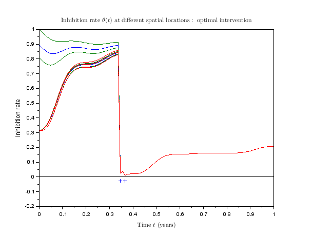
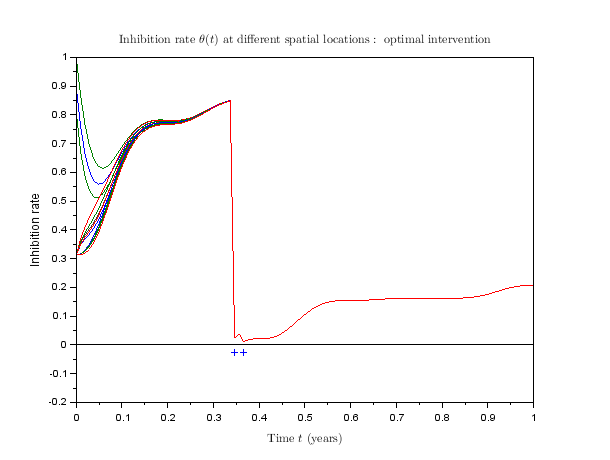
Refer to caption
Fig. 5: Inhibition rate with optimal pulse control as a function of time for different grid points on a 10×10×310\times 10\times 3 grid, for a system with A=I,c=0.55,Cf=0,A=I,c=0.55,C_{f}=0, and other parameters as given in Tables I and II. The space-averaged version of this system is associated with the c=0.55c=0.55 curve in Figure 2. Note the optimal pulse interventions (indicated by the markings below the time axis) are the same in both cases.
Refer to caption
Fig. 6: Inhibition rate with optimal pulse control for different grid points, for a system as in Figure 5 except with diffusion matrix A=10​IA=10I.

Next, we consider the case where the inhibition pressure depends on spatial location. We did this by choosing a⁡(x)a(x) in (56) for each grid point independently according to a uniform random distribution, then rescaling so that the average value of a⁡(x)a(x) agrees with Table I. Other parameters from Table I remain unchanged, and are constant with respect to the space variable. In particular, the initial conditions ρ⁡(x)\rho(x) were taken as constant with respect to the space variable. Figure 7 shows the inhibition rate as a function of time for all grid points of a 10×10×310\times 10\times 3 grid when optimal pulse control is applied. Unlike the cases shown in Figures 5 and  6, in this case the optimal strategy depends on spatial position.

Refer to caption
Fig. 7: Inhibition rate with optimal pulse control for a system as in Figure 5 except with constant initial inhibition pressure, and with space-dependent inhibition rate.

VII Discussion

This paper significantly extends the results of [14] in several respects. First, the model has been generalized by imposing weaker smoothness conditions on the parameters. Parameters are only required to be measurable and essentially locally bounded on ℝ3+1\mathbb{R}^{3+1}. Under these conditions, we have showed existence and uniqueness of a solution which takes values in [0,1]\left[0,1\right], thus establishing the model to be well formulated mathematically and epidemiologically. Second, we have included the possibility of a pulse control strategy, along with the continuous (chemical) control strategy studied in [14]. The added pulse strategy v=(vi)i∈ℕv=\left(v_{i}\right)_{i\in\mathbb{N}} represents the cultivational practices such as pruning old infected twigs, removing mummified fruits [5, 19, 20, 21, 28]. Third, we have verified an explicit algorithm for finding the optimal pulse-only strategy in the case where σ∗=0\sigma^{\ast}=0. Numerical simulations for both the averaged version of the model and the full version confirm the practical applicability of this algorithm. As explained in subsection III-A, the averaged version of the model faithfully represents the average behavior on the bounded domain Ω\Omega, when inhibition pressure and intervention costs are space-independent.

Practical computation of control strategies that optimize the use of both pulse and chemical contr are the subject of ongoing research.

ACKNOWLEDGEMENTS

The author thank Doctor Martial NDEFFO MBAH from the Yale School of Medecine and the University of Cambridge for all his useful remarks concerning the presentation of the paper. They also thank the African Mathematics Millennium Science Initiative (AMMSI) for the financial support they gave to the first author in the year 2014.

References

  • [1] ANITA S., ARNAUTU V., CAPASSO V., An Introduction to Optimal Control Problems in Life Scienes and Economics, Springer Science+Business Media, New York, 2011.
  • [2] BARBU V., Partial Differential Equations and Boundary Value Problems, Kluwer Academic Publishers, Dordrecht, 1998.
  • [3] BELLA-MANGA, BIEYSS D., MOUEN B., NYASS S., BERRY D., Elaboration d’une stratégie de lutte durable et efficace contre l’anthracnose des baies du caféier arabica dans les hautes terres de l’Ouest-Cameroun: bilan des connaissances acquises et perspectives, COLLOQUE Scientifique International sur le Café, 19, Trieste, Mai 2001.
  • [4] BIEYSSE D., BELLA-MANGA D., MOUEN B., NDEUMENI J., ROUSSEL J., FABRE V. and BERRY D., L’anthracnose des baies une menace potentielle pour la culture mondiale de l’arabica. plantations, recherche, développement, pp 145-152, 2002.
  • [5] BOISSON C., L’anthracnose du caféier, revue de mycologie, 1960.
  • [6] BREZIS H., Functional Analysis, Sobolev Spaces and Partial Differential Equations, Springer Science+Business Media, New York, 2011.
  • [7] CHEN Z., NUNES M., SILVA M., RODRIGUEZ J., Appressorium turgor pressure of Colletotrichum kahawae might have a role in coffee cuticle penetration, mycologia, 96(6), pp. 1199–1208, 2004.
  • [8] BENZONI-GAVAGE S., Calcul Différentiel et Équations Différentielles, Dunod, Paris, 2010.
  • [9] CODDINGTON E., LEVINSON N., Theory of Ordinary Differential Equations, McGraw-Hill, New York, 1955.
  • [10] DANNEBERGER T., VARGAS J., JONES Jr., and JONES A., A model for weather-based forecasting of anthracnose on annual bluegrass, Phytopathology, Vol. 74, No. 4, pp 448-451, 1984.
  • [11] DODD J., ESTRADA A., MATCHAM J., JEFFRIES P., JEGER J., The effect of climatic factors on Colletotrichum gloeosporioides, causal agent of mango anthracnose, in the Philippines, Plant Pathology (40), pp 568-575, 1991.
  • [12] DURAND N., BERTRAND B., GUYOT B., GUIRAUD J. & FONTANA T., Study on the coffea arabica/Colletotrichum kahawae pathosystem: Impact of a biological plant protection product, J.Plant Dis.Protect. , 116 (2), pp 78–85, 2009.
  • [13] DUTHIE J., Models of the response of foliar parasites to the combined effects of temperature and duration of wetness, Phytopathology, Vol. 87, No. 11, 1997.
  • [14] FOTSA D., HOUPA E., BEKOLLE D., THRON C., NDOUMBE M., Mathematical modelling and optimal control of anthracnose, Biomath, Vol. 3, 2014.
  • [15] GANESH D., PETITOT A., SILVA M., ALARY R., LECOULS A., FERNANDEZ D., Monitoring of the early molecular resistance responses of coffee (coffea arabica L.) to the rust fungus (hemileia vastatrix) using real-time quantitative RT-PCR, Plant Science 170, pp 1045–1051, 2006.
  • [16] JEFFRIES P., DODD J., JEGER M., PLUMBLEY R., The biology and the control of Colletotrichum spieces on tropical fruit crops, Plant Pathology (39), pp 343-366, 1990.
  • [17] MOUEN B., BIEYSSE D., CILAS C., and NOTTEGHEM J., Spatio-temporal dynamics of arabica coffee berry disease caused by Colletotrichum kahawae on a plot scale. Plant Dis. 91: 1229-1236, 2007.
  • [18] MOUEN B., BIEYSSE D., NYASSE S., NOTTEGHEM J., and CILAS C., Role of rainfall in the development of coffee berry disease in coffea arabica caused by Colletotrichum kahawae, in cameroon, Plant pathology, 2009.
  • [19] MOUEN B., BIEYSSE D., NJIAYOUOM I., DEUMENI J., CILAS C., and NOTTEGHEM J.,Effect of cultural practices on the development of arabica coffee berry disease, caused by Colletotrichum kahawae, Eur J Plant Pathol. 119: 391–400, 2007.
  • [20] MOUEN B., CHILLET M., JULLIEN A., BELLAIRE L., Le gainage précoce des régimes de bananes améliore la croissance des fruits et leur état sanitaire vis-à-vis de l’anthracnose (Colletotrichum musae), fruits, vol. 58, p. 71–81, 2003.
  • [21] MOUEN B., NJIAYOUOM I., BIEYSSE D., NDOUMBE N., CILAS C., and NOTTEGHEM J., Effect of shade on arabica coffee berry disease development: Toward an agroforestry system to reduce disease impact, Phytopathology, Vol. 98, No. 12, 2008.
  • [22] MULLER R., GESTIN A., Contribution à la mise au point des méthodes de lutte contrel’anthracnose des baies du caféier d’arabie (coffea arabica) due à une forme du Colletotrichum coffeanum Noack au Cameroun, café cacao thé, vol. XI (2), 1967.
  • [23] MULLER R., L’évolution de l’anthracnose des baies du caféier d’arabie (coffea arabica) due à une forme du Colletotrichum coffeanum Noack au Cameroun, café cacao thé, vol. XIV (2), 1970.
  • [24] MULLER R., La lutte contre l’anthracnose des baies du caféier arabica due à une souche de Colletotrichum coffeanum au Cameroun, note technique, institut français du café, du cacao et autres plantes stimulantes, 1971.
  • [25] PRESS W., TEUKOLSKY S., VETTERLING W., FLANNERY B., Numerical Recipes in C : The Art of Scientific Computing, Second Edition, Cambridge University Press, New York, 1992.
  • [26] RAMOS A. and KAMIDI R., Determination and significance of the mutation rate of Colletotrichum coffeanum from benomyl sensitivity to benomyl tolerance, phytopathology, vol. 72, N∘. 2, 1982.
  • [27] SILVA M., VÁRZEA V., GUERRA-GUIMARÃES L., AZINEIRA G., FERNANDEZ D., PETITOT A., BERTRAND B., LASHERMES P. and NICOLE M., Coffee resistance to the main diseases: leaf rust and coffee berry disease, Braz. J. Plant Physiol., 18(1): 119-147, 2006.
  • [28] WHARTON P., DIEGUEZ-URIBEONDO J., The biology of Colletotrichum acutatum, Anales del Jardín Botánico de Madrid 61(1): 3-22, 2004.