跳到论文正文
W Papers独立论文阅读器 arXiv:1406.3810 论文正文 计算阅读时间 · 0%
引用这篇论文根据当前论文元数据生成,正式投稿前建议核对。


License: arXiv.org perpetual non-exclusive license
arXiv:1406.3810v1 [math.AP] 15 Jun 2014

On the classical limit of a time-dependent self-consistent field system: analysis and computationThanks: This work was partially supported by NSF grants DMS-1114546 and DMS-1107291: NSF Research Network in Mathematical Sciences KI-Net: Kinetic description of emerging challenges in multiscale problems of natural sciences. C.S. acknowledges support by the NSF through grant numbers DMS-1161580 and DMS-1348092

Shi Jin S. JinDepartment of Mathematics, Institute of Natural Sciences and MOE Key Lab in Scientific and Engineering Computing, Shanghai Jiao Tong University, 800 Dong Chuan Road, Shanghai 200240, China & Department of Mathematics, University of Wisconsin-Madison, 480 Lincoln Drive, Madison, WI 53706, USA. Email address: jin@math.wisc.edu , Christof Sparber Z. ZhouDepartment of Mathematics, University of Wisconsin-Madison, 480 Lincoln Drive, Madison, WI 53706, USA. Email address: zhou@math.wisc.edu and Zhennan Zhou C. SparberDepartment of Mathematics, Statistics, and Computer Science, M/C 249, University of Illinois at Chicago, 851 S. Morgan Street, Chicago, IL 60607, USA. Email address: sparber@math.uic.edu
Date: August 24, 2026
Abstract.

We consider a coupled system of Schrödinger equations, arising in quantum mechanics via the so-called time-dependent self-consistent field method. Using Wigner transformation techniques we study the corresponding classical limit dynamics in two cases. In the first case, the classical limit is only taken in one of the two equations, leading to a mixed quantum-classical model which is closely connected to the well-known Ehrenfest method in molecular dynamics. In the second case, the classical limit of the full system is rigorously established, resulting in a system of coupled Vlasov-type equations. In the second part of our work, we provide a numerical study of the coupled semi-classically scaled Schrödinger equations and of the mixed quantum-classical model obtained via Ehrenfest’s method. A second order (in time) method is introduced for each case. We show that the proposed methods allow time steps independent of the semi-classical parameter(s) while still capturing the correct behavior of physical observables. It also becomes clear that the order of accuracy of our methods can be improved in a straightforward way.

Key words and phrases: 
Quantum mechanics, classical limit, self-consistent field method, Wigner transform, Ehrenfest method, time-splitting algorithm
2000 Mathematics Subject Classification
35Q41, 35B40, 65M70, 35Q83

1. Introduction

The numerical simulation of many chemical, physical, and biochemical phenomena requires the direct simulation of dynamical processes within large systems involving quantum mechanical effects. However, if the entire system is treated quantum mechanically, the numerical simulations are often restricted to relatively small model problems on short time scales due to the formidable computational cost. In order to overcome this difficulty, a basic idea is to separate the involved degrees of freedom into two different categories: one, which involves variables that behave effectively classical (i.e., evolving on slow time- and large spatial scales) and one which encapsulates the (fast) quantum mechanical dynamics within a certain portion of the full system. For example, for a system consisting of many molecules, one might designate the electrons as the fast degrees of freedom and the atomic nuclei as the slow degrees of freedom.

Whereas separation of the whole system into a classical part and a quantum mechanical part is certainly not an easy task, it is, by now, widely studied in the physics literature and often leads to what is called time-dependent self-consistent field equations (TDSCF), see, e.g., [5, 7, 13, 19, 24] and the references therein. In the TDSCF method, one typically assumes that the total wave function of the system Ψ⁡(t,X)\Psi(t,X), with X=(x,y)X=(x,y), can be approximated by

Ψ⁡(X,t)≈ψ⁡(x,t)​φ​(y,t),\Psi(X,t)\approx\psi(x,t)\varphi(y,t),

where xx and yy denote the degrees of freedom within a certain subsystem, only. The precise nature of this approximation thereby strongly depends on the concrete problem at hand. Disregarding this issue for the moment, one might then, in a second step, hope to derive a self-consistently coupled system for ψ\psi and φ\varphi and approximate it, at least partially, by the associated classical dynamics.

In this article we will study a simple model problem for such a TDSCF system, motivated by [7], but one expects that our findings extend to other self-consistent models as well. We will be interested in deriving various (semi-)classical approximations to the considered TDSCF system, resulting in either a mixed quantum-classical model, or a fully classical model. As we shall see, this also gives a rigorous justification of what is known as the Ehrenfest method in the physics literature, cf. [5, 7]. To this end, we shall be heavily relying on Wigner transformation techniques, developed in [9, 20], which have been proved to be superior in many aspects to the more classical WKB approximations, see, e.g. [23] for a broader discussion. One should note that the use of Wigner methods to study the classical limit of nonlinear (self-consistent) quantum mechanical models is not straightforward and usually requires additional assumptions on the quantum state, cf. [21, 20]. It turns out that in our case we can get by without them.

In the second part of this article we shall then be interested in designing an efficient and accurate numerical method which allows us to pass to the classical limit in the TDSCF system within our numerical algorithm. We will be particularly interested in the meshing strategy required to accurately approximate the wave functions, or to capture the correct physical observables (which are quadratic quantities of the wave function). To this end, we propose a second order (in time) method based on an operator splitting and a spectral approximation of the TDSCF equations as well as the obtained Ehrenfest model. These types of methods have been proven to be very effective in earlier numerical studies, see [2, 18, 3, 16] for previous results and [15] for a review of the current state-of-the art of numerical methods for semi-classical Schrödinger type models. In comparison to the case of a single (semi-classical) nonlinear Schrödinger equation with power law nonlinearities, where on has to use time steps which are comparable to the size of the small semi-classical parameter (see [2]), it turns out that in our case, despite of the nonlinearity, we can rigorously justify that one can take time steps independent of the semi-classical parameter and still capture the correct classical limit of physical observables.

The rest of this paper is now organized as follows: In Section 2, we present the considered TDSCF system and discuss some of its basic mathematical properties, which will be used later on. In Section 3, a brief introduction to the Wigner transforms and Wigner measures is given. In Section 4 we study the semi-classical limit, resulting in a mixed quantum-classical limit system. In Section 5 the completely classical approximation of the TDSFC system is studied by means of two different limiting processes, both of which result in the same classical model. The numerical methods used for the TDSCF equations and the Ehrenfest equations are then introduced in Section 6. Finally, we study several numerical tests cases in Section 7 in order to verify the properties of our methods.

2. The TDSCF system

2.1. Basic set-up and properties

In the following, we take x∈ℝdx\in{\mathbb{R}}^{d}, y∈ℝny\in{\mathbb{R}}^{n}, with d,n∈ℕd,n\in{\mathbb{N}}, and denote by ⟨⋅,⋅⟩Lx2\langle\cdot,\cdot\rangle_{L_{x}^{2}} and ⟨⋅,⋅⟩Ly2\langle\cdot,\cdot\rangle_{L_{y}^{2}} the usual inner product in L2​(ℝxd)L^{2}({\mathbb{R}}^{d}_{x}) and L2​(ℝyn)L^{2}({\mathbb{R}}^{n}_{y}), respectively, i.e.

⟨f,g⟩Lz2≡∫ℝmf¯​(z)​g​(z)​𝑑z.\left\langle f,g\right\rangle_{L_{z}^{2}}\equiv\int_{{\mathbb{R}}^{m}}\bar{f}(z)g(z)dz.

The total Hamiltonian of the system acting on L2​(ℝd+n)L^{2}({\mathbb{R}}^{d+n}) is assumed to be of the form

(2.1) H=−δ22​Δx−ε22​Δy+V⁡(x,y),H=-\frac{\delta^{2}}{2}\Delta_{x}-\frac{\varepsilon^{2}}{2}\Delta_{y}+V(x,y),

where V⁡(x,y)∈ℝV(x,y)\in{\mathbb{R}} is some (time-independent) real-valued potential. Typically, one has

(2.2) V⁡(x,y)=V1​(x)+V2​(y)+W⁡(x,y),V(x,y)=V_{1}(x)+V_{2}(y)+W(x,y),

where V1,2V_{1,2} are external potentials acting only on the respective subsystem and WW represents an internal coupling potential in between the two subsystems. From now on, we shall assume that VV is smooth and rapidly decaying at infinity, i.e.

(2.3) V∈𝒮⁡(ℝxd×ℝyn).V\in\mathcal{S}({\mathbb{R}}^{d}_{x}\times{\mathbb{R}}^{n}_{y}).

In particular, we may, without restriction of generality, assume V⁡(x,y)⩾0V(x,y)\geqslant 0.

Remark 2.1.

The proofs given below will show that, with some effort, all of our results can be extended to the case of potentials V∈Cb2​(ℝxd×ℝyn)V\in C^{2}_{\rm b}({\mathbb{R}}^{d}_{x}\times{\mathbb{R}}^{n}_{y}).

In (2.1), the Hamiltonian is already written in dimensionless form, such that only two (small) parameters ε,δ>0\varepsilon,\delta>0 remain. In the following, they play the role of dimensionless Planck’s constants. Dependence with respect to these parameters will be denoted by superscripts. The TDSCF system at hand is then (formally given by [7]) the following system of self-consistently coupled Schrödinger equations

(2.4) {iδ∂tψε,δ=(−δ22Δx+⟨φε,δ,Vφε,δ⟩Ly2)ψε,δ,ψε,δ∣t=0=ψδin(x),iε∂tφε,δ=(−ε22Δy+⟨ψε,δ,hδψε,δ⟩Lx2)φε,δ,φε,δ∣t=0=φεin(y),\left\{\begin{split}i\delta\partial_{t}\psi^{\varepsilon,\delta}=\left(-\frac{\delta^{2}}{2}\Delta_{x}+\langle\varphi^{\varepsilon,\delta},V\varphi^{\varepsilon,\delta}\rangle_{L_{y}^{2}}\right)\psi^{\varepsilon,\delta}\,,\quad\psi^{\varepsilon,\delta}_{\mid t=0}=\psi^{\delta}_{\rm in}(x),\\ i\varepsilon\partial_{t}\varphi^{\varepsilon,\delta}=\left(-\frac{\varepsilon^{2}}{2}\Delta_{y}+\langle\psi^{\varepsilon,\delta},h^{\delta}\psi^{\varepsilon,\delta}\rangle_{L_{x}^{2}}\right)\varphi^{\varepsilon,\delta}\,,\quad\varphi^{\varepsilon,\delta}_{\mid t=0}=\varphi^{\varepsilon}_{\rm in}(y),\end{split}\right.

where we denote by

(2.5) hδ=−δ22​Δx+V⁡(x,y),h^{\delta}=-\frac{\delta^{2}}{2}\Delta_{x}+V(x,y),

the Hamiltonian of the subsystem represented by the xx-variables (considered as the purely quantum mechanical variables) and in which yy only enters as a parameter. For simplicity, we assume that at t=0t=0 the data ψinδ\psi_{\rm in}^{\delta} only depends on δ\delta, and that φinε\varphi_{\rm in}^{\varepsilon} only depends on ε\varepsilon, which means that the simultaneous dependence on both parameters is only induced by the time-evolution. Finally, the coupling terms are explicitly given by

⟨φε,δ,V​φε,δ⟩Ly2=∫ℝynV⁡(x,y)​|φε,δ​(y,t)|2​𝑑y=:Υε,δ​(x,t),\langle\varphi^{\varepsilon,\delta},V\varphi^{\varepsilon,\delta}\rangle_{L_{y}^{2}}=\int_{{\mathbb{R}}_{y}^{n}}V(x,y)|\varphi^{\varepsilon,\delta}(y,t)|^{2}\,dy=:\Upsilon^{\varepsilon,\delta}(x,t),

and after formally integrating by parts

⟨ψε,δ,hδ​ψε,δ⟩Lx2=∫ℝxdδ22​|∇ψε,δ​(x,t)|2+V⁡(x,y)​|ψε,δ​(x,t)|2​𝑑x=:Λε,δ​(y,t).\langle\psi^{\varepsilon,\delta},h^{\delta}\psi^{\varepsilon,\delta}\rangle_{L_{x}^{2}}=\int_{{\mathbb{R}}_{x}^{d}}\frac{\delta^{2}}{2}|\nabla\psi^{\varepsilon,\delta}(x,t)|^{2}+V(x,y)|\psi^{\varepsilon,\delta}(x,t)|^{2}\,dx=:\Lambda^{\varepsilon,\delta}(y,t).

Throughout this work we will always interpret the term ⟨ψε,δ,hδ​ψε,δ⟩Lx2\langle\psi^{\varepsilon,\delta},h^{\delta}\psi^{\varepsilon,\delta}\rangle_{L_{x}^{2}} as above, i.e., in the weak sense. Both Υε,δ\Upsilon^{\varepsilon,\delta} and Λε,δ\Lambda^{\varepsilon,\delta} are time-dependent, real-valued potentials, computed self-consistently via the dynamics of φε,δ\varphi^{\varepsilon,\delta} and ψε,δ\psi^{\varepsilon,\delta}, respectively. Note that

(2.6) Λε,δ​(y,t)=δ22​‖∇ψε,δ‖Lx22+⟨ψε,δ,V​ψε,δ⟩Lx2≡ϑε,δ​(t)+⟨ψε,δ,V​ψε,δ⟩Lx2.\Lambda^{\varepsilon,\delta}(y,t)=\frac{\delta^{2}}{2}\|\nabla\psi^{\varepsilon,\delta}\|^{2}_{L^{2}_{x}}+\langle\psi^{\varepsilon,\delta},V\psi^{\varepsilon,\delta}\rangle_{L_{x}^{2}}\equiv\vartheta^{\varepsilon,\delta}(t)+\langle\psi^{\varepsilon,\delta},V\psi^{\varepsilon,\delta}\rangle_{L_{x}^{2}}.

Here, the purely time-dependent part ϑε,δ​(t)\vartheta^{\varepsilon,\delta}(t), could in principle be absorbed into the definition of φε,δ\varphi^{\varepsilon,\delta} via a Gauge transformation, i.e.,

(2.7) φε,δ(x,t)↦φ~ε,δ(x,t):=φε,δ(x,t)exp(−iε∫0tϑε,δ(s)ds),\varphi^{\varepsilon,\delta}(x,t)\mapsto\widetilde{\varphi}^{\varepsilon,\delta}(x,t):={\varphi^{\varepsilon,\delta}}(x,t)\exp\left(-\frac{i}{\varepsilon}\int_{0}^{t}\vartheta^{\varepsilon,\delta}(s)\,ds\right),

For the sake of simplicity, we shall refrain from doing so, but this nevertheless shows that the two coupling terms are in essence of the same form. Also note that this Gauge transform leaves any Hs​(ℝd)H^{s}({\mathbb{R}}^{d})-norm of φε,δ\varphi^{\varepsilon,\delta} invariant (but clearly depends on the solution of the second equation within the TDSCF system).

Remark 2.2.

For potentials of the form (2.2), one can check that in the case where W⁡(x,y)≡0W(x,y)\equiv 0, i.e., no coupling term, one can use similar gauge transformations to completely decouple the two equations in (2.4) and obtain two linear Schrödinger equations in xx and yy, respectively.

An important physical quantity is the total masses of the system,

(2.8) Mε,δ​(t):=‖ψε,δ​(⋅,t)‖Lx22+‖φε,δ​(⋅,t)‖Ly22≡m1ε,δ​(t)+m2ε,δ​(t).M^{\varepsilon,\delta}(t):=\|\psi^{\varepsilon,\delta}(\cdot,t)\|^{2}_{L_{x}^{2}}+\|\varphi^{\varepsilon,\delta}(\cdot,t)\|^{2}_{L_{y}^{2}}\equiv m_{1}^{\varepsilon,\delta}(t)+m_{2}^{\varepsilon,\delta}(t).

where m1ε,δm_{1}^{\varepsilon,\delta}, m2ε,δm_{2}^{\varepsilon,\delta} denote the masses of the respective subsystem. One can then prove that these are conserved by the time-evolution of (2.4).

Lemma 2.3.

Assume that ψε,δ∈C⁡(ℝt,H1​(ℝxd))\psi^{\varepsilon,\delta}\in C({\mathbb{R}}_{t};H^{1}({\mathbb{R}}^{d}_{x})) and φε,δ∈C⁡(ℝt,L2​(ℝyn))\varphi^{\varepsilon,\delta}\in C({\mathbb{R}}_{t};L^{2}({\mathbb{R}}^{n}_{y})) solve (2.4), then

m1ε,δ​(t)=m1ε,δ​(0),m2ε,δ​(t)=m2ε,δ​(0),∀t∈ℝ.m_{1}^{\varepsilon,\delta}(t)=m_{1}^{\varepsilon,\delta}(0),\quad m_{2}^{\varepsilon,\delta}(t)=m_{2}^{\varepsilon,\delta}(0),\quad\forall\,t\in{\mathbb{R}}.
Proof.

Assuming for the moment, that both ψε,δ\psi^{\varepsilon,\delta} and φε,δ\varphi^{\varepsilon,\delta} are sufficiently smooth and decaying, we multiply the first equation in (2.4) with ψε,δ¯\overline{\psi^{\varepsilon,\delta}} and formally integrate with respect to x∈ℝxdx\in{\mathbb{R}}^{d}_{x}. Taking the real part of the resulting expression and having in mind that Υε,δ​(y,t)∈ℝ\Upsilon^{\varepsilon,\delta}(y,t)\in{\mathbb{R}}, yields

dd​t​m1ε,δ​(t)≡dd​t​‖ψε,δ​(⋅,t)‖Lx22=0,\frac{d}{dt}m_{1}^{\varepsilon,\delta}(t)\equiv\frac{d}{dt}\|\psi^{\varepsilon,\delta}(\cdot,t)\|_{L^{2}_{x}}^{2}=0,

which, after another integration in time, is the desired result for m1ε,δ​(t)m_{1}^{\varepsilon,\delta}(t). By the same argument one can show the result for m2ε,δ​(t)m_{2}^{\varepsilon,\delta}(t). Integration in time in combination with a density argument then allows to extend the result to more general solutions in H1H^{1} and L2L^{2}, respectively. ∎

We shall, from now on assume that the initial data is normalized such that m1ε,δ​(0)=m2ε,δ​(0)=1m_{1}^{\varepsilon,\delta}(0)=m_{2}^{\varepsilon,\delta}(0)=1. Using this normalization, the total energy of the system can be written as

(2.9) Eε,δ​(t):=δ22​‖∇ψε,δ​(⋅,t)‖Lx22+ε22​‖∇φε,δ​(⋅,t)‖Ly22+∬ℝd+nV(x,y)|ψε,δ(x,t)|2|φε,δ(y,t)|2dxdy.\begin{split}E^{\varepsilon,\delta}(t):=&\,\frac{\delta^{2}}{2}\|\nabla\psi^{\varepsilon,\delta}(\cdot,t)\|^{2}_{L^{2}_{x}}+\frac{\varepsilon^{2}}{2}\|\nabla\varphi^{\varepsilon,\delta}(\cdot,t)\|^{2}_{L^{2}_{y}}\\ &\,+\iint_{{\mathbb{R}}^{d+n}}V(x,y)|\psi^{\varepsilon,\delta}(x,t)|^{2}|\varphi^{\varepsilon,\delta}(y,t)|^{2}\,dx\,dy.\end{split}
Lemma 2.4.

Assume that ψε,δ∈C⁡(ℝt,H1​(ℝxd))\psi^{\varepsilon,\delta}\in C({\mathbb{R}}_{t};H^{1}({\mathbb{R}}^{d}_{x})) and φε,δ∈C⁡(ℝt,H1​(ℝyn))\varphi^{\varepsilon,\delta}\in C({\mathbb{R}}_{t};H^{1}({\mathbb{R}}^{n}_{y})) solve (2.4), then

Eε,δ​(t)=Eε,δ​(0),∀t∈ℝ.E^{\varepsilon,\delta}(t)=E^{\varepsilon,\delta}(0),\quad\forall\,t\in{\mathbb{R}}.
Proof.

Assuming, as before that ψε,δ\psi^{\varepsilon,\delta} and φε,δ\varphi^{\varepsilon,\delta} are sufficiently regular (and decaying), the proof is a lengthy but straightforward calculation. More precisely, using the shorthand

Eε,δ​(t)=δ22​‖∇ψε,δ​(⋅,t)‖Lx22+ε22​‖∇φε,δ​(⋅,t)‖Ly22+⟨ψε,δ​φε,δ,V​ψε,δ​φε,δ⟩Lx,y2,E^{\varepsilon,\delta}(t)=\frac{\delta^{2}}{2}\|\nabla\psi^{\varepsilon,\delta}(\cdot,t)\|^{2}_{L^{2}_{x}}+\frac{\varepsilon^{2}}{2}\|\nabla\varphi^{\varepsilon,\delta}(\cdot,t)\|^{2}_{L^{2}_{y}}+\langle\psi^{\varepsilon,\delta}\varphi^{\varepsilon,\delta},V\psi^{\varepsilon,\delta}\varphi^{\varepsilon,\delta}\rangle_{L^{2}_{x,y}},

one finds that

dd​t​Eε,δ​(t)=(I)+(II)+(III)+(IV),\frac{d}{dt}E^{\varepsilon,\delta}(t)=(\rm{I})+(\rm{II})+(\rm{III})+(\rm{IV}),

where we denote

(I):=\displaystyle({\rm I}):= δ22⟨∇x∂tψε,δ,∇xψε,δ⟩Lx2+δ22⟨∇xψε,δ,∇x∂tψε,δ⟩Lx2,\displaystyle\frac{\delta^{2}}{2}\langle\nabla_{x}\partial_{t}\psi^{\varepsilon,\delta},\nabla_{x}\psi^{\varepsilon,\delta}\rangle_{L^{2}_{x}}+\frac{\delta^{2}}{2}\langle\nabla_{x}\psi^{\varepsilon,\delta},\nabla_{x}\partial_{t}\psi^{\varepsilon,\delta}\rangle_{L^{2}_{x}},
(II):=\displaystyle({\rm II}):= ε22⟨∇y∂tφε,δ,∇yφε,δ⟩Ly2+ε22⟨∇yφε,δ,∇y∂tφε,δ⟩Ly2,\displaystyle\frac{\varepsilon^{2}}{2}\langle\nabla_{y}\partial_{t}\varphi^{\varepsilon,\delta},\nabla_{y}\varphi^{\varepsilon,\delta}\rangle_{L^{2}_{y}}+\frac{\varepsilon^{2}}{2}\langle\nabla_{y}\varphi^{\varepsilon,\delta},\nabla_{y}\partial_{t}\varphi^{\varepsilon,\delta}\rangle_{L^{2}_{y}},
(III):=\displaystyle({\rm III}):= ⟨∂tψε,δ​φε,δ,V​ψε,δ​φε,δ⟩Lx,y2+⟨ψε,δ​φε,δ,V​∂tψε,δ​φε,δ⟩Lx,y2,\displaystyle\langle\partial_{t}\psi^{\varepsilon,\delta}\varphi^{\varepsilon,\delta},V\psi^{\varepsilon,\delta}\varphi^{\varepsilon,\delta}\rangle_{L^{2}_{x,y}}+\langle\psi^{\varepsilon,\delta}\varphi^{\varepsilon,\delta},V\partial_{t}\psi^{\varepsilon,\delta}\varphi^{\varepsilon,\delta}\rangle_{L^{2}_{x,y}},
(IV):=\displaystyle({\rm IV}):= ⟨ψε,δ​∂tφε,δ,V​ψε,δ​φε,δ⟩Lx,y2+⟨ψε,δ​φε,δ,V​ψε,δ​∂tφε,δ⟩Lx,y2.\displaystyle\langle\psi^{\varepsilon,\delta}\partial_{t}\varphi^{\varepsilon,\delta},V\psi^{\varepsilon,\delta}\varphi^{\varepsilon,\delta}\rangle_{L^{2}_{x,y}}+\langle\psi^{\varepsilon,\delta}\varphi^{\varepsilon,\delta},V\psi^{\varepsilon,\delta}\partial_{t}\varphi^{\varepsilon,\delta}\rangle_{L^{2}_{x,y}}.

We will now show that (I)+(III)=0(\rm{I})+(\rm{III})=0. By using the (2.4), one gets

(I)\displaystyle({\rm I}) =\displaystyle= −δ2​i​⟨∇x(−δ22​Δx+⟨φε,δ,V​φε,δ⟩Ly2)​ψε,δ,∇xψε,δ⟩Lx2\displaystyle-\frac{\delta}{2i}\left\langle\nabla_{x}\left(-\frac{\delta^{2}}{2}\Delta_{x}+\langle\varphi^{\varepsilon,\delta},V\varphi^{\varepsilon,\delta}\rangle_{L^{2}_{y}}\right)\psi^{\varepsilon,\delta},\nabla_{x}\psi^{\varepsilon,\delta}\right\rangle_{L^{2}_{x}}
+δ2​i​⟨∇xψε,δ,∇x(−δ22​Δx+⟨φε,δ,V​φε,δ⟩Ly2)​ψε,δ⟩Lx2\displaystyle+\frac{\delta}{2i}\left\langle\nabla_{x}\psi^{\varepsilon,\delta},\nabla_{x}\left(-\frac{\delta^{2}}{2}\Delta_{x}+\langle\varphi^{\varepsilon,\delta},V\varphi^{\varepsilon,\delta}\rangle_{L^{2}_{y}}\right)\psi^{\varepsilon,\delta}\right\rangle_{L^{2}_{x}}
=\displaystyle= −δ2​i​⟨(∇x⟨φε,δ,V​φε,δ⟩Ly2)​ψε,δ,∇xψε,δ⟩Lx2\displaystyle-\frac{\delta}{2i}\langle(\nabla_{x}\langle\varphi^{\varepsilon,\delta},V\varphi^{\varepsilon,\delta}\rangle_{L^{2}_{y}})\ \psi^{\varepsilon,\delta},\nabla_{x}\psi^{\varepsilon,\delta}\rangle_{L^{2}_{x}}
+δ2​i​⟨∇xψε,δ,(∇x⟨φε,δ,V​φε,δ⟩Ly2)​ψε,δ⟩Lx2\displaystyle+\frac{\delta}{2i}\langle\nabla_{x}\psi^{\varepsilon,\delta},(\nabla_{x}\langle\varphi^{\varepsilon,\delta},V\varphi^{\varepsilon,\delta}\rangle_{L^{2}_{y}})\ \psi^{\varepsilon,\delta}\rangle_{L^{2}_{x}}
=\displaystyle= δ2​i​⟨ψε,δ,[⟨φε,δ,V​φε,δ⟩Ly2,Δx]​ψε,δ⟩Lx2,\displaystyle\frac{\delta}{2i}\left\langle\psi^{\varepsilon,\delta},\left[\langle\varphi^{\varepsilon,\delta},V\varphi^{\varepsilon,\delta}\rangle_{L^{2}_{y}},\Delta_{x}\right]\psi^{\varepsilon,\delta}\right\rangle_{L^{2}_{x}},

where [A,B]:=A​B−B​A[A,B]:=AB-BA denotes the commutator bracket. Similarly, one finds that

(III)\displaystyle({\rm III}) =\displaystyle= −δ2​i​⟨(−δ22​Δx+⟨φε,δ,V​φε,δ⟩Ly2)​ψε,δ​ϕε,δ,V​ψε,δ​ϕε,δ⟩Lx,y2\displaystyle-\frac{\delta}{2i}\left\langle\left(-\frac{\delta^{2}}{2}\Delta_{x}+\langle\varphi^{\varepsilon,\delta},V\varphi^{\varepsilon,\delta}\rangle_{L^{2}_{y}}\right)\psi^{\varepsilon,\delta}\phi^{\varepsilon,\delta},V\psi^{\varepsilon,\delta}\phi^{\varepsilon,\delta}\right\rangle_{L^{2}_{x,y}}
+δ2​i​⟨ψε,δ​ϕε,δ,V⁡(−δ22​Δx+⟨φε,δ,V​φε,δ⟩y)​ψε,δ​ϕε,δ⟩Lx,y2\displaystyle+\frac{\delta}{2i}\left\langle\psi^{\varepsilon,\delta}\phi^{\varepsilon,\delta},V\left(-\frac{\delta^{2}}{2}\Delta_{x}+\langle\varphi^{\varepsilon,\delta},V\varphi^{\varepsilon,\delta}\rangle_{y}\right)\psi^{\varepsilon,\delta}\phi^{\varepsilon,\delta}\right\rangle_{L^{2}_{x,y}}
=\displaystyle= δ2​i​⟨Δx​ψε,δ,⟨φε,δ,V​φε,δ⟩y​ψε,δ⟩Lx2\displaystyle\frac{\delta}{2i}\left\langle\Delta_{x}\psi^{\varepsilon,\delta},\langle\varphi^{\varepsilon,\delta},V\varphi^{\varepsilon,\delta}\rangle_{y}\psi^{\varepsilon,\delta}\right\rangle_{L^{2}_{x}}
−δ2​i​⟨ψε,δ,⟨φε,δ,V​φε,δ⟩y​Δx​ψε,δ⟩Lx2\displaystyle-\frac{\delta}{2i}\left\langle\psi^{\varepsilon,\delta},\langle\varphi^{\varepsilon,\delta},V\varphi^{\varepsilon,\delta}\rangle_{y}\Delta_{x}\psi^{\varepsilon,\delta}\right\rangle_{L^{2}_{x}}
=\displaystyle= δ2​i​⟨ψε,δ,[Δx,⟨φε,δ,V​φε,δ⟩y]​ψε,δ⟩Lx2=−(I),\displaystyle\frac{\delta}{2i}\left\langle\psi^{\varepsilon,\delta},\left[\Delta_{x},\langle\varphi^{\varepsilon,\delta},V\varphi^{\varepsilon,\delta}\rangle_{y}\right]\psi^{\varepsilon,\delta}\right\rangle_{L^{2}_{x}}=-({\rm I)},

due to the fact that [A,B]=−[B,A][A,B]=-[B,A]. Therefore, one concludes (I)+(III)=0(\rm{I})+(\rm{III})=0. Analogously, one can show that (II)+(IV)=0(\rm{II})+(\rm{IV})=0 and hence, an integration in time yields Eε,δ​(t)=Eε,δ​(0)E^{\varepsilon,\delta}(t)=E^{\varepsilon,\delta}(0). Using a density arguments allows to extend this result to more general solution in H1H^{1}. ∎

Note however, that the energies defined for the respective subsystems are in general not conserved, unless V⁡(x,y)=V1​(x)+V2​(y)V(x,y)=V_{1}(x)+V_{2}(y).

2.2. Existence of solutions

In this subsection, we shall establish global in-time existence of solutions to the TDSCF system (2.4). Since the dependence on ε\varepsilon and δ\delta does not play a role here, we shall suppress their appearance for the sake of notation.

Proposition 2.5.

Let V∈𝒮⁡(ℝxd×ℝyn)V\in\mathcal{S}({\mathbb{R}}^{d}_{x}\times{\mathbb{R}}^{n}_{y}) and ψin∈H1​(ℝxd)\psi_{\rm in}\in H^{1}({\mathbb{R}}^{d}_{x}), φin∈H1​(ℝyn)\varphi_{\rm in}\in H^{1}({\mathbb{R}}^{n}_{y}). Then there exists a global strong solution (ψ,φ)∈C⁡(ℝt,H1​(ℝd+n))(\psi,\varphi)\in C({\mathbb{R}}_{t};H^{1}({\mathbb{R}}^{d+n})) of (2.4), satisfying the conservation laws for mass and energy, as stated above.

Clearly, this also yields global existence for the system (2.4) with 0<ε,δ<10<\varepsilon,\delta<1 included.

Proof.

We shall first prove local (in-time) well-posedness of the initial value problem (2.4): To this end, we consider Ψ⁡(⋅,t)=(ψ⁡(⋅,t),φ⁡(⋅,t)):ℝd+n→ℂ2\Psi(\cdot,t)=(\psi(\cdot,t),\varphi(\cdot,t)):{\mathbb{R}}^{d+n}\to{\mathbb{C}}^{2} and define the associated L2​(ℝd+n)L^{2}({\mathbb{R}}^{d+n}) norm by

‖Ψ⁡(⋅,t)‖L22:=‖ψ⁡(⋅,t)‖Lx22+‖φ⁡(⋅,t)‖Ly22,\|\Psi(\cdot,t)\|^{2}_{L^{2}}:=\|\psi(\cdot,t)\|^{2}_{L^{2}_{x}}+\|\varphi(\cdot,t)\|^{2}_{L^{2}_{y}},

and consequently set H1​(ℝd+n):={Ψ∈L2​(ℝd+n):|∇Ψ|∈L2​(ℝd+n)}H^{1}({\mathbb{R}}^{d+n}):=\{\Psi\in L^{2}({\mathbb{R}}^{d+n})\,:\,|\nabla\Psi|\in L^{2}({\mathbb{R}}^{d+n})\}. Using this notation, the TDSCF system (2.4) can be written as

i​∂tΨ=ℍ​Ψ+f⁡(Ψ),i\partial_{t}\Psi=\mathbb{H}\Psi+f(\Psi),

where

ℍ:=(−12​Δx00−12​Δy),f⁡(Ψ):=(⟨φ,V​φ⟩Ly2​ψ00⟨ψ,h​ψ⟩Lx2​φ).\mathbb{H}:=\left(\begin{matrix}-\frac{1}{2}\Delta_{x}&0\\ 0&-\frac{1}{2}\Delta_{y}\end{matrix}\right),\quad f(\Psi):=\left(\begin{matrix}\langle\varphi,V\varphi\rangle_{L^{2}_{y}}\psi&0\\ 0&\langle\psi,h\psi\rangle_{L^{2}_{x}}\varphi\end{matrix}\right).

Clearly, ℍ\mathbb{H} is the generator of a strongly continuous unitary Schrödinger group U⁡(t):=e−i​t​ℍU(t):=e^{-it\mathbb{H}}, which can be used to rewrite the system using Duhamel’s formula as

(2.10) Ψ⁡(t,⋅)=U⁡(t)​Ψin​(⋅)−i​∫0tU⁡(t−s)​f​(Ψ⁡(⋅,s))​𝑑s.\Psi(t,\cdot)=U(t)\Psi_{\rm in}(\cdot)-i\int_{0}^{t}U(t-s)f(\Psi(\cdot,s))\,ds.

Following classical semi-group arguments, cf. [6], it suffices to show that f⁡(Ψ)f(\Psi) is locally Lipschitz in H1​(ℝd+n)H^{1}({\mathbb{R}}^{d+n}) in order to infer the existence of a unique local in-time solution Ψ∈C⁡([0,T),H1​(ℝd+n))\Psi\in C([0,T),H^{1}({\mathbb{R}}^{d+n})). This is not hard to show, since, for example:

‖f⁡(Ψ1)−f⁡(Ψ2)‖L2⩽‖V‖L∞​(‖Ψ1‖L22+‖Ψ2‖H12)​‖Ψ1−Ψ2‖L2,\displaystyle\|f(\Psi_{1})-f(\Psi_{2})\|_{L^{2}}\leqslant\|V\|_{L^{\infty}}(\|\Psi_{1}\|_{L^{2}}^{2}+\|\Psi_{2}\|_{H^{1}}^{2})\|\Psi_{1}-\Psi_{2}\|_{L^{2}},

in view of the fact that V∈𝒮V\in\mathcal{S}. A similar argument can be done for ‖∇f​(Ψ)‖L2\|\nabla f(\Psi)\|_{L^{2}} and hence, one gets that there exists a C=C⁡(V,‖Ψ1‖H1,‖Ψ2‖H1)>0C=C(V,\|\Psi_{1}\|_{H^{1}},\|\Psi_{2}\|_{H^{1}})>0 such that

‖f⁡(Ψ1)−f⁡(Ψ2)‖H1⩽C​‖Ψ1−Ψ2‖H1.\displaystyle\|f(\Psi_{1})-f(\Psi_{2})\|_{H^{1}}\leqslant C\|\Psi_{1}-\Psi_{2}\|_{H^{1}}.

Using this, [6, Theorem 3.3.9] implies the existence of a T=T⁡(‖Ψ‖H1)>0T=T(\|\Psi\|_{H^{1}})>0 and a unique solution Ψ∈C⁡([0,T),H1​(ℝd+n))\Psi\in C([0,T),H^{1}({\mathbb{R}}^{d+n})) of (2.10). It is then also clear, that this solution satisfies the conservation of mass and energy for all t∈[0,T)t\in[0,T). Moreover, the quoted theorem also implies that if T<+∞T<+\infty, then

(2.11) limt→T−‖Ψ⁡(⋅,t)‖H1=∞.\lim_{t\to T_{-}}\|\Psi(\cdot,t)\|_{H^{1}}=\infty.

However, having in mind the conservation laws for mass and energy stated in Lemmas 2.3 and 2.4 together with the fact that we assume w.l.o.g. V⁡(x,y)⩾0V(x,y)\geqslant 0, we immediately infer that ‖Ψ⁡(⋅,t)‖H1⩽C\|\Psi(\cdot,t)\|_{H^{1}}\leqslant C for all t∈ℝt\in{\mathbb{R}} and hence, the blow-up alternative (2.11) implies global in-time existence of the obtained solution. ∎

Remark 2.6.

Note that this existence result rests on the fact that the term Λε,δ​(y,t):=⟨ψε,δ,hδ​ψε,δ⟩Lx2\Lambda^{\varepsilon,\delta}(y,t):=\langle\psi^{\varepsilon,\delta},h^{\delta}\psi^{\varepsilon,\delta}\rangle_{L_{x}^{2}} is interpreted in a weak sense, see (2.6). In order to interpret it in a strong sense, one would need to require higher regularity, in particular ψε,δ∈H2​(ℝxd)\psi^{\varepsilon,\delta}\in H^{2}({\mathbb{R}}^{d}_{x}).

3. Review of Wigner transforms and Wigner measures

The use of Wigner transformation and Wigner measures in the analysis of (semi)-classical asymptotic is, by now, very well established. We shall in the following, briefly recall the main results developed in [20, 9] (see also [8, 21, 23] for further applications and discussions of Wigner measures):

Denote by {fε}0<ε⩽1\{f^{\varepsilon}\}_{0<\varepsilon\leqslant 1} a family of functions fε∈L2​(ℝd)f^{\varepsilon}\in L^{2}({\mathbb{R}}^{d}), depending continuously on a small parameter ε>0\varepsilon>0, and by

(ℱx→ξfε)(ξ)≡f^ε(ξ):=∫ℝdfε(x)e−ix⋅ξdx.(\mathcal{F}_{x\to\xi}f^{\varepsilon})(\xi)\equiv\widehat{f}^{\varepsilon}(\xi):=\int_{{\mathbb{R}}^{d}}f^{\varepsilon}(x)e^{-ix\cdot\xi}dx.

the corresponding Fourier transform. The associated ε\varepsilon-scaled Wigner transform is then given by [25]:

(3.1) wε​[fε]​(x,ξ):=1(2​π)d​∫ℝdfε​(x−ε2​z)​fε¯​(x+ε2​z)​ei​z⋅ξ​𝑑z.w^{\varepsilon}[f^{\varepsilon}](x,\xi):=\frac{1}{(2\pi)^{d}}\int_{{\mathbb{R}}^{d}}f^{\varepsilon}\left(x-\frac{\varepsilon}{2}z\right)\overline{f^{\varepsilon}}\left(x+\frac{\varepsilon}{2}z\right)e^{iz\cdot\xi}\,dz.

Clearly, one has

(ℱξ→zw)(x,z)=∫ℝdw(x,ξ)e−iz⋅ξdξ=fε(x+ε2z)fε¯(x−ε2z),(\mathcal{F}_{\xi\to z}w)(x,z)=\int_{{\mathbb{R}}^{d}}w(x,\xi)e^{-iz\cdot\xi}d\xi=f^{\varepsilon}\Big(x+\frac{\varepsilon}{2}z\Big)\overline{f^{\varepsilon}}\Big(x-\frac{\varepsilon}{2}z\Big),

and thus Plancherel’s theorem together with a simple change of variables yields

∥wε∥L2​(ℝ2​d)=ε−d(2π)−d/2∥fε∥L2​(ℝd)2.\|w^{\varepsilon}\|_{L^{2}({\mathbb{R}}^{2d})}=\varepsilon^{-d}(2\pi)^{-d/2}\|f^{\varepsilon}\|^{2}_{L^{2}({\mathbb{R}}^{d})}.

The real-valued function wε​(x,ξ)w^{\varepsilon}(x,\xi) acts as a quantum mechanical analogue for classical phase-space distributions. However, wε​(x,ξ)⩾̸0w^{\varepsilon}(x,\xi)\not\geqslant 0 in general. A straightforward computation shows that the position density associated to fεf^{\varepsilon} can be computed via

|fε​(x)|2=∫ℝdwε​(x,ξ)​𝑑ξ.|f^{\varepsilon}(x)|^{2}=\int_{{\mathbb{R}}^{d}}w^{\varepsilon}(x,\xi)\,d\xi.

Moreover, by taking higher order moments in ξ\xi one (formally) finds

εIm(f¯ε(x)∇fε(x))=∫ℝdξwε(x,ξ)dξ.\varepsilon\text{Im}(\overline{f}^{\varepsilon}(x)\nabla f^{\varepsilon}(x))=\int_{{\mathbb{R}}^{d}}\xi w^{\varepsilon}(x,\xi)\,d\xi.

and

ε2​|∇fε​(x)|2=∫ℝd|ξ|2​wε​(x,ξ)​𝑑ξ.\varepsilon^{2}|\nabla f^{\varepsilon}(x)|^{2}=\int_{{\mathbb{R}}^{d}}|\xi|^{2}w^{\varepsilon}(x,\xi)\,d\xi.

In order to make these computations rigorous, the integrals on the r.h.s. have to be understood in an appropriate sense, since wε∉L1​(ℝxm×ℝξm)w^{\varepsilon}\not\in L^{1}({\mathbb{R}}^{m}_{x}\times{\mathbb{R}}^{m}_{\xi}) in general, cf. [20] for more details.

It has been proved in [9, 20] that if fεf^{\varepsilon} is uniformly bounded in L2​(ℝd)L^{2}({\mathbb{R}}^{d}) as ε→0+\varepsilon\to 0_{+}, i.e., if

sup0<ε⩽1‖fε‖Lx2⩽C,\sup_{0<\varepsilon\leqslant 1}\|f^{\varepsilon}\|_{L_{x}^{2}}\leqslant C,

where C>0C>0 is an ε\varepsilon-independent constant, then the set of Wigner functions {wε}0<ε⩽1⊂𝒮′​(ℝxd×ℝξd)\{w^{\varepsilon}\}_{0<\varepsilon\leqslant 1}\subset\mathcal{S}^{\prime}({\mathbb{R}}^{d}_{x}\times{\mathbb{R}}^{d}_{\xi}) is weak∗ compact. Thus, up to extraction of sub-sequences, there exists a limiting object w0≡w∈𝒮′​(ℝxd×ℝξd)w^{0}\equiv w\in\mathcal{S}^{\prime}({\mathbb{R}}^{d}_{x}\times{\mathbb{R}}^{d}_{\xi}) such that

wε​[fε]⟶ε→0+μin 𝒮′​(ℝxd×ℝξd)​weak∗.w^{\varepsilon}[f^{\varepsilon}]\stackrel{{\scriptstyle\varepsilon\rightarrow 0_{+}}}{{\longrightarrow}}\mu\quad\text{in $\mathcal{S}^{\prime}({\mathbb{R}}^{d}_{x}\times{\mathbb{R}}^{d}_{\xi})\,{\rm weak}^{\ast}$}.

It turns out that the limit is in fact a non-negative Radon measure on phase-space μ∈ℳ+​(ℝxd×ℝpd)\mu\in\mathcal{M}^{+}({\mathbb{R}}^{d}_{x}\times{\mathbb{R}}^{d}_{p}), called the Wigner measure (or, semi-classical defect measure) of fεf^{\varepsilon}, cf. [20, Theorem III.1]. If, in addition it also holds that fεf^{\varepsilon} is ε\varepsilon-oscillatory, i.e.,

sup0<ε⩽1∥ε∇fε∥Lx2⩽C,\sup_{0<\varepsilon\leqslant 1}\|\varepsilon\nabla f^{\varepsilon}\|_{L_{x}^{2}}\leqslant C,

then one also gets (up to extraction of sub-sequences)

|fε​(x)|2⟶ε→0+∫ℝdμ⁡(x,𝑑ξ),|f^{\varepsilon}(x)|^{2}\stackrel{{\scriptstyle\varepsilon\rightarrow 0_{+}}}{{\longrightarrow}}\int_{{\mathbb{R}}^{d}}\mu(x,d\xi),

in ℳ+​(ℝxm)​weak∗\mathcal{M}^{+}({\mathbb{R}}_{x}^{m})\,{\rm weak}^{\ast}. Indeed, the Wigner measure μ\mu is known to encode the classical limit of all physical observables. More precisely, for the expectation value of any Weyl-quantized operator Opε​(a)\text{Op}^{\varepsilon}(a), corresponding to a classical symbol a⁡(x,p)∈𝒮⁡(ℝxd×ℝξd)a(x,p)\in\mathcal{S}({\mathbb{R}}^{d}_{x}\times{\mathbb{R}}^{d}_{\xi}), one finds as in [9]

⟨fε,Opε​(a)​fε⟩Lx2=∬ℝ2​da⁡(x,p)​wε​[fε]​(𝑑x,𝑑ξ),\langle f^{\varepsilon},\text{Op}^{\varepsilon}(a)f^{\varepsilon}\rangle_{L_{x}^{2}}=\iint_{{\mathbb{R}}^{2d}}a(x,p)w^{\varepsilon}[f^{\varepsilon}](dx,d\xi),

and hence

(3.2) limε→0+⟨fε,Opε​(a)​fε⟩Lx2=∬ℝ2​da⁡(x,p)​μ​(𝑑x,𝑑ξ),\lim_{\varepsilon\to 0_{+}}\langle f^{\varepsilon},\text{Op}^{\varepsilon}(a)f^{\varepsilon}\rangle_{L_{x}^{2}}=\iint_{{\mathbb{R}}^{2d}}a(x,p)\mu(dx,d\xi),

where the right hand side resembles the usual formula from classical statistical mechanics.

Remark 3.1.

A different topology to study the classical limit of wεw^{\varepsilon}, as ε→0+\varepsilon\to 0_{+}, was introduced in [20, Proposition III.1]. It requires less regularity on the test functions which, in particular, allows to consider much rougher potentials VV not necessarily in 𝒮⁡(ℝxd×ℝyn)\mathcal{S}({\mathbb{R}}^{d}_{x}\times{\mathbb{R}}^{n}_{y}).

Finally, we recall that if fε∈Cb​(ℝt,L2​(ℝd))f^{\varepsilon}\in C_{\rm b}({\mathbb{R}}_{t};L^{2}({\mathbb{R}}^{d})) solves a semi-classically scaled Schrödinger equation of the form

iε∂tfε=−ε22Δfε+V(x)fε,f∣t=0ε=finε(x),i\varepsilon\partial_{t}f^{\varepsilon}=-\frac{\varepsilon^{2}}{2}\Delta f^{\varepsilon}+V(x)f^{\varepsilon},\quad f^{\varepsilon}_{\mid t=0}=f_{\rm in}^{\varepsilon}(x),

then the associated Wigner transformed equation for wε≡wε​[fε]w^{\varepsilon}\equiv w^{\varepsilon}[f^{\varepsilon}] reads

∂twε+ξ⋅∇xwε+Θε[V]wε=0,w∣t=0ε=winε(x,ξ),\partial_{t}w^{\varepsilon}+\xi\cdot\nabla_{x}w^{\varepsilon}+\Theta^{\varepsilon}[V]w^{\varepsilon}=0,\quad w^{\varepsilon}_{\mid t=0}=w_{\rm in}^{\varepsilon}(x,\xi),

where winε≡wε​[ψinε]w_{\rm in}^{\varepsilon}\equiv w^{\varepsilon}[\psi_{\rm in}^{\varepsilon}] and Θε​[V]\Theta^{\varepsilon}[V] is a pseudo-differential operator given by [20]:

(Θε[V]wε)(x,ξ,t):=−i(2​π)d∬ℝ2​dδVε(x,y)wε(x,ζ,t)ei​y⋅(ξ−ζ)dydζ.\displaystyle(\Theta^{\varepsilon}[V]w^{\varepsilon})(x,\xi,t):=-\frac{i}{(2\pi)^{d}}\iint_{\mathbb{R}^{2d}}\delta V^{\varepsilon}(x,y)w^{\varepsilon}(x,\zeta,t)\ e^{iy\cdot(\xi-\zeta)}\,dy\,d\zeta.

Here, the symbol δ​Vε\delta V^{\varepsilon} is found to be

δ​Vε​(x,y)=1ε​(V⁡(x+ε2​y)−V⁡(x−ε2​y)).\displaystyle\delta V^{\varepsilon}(x,y)=\frac{1}{\varepsilon}\left(V\Big(x+\frac{\varepsilon}{2}y\Big)-V\Big(x-\frac{\varepsilon}{2}y\Big)\right).

Under sufficient regularity assumptions on VV, one consequently obtains

δ​Vε⟶ε→0+y⋅∇xV​(x).\delta V^{\varepsilon}\stackrel{{\scriptstyle\varepsilon\rightarrow 0_{+}}}{{\longrightarrow}}y\cdot\nabla_{x}V(x).

Using this, it can be proved, see [20, 9], that the Wigner measures μ\mu solves Liouville’s equation on phase space, i.e.

(3.3) ∂tμ+divx(ξμ)−divξ(∇xV(x)μ)=0,μ∣t=0=μin(x,ξ),\partial_{t}\mu+\diver_{x}(\xi\mu)-\diver_{\xi}(\nabla_{x}V(x)\mu)=0,\quad\mu_{\mid t=0}=\mu_{\rm in}(x,\xi),

in the sense of distributions 𝒟′​(ℝxd×ℝξd×ℝt)\mathcal{D}^{\prime}({\mathbb{R}}^{d}_{x}\times{\mathbb{R}}^{d}_{\xi}\times{\mathbb{R}}_{t}). Here, μin\mu_{\rm in} is the weak∗ limit of winεw^{\varepsilon}_{\rm in}, along sub-sequences. With some further effort (and sufficient regularity assumptions on VV) one can then show that indeed, μ∈Cb​(ℝt,ℳ+​(ℝxd×ℝξd))\mu\in C_{\rm b}({\mathbb{R}}_{t};\mathcal{M}^{+}({\mathbb{R}}^{d}_{x}\times{\mathbb{R}}^{d}_{\xi})) satisfying, for any test-function χ∈𝒮⁡(ℝxn×ℝξn)\chi\in\mathcal{S}({\mathbb{R}}^{n}_{x}\times{\mathbb{R}}^{n}_{\xi}),

∬ℝ2​nχ⁡(x,ξ)​μ​(x,ξ,t)​𝑑x​𝑑ξ=∬ℝ2​nχ⁡(Φt​(x,ξ))​μin​(𝑑x,𝑑ξ),\iint_{{\mathbb{R}}^{2n}}\chi(x,\xi)\mu(x,\xi,t)\,dx\,d\xi=\iint_{{\mathbb{R}}^{2n}}\chi(\Phi_{t}(x,\xi))\mu_{\rm in}(dx,d\xi),

where Φt:ℝ2​d→ℝ2​d\Phi_{t}:{\mathbb{R}}^{2d}\to{\mathbb{R}}^{2d} is the Hamiltonian flow associated to (3.3):

(3.4) {x˙(t)=ξ(t),x(0)=x0∈ℝd,ξ˙(t)=−∇xV(x(t)),ξ(0)=ξ0∈ℝd.\left\{\begin{split}&\dot{x}(t)=\xi(t),\quad x(0)=x_{0}\in{\mathbb{R}}^{d},\\ &\dot{\xi}(t)=-\nabla_{x}V(x(t)),\quad\xi(0)=\xi_{0}\in{\mathbb{R}}^{d}.\end{split}\right.

This allows to prove uniqueness of the weak solution of (3.3), provided the initial measure μin\mu_{\rm in} is the same for all sub-sequences {εn}n∈ℕ\{\varepsilon_{n}\}_{n\in{\mathbb{N}}} of wε​[φinε]w^{\varepsilon}[\varphi^{\varepsilon}_{\rm in}], see [20, Theorem IV.1].

4. The mixed quantum-classical limit

In this section we will investigate the semi-classical limit of the TDSCF system (2.4), which corresponds to the case ε→0+\varepsilon\to 0_{+} and δ=O⁡(1)\delta=O(1) fixed. In other words, we want to pass to the classical limit in the equation for φε,δ\varphi^{\varepsilon,\delta} only, while retaining the full quantum mechanical dynamics for ψε,δ\psi^{\varepsilon,\delta}. To this end, we introduce the ε\varepsilon-scaled Wigner transformation of φε,δ\varphi^{\varepsilon,\delta} in the form

wε​[φε,δ]​(y,η,t):=1(2​π)n​∫ℝnφε,δ​(y−ε2​z,t)​φε,δ¯​(y+ε2​z,t)​ei​z⋅η​𝑑z.w^{\varepsilon}[\varphi^{\varepsilon,\delta}](y,\eta,t):=\frac{1}{(2\pi)^{n}}\int_{{\mathbb{R}}^{n}}\varphi^{\varepsilon,\delta}\left(y-\frac{\varepsilon}{2}z,t\right)\overline{\varphi^{\varepsilon,\delta}}\left(y+\frac{\varepsilon}{2}z,t\right)e^{iz\cdot\eta}\,dz.

In this subsection, we could, in principle, suppress the dependence on δ\delta completely (since it is assumed to be fixed), but since we will consider the subsequent δ→0+\delta\to 0_{+} limit in Section 5, we shall keep its appearance within the superscript.

Recalling that initially ‖φinε‖Ly2=1\|\varphi^{\varepsilon}_{\rm in}\|_{L^{2}_{y}}=1, the a-priori estimates established in Lemma 2.3 and Lemma 2.4 together with the fact that V⁡(x,y)⩾0V(x,y)\geqslant 0, imply the uniform (in ε\varepsilon) bounds

sup0<ε⩽1(∥φε,δ(t,⋅)∥Ly2+∥ε∇φε,δ(t,⋅)∥Ly2)⩽C(t)\sup_{0<\varepsilon\leqslant 1}(\|\varphi^{\varepsilon,\delta}(t,\cdot)\|_{L^{2}_{y}}+\|\varepsilon\nabla\varphi^{\varepsilon,\delta}(t,\cdot)\|_{L^{2}_{y}})\leqslant C(t)

for any t∈ℝt\in{\mathbb{R}}, where C⁡(t)⩾0C(t)\geqslant 0 is a constant independent of ε\varepsilon and δ\delta. In other words, φε,δ\varphi^{\varepsilon,\delta} is ε\varepsilon-oscillatory and we consequently infer the existence of a limiting Wigner measure μ0,δ≡μδ∈ℳ+​(ℝyd×ℝηd)\mu^{0,\delta}\equiv\mu^{\delta}\in\mathcal{M}^{+}({\mathbb{R}}^{d}_{y}\times{\mathbb{R}}^{d}_{\eta}) such that (up to extraction of sub-sequences)

wε​[φε,δ]⟶ε→0+μδin L∞​(ℝt,𝒮′​(ℝyn×ℝηn))​weak∗,w^{\varepsilon}[\varphi^{\varepsilon,\delta}]\stackrel{{\scriptstyle\varepsilon\rightarrow 0_{+}}}{{\longrightarrow}}\mu^{\delta}\quad\text{in $L^{\infty}({\mathbb{R}}_{t};\mathcal{S}^{\prime}({\mathbb{R}}^{n}_{y}\times{\mathbb{R}}^{n}_{\eta}))\,{\rm weak}^{\ast}$},

together with

|φε,δ​(y,t)|2⟶ε→0+∫ℝηnμδ​(y,𝑑η,t).|\varphi^{\varepsilon,\delta}(y,t)|^{2}\stackrel{{\scriptstyle\varepsilon\rightarrow 0_{+}}}{{\longrightarrow}}\int_{{\mathbb{R}}^{n}_{\eta}}\mu^{\delta}(y,d\eta,t).

The measure μδ\mu^{\delta} encodes the classical limit of the subsystem described by the yy-variables only. In addition, having in mind our assumption that V∈𝒮⁡(ℝxd×ℝyn)V\in\mathcal{S}({\mathbb{R}}^{d}_{x}\times{\mathbb{R}}^{n}_{y}), we directly infer that

Υε,δ​(x,t):=\displaystyle\Upsilon^{\varepsilon,\delta}(x,t):= ∫ℝynV⁡(x,y)​|φε,δ​(y,t)|2​𝑑y\displaystyle\ \int_{{\mathbb{R}}_{y}^{n}}V(x,y)|\varphi^{\varepsilon,\delta}(y,t)|^{2}\,dy
⟶ε→0+∬ℝy,η2​nV⁡(x,y)​μδ​(𝑑y,𝑑η,t)≡Υδ​(x,t),\displaystyle\ \stackrel{{\scriptstyle\varepsilon\rightarrow 0_{+}}}{{\longrightarrow}}\iint_{{\mathbb{R}}_{y,\eta}^{2n}}V(x,y)\mu^{\delta}(dy,d\eta,t)\equiv\Upsilon^{\delta}(x,t),

point-wise for all (x,t)∈ℝd+1(x,t)\in{\mathbb{R}}^{d+1}. The right hand side of the above relation describes the classical limit of the self-consistent potential Υε,δ\Upsilon^{\varepsilon,\delta} obtained through the Wigner measure of φε,δ\varphi^{\varepsilon,\delta}. Note that both Υε,δ,Υδ∈C⁡(ℝt,𝒮⁡(ℝxd))\Upsilon^{\varepsilon,\delta},\Upsilon^{\delta}\in C({\mathbb{R}}_{t};\mathcal{S}({\mathbb{R}}_{x}^{d})), in view of our assumption (2.3) on VV and the existence result for the solution φε,δ\varphi^{\varepsilon,\delta}, cf. Propositon 2.5. Moreover, Υε,δ\Upsilon^{\varepsilon,\delta} is uniformly bounded in ε\varepsilon, since

(4.1) |Υε,δ​(y,t)|⩽supx,y|V⁡(x,y)|​‖φε,δ​(⋅,t)‖Lx22⩽‖V‖L∞,|\Upsilon^{\varepsilon,\delta}(y,t)|\leqslant\sup_{x,y}|V(x,y)|\,\|\varphi^{\varepsilon,\delta}(\cdot,t)\|^{2}_{L_{x}^{2}}\leqslant\|V\|_{L^{\infty}},

since ‖φε,δ​(⋅,t)‖Lx2=1\|\varphi^{\varepsilon,\delta}(\cdot,t)\|_{L_{x}^{2}}=1, ∀t∈ℝ\forall\,t\in{\mathbb{R}} in view of the a-priori estimate of Lemma 2.3.

The following Proposition shows that the solution of the first equation within the TDSCF system (2.4) stays close to the one where the potential Υε,δ\Upsilon^{\varepsilon,\delta} is replaced by its limit Υδ\Upsilon^{\delta}.

Proposition 4.1.

Let V∈𝒮⁡(ℝxd×ℝyn)V\in\mathcal{S}({\mathbb{R}}^{d}_{x}\times{\mathbb{R}}^{n}_{y}) and ψε,δ\psi^{\varepsilon,\delta}, ψδ∈C⁡(ℝt,H1​(ℝxd))\psi^{\delta}\in C({\mathbb{R}}_{t};H^{1}({\mathbb{R}}^{d}_{x})) solve, respectively

iδ∂tψε,δ=(−δ22Δx+Υε,δ(x,t))ψε,δ,ψ∣t=0ε,δ=ψinδ(x),i\delta\partial_{t}\psi^{\varepsilon,\delta}=\left(-\frac{\delta^{2}}{2}\Delta_{x}+\Upsilon^{\varepsilon,\delta}(x,t)\right)\psi^{\varepsilon,\delta}\,,\quad\psi^{\varepsilon,\delta}_{\mid t=0}=\psi^{\delta}_{\rm in}(x),

and

iδ∂tψδ=(−δ22Δx+Υδ(x,t))ψδ,ψ∣t=0δ=ψinδ(x),i\delta\partial_{t}\psi^{\delta}=\left(-\frac{\delta^{2}}{2}\Delta_{x}+\Upsilon^{\delta}(x,t)\right)\psi^{\delta}\,,\quad\psi^{\delta}_{\mid t=0}=\psi^{\delta}_{\rm in}(x),

then, for any T>0T>0

supt∈[0,T]‖ψε,δ​(⋅,t)−ψδ​(⋅,t)‖Lx2⟶ε→00.\sup_{t\in[0,T]}\|\psi^{\varepsilon,\delta}(\cdot,t)-\psi^{\delta}(\cdot,t)\|_{L^{2}_{x}}\stackrel{{\scriptstyle\varepsilon\rightarrow 0}}{{\longrightarrow}}0.
Proof.

Denote the Hamiltonian operators corresponding to the above equations by

H1ε,δ=−δ22​Δx+Υε,δ​(x,t),H2δ=−δ22​Δx+Υδ​(x,t).H^{\varepsilon,\delta}_{1}=-\frac{\delta^{2}}{2}\Delta_{x}+\Upsilon^{\varepsilon,\delta}(x,t),\quad H^{\delta}_{2}=-\frac{\delta^{2}}{2}\Delta_{x}+\Upsilon^{\delta}(x,t).

In view of our assumptions on the potential VV and the existence result given in Proposition 2.5, we infer that H1H_{1} and H2H_{2} are essentially self-adjoint on L2​(ℝxd)L^{2}({\mathbb{R}}_{x}^{d}) and hence they generate unitary propagators 𝒰1ε,δ​(t,s)\mathcal{U}^{\varepsilon,\delta}_{1}(t,s) and 𝒰2δ​(t,s)\mathcal{U}^{\delta}_{2}(t,s), such that

𝒰1ε,δ​(t,s)​ψε,δ​(x,s)=ψε,δ​(x,t),𝒰2δ​(t,s)​ψδ​(x,s)=ψδ​(x,t).\mathcal{U}^{\varepsilon,\delta}_{1}(t,s)\psi^{\varepsilon,\delta}(x,s)=\psi^{\varepsilon,\delta}(x,t),\quad\mathcal{U}^{\delta}_{2}(t,s)\psi^{\delta}(x,s)=\psi^{\delta}(x,t).

Therefore, one obtains

‖ψε,δ​(⋅,t)−ψδ​(⋅,t)‖Lx2=\displaystyle\|\psi^{\varepsilon,\delta}(\cdot,t)-\psi^{\delta}(\cdot,t)\|_{L^{2}_{x}}= ‖𝒰1ε,δ​(t,s)​ψinε,δ​(⋅)−ψδ​(⋅,t)‖Lx2\displaystyle\ \big\|\,\mathcal{U}^{\varepsilon,\delta}_{1}(t,s)\psi^{\varepsilon,\delta}_{\rm in}(\cdot)-\psi^{\delta}(\cdot,t)\,\big\|_{L^{2}_{x}}
=\displaystyle= ‖ψinε,δ​(⋅)−𝒰1ε,δ​(0,t)​ψδ​(⋅,t)‖Lx2\displaystyle\ \big\|\,\psi^{\varepsilon,\delta}_{\rm in}(\cdot)-\mathcal{U}^{\varepsilon,\delta}_{1}(0,t)\psi^{\delta}(\cdot,t)\,\big\|_{L^{2}_{x}}
=\displaystyle= ‖∫0tdd​s​(𝒰1ε,δ​(0,s)​ψδ​(⋅,s))​𝑑s‖Lx2,\displaystyle\ \left\|\int_{0}^{t}\frac{d}{ds}\left(\mathcal{U}^{\varepsilon,\delta}_{1}(0,s)\psi^{\delta}(\cdot,s)\right)ds\right\|_{L^{2}_{x}},

using (𝒰1ε,δ)−1​(t,s)=𝒰1ε,δ​(s,t)(\mathcal{U}^{\varepsilon,\delta}_{1})^{-1}(t,s)=\mathcal{U}^{\varepsilon,\delta}_{1}(s,t). Computing further, one gets

‖ψε,δ​(⋅,t)−ψδ​(⋅,t)‖Lx2=\displaystyle\|\psi^{\varepsilon,\delta}(\cdot,t)-\psi^{\delta}(\cdot,t)\|_{L^{2}_{x}}= ‖∫0t(dd​s​𝒰1ε,δ​(0,s))​ψδ​(⋅,s)+𝒰1ε,δ​(0,s)​dd​s​ψδ​(⋅,s)​𝑑s‖Lx2\displaystyle\,\left\|\int_{0}^{t}\Big(\frac{d}{ds}\mathcal{U}^{\varepsilon,\delta}_{1}(0,s)\Big)\psi^{\delta}(\cdot,s)+\mathcal{U}^{\varepsilon,\delta}_{1}(0,s)\frac{d}{ds}\psi^{\delta}(\cdot,s)ds\right\|_{L^{2}_{x}}
=\displaystyle= ‖∫0t𝒰1ε,δ​(0,s)​(H1ε,δ​ψδ​(⋅,s)−H2δ​ψδ​(⋅,s))​𝑑s‖Lx2\displaystyle\,\left\|\int_{0}^{t}\mathcal{U}^{\varepsilon,\delta}_{1}(0,s)\left(H^{\varepsilon,\delta}_{1}\psi^{\delta}(\cdot,s)-H^{\delta}_{2}\psi^{\delta}(\cdot,s)\right)ds\right\|_{L^{2}_{x}}
=\displaystyle= ‖∫0t𝒰1ε,δ​(0,s)​(Υε,δ​(⋅,s)−Υδ​(⋅,s))​ψδ​(⋅,s)​𝑑s‖Lx2.\displaystyle\,\left\|\int_{0}^{t}\mathcal{U}^{\varepsilon,\delta}_{1}(0,s)\left(\Upsilon^{\varepsilon,\delta}(\cdot,s)-\Upsilon^{\delta}(\cdot,s)\right)\psi^{\delta}(\cdot,s)\,ds\right\|_{L^{2}_{x}}.

By Minkowski’s inequality, one thus has

‖ψε,δ​(⋅,t)−ψδ​(⋅,t)‖Lx2⩽∫0t‖(Υε,δ​(⋅,s)−Υδ​(⋅,s))​ψδ​(⋅,s)‖Lx2​𝑑s,\|\psi^{\varepsilon,\delta}(\cdot,t)-\psi^{\delta}(\cdot,t)\|_{L^{2}_{x}}\leqslant\int_{0}^{t}\left\|\left(\Upsilon^{\varepsilon,\delta}(\cdot,s)-\Upsilon^{\delta}(\cdot,s)\right)\psi^{\delta}(\cdot,s)\right\|_{L^{2}_{x}}\,ds,

and hence,

supt∈[0,T]‖ψε,δ​(⋅,t)−ψδ​(⋅,t)‖Lx2⩽CT​supt∈[0,T]‖(Υε,δ​(⋅,t)−Υδ​(⋅,t))​ψδ​(⋅,t)‖Lx2.\sup_{t\in[0,T]}\|\psi^{\varepsilon,\delta}(\cdot,t)-\psi^{\delta}(\cdot,t)\|_{L^{2}_{x}}\leqslant C_{T}\sup_{t\in[0,T]}\big\|\left(\Upsilon^{\varepsilon,\delta}(\cdot,t)-\Upsilon^{\delta}(\cdot,t)\right)\psi^{\delta}(\cdot,t)\big\|_{L^{2}_{x}}.

Now, since Υε,δ​(⋅,t)\Upsilon^{\varepsilon,\delta}(\cdot,t) is bounded in L∞L^{\infty} uniformly in ε\varepsilon, cf. (4.1), and since

(Υε,δ​(x,t)−Υδ​(x,t))⟶ε→0+0,\left(\Upsilon^{\varepsilon,\delta}(x,t)-\Upsilon^{\delta}(x,t)\right)\stackrel{{\scriptstyle\varepsilon\rightarrow 0_{+}}}{{\longrightarrow}}0,

point-wise in xx, Lebesgue’s dominated convergence theorem is sufficient to conclude the desired result. ∎

In order to identify the limiting measure μδ\mu^{\delta} we shall derive the corresponding evolutionary system. As a first step, we recall wε,δ≡wε​[φε,δ]w^{\varepsilon,\delta}\equiv w^{\varepsilon}[\varphi^{\varepsilon,\delta}] solves

(4.2) ∂twε,δ+η⋅∇ywε,δ+Θ⁡[Λε,δ]​wε,δ=0,\partial_{t}w^{\varepsilon,\delta}+\eta\cdot\nabla_{y}w^{\varepsilon,\delta}+\Theta[\Lambda^{\varepsilon,\delta}]w^{\varepsilon,\delta}=0,

where Θ⁡[Λε,δ]\Theta[\Lambda^{\varepsilon,\delta}] is explicitly given by

Θ[Λε,δ]wε,δ(y,η,t):=−i(2​π)n∬ℝ2​nδΛε,δ(y,z,t)wε,δ(y,ζ,t)ei​z⋅(η−ζ)dzdζ,\displaystyle\Theta[\Lambda^{\varepsilon,\delta}]w^{\varepsilon,\delta}(y,\eta,t):=-\frac{i}{(2\pi)^{n}}\iint_{\mathbb{R}^{2n}}\delta\Lambda^{\varepsilon,\delta}(y,z,t)w^{\varepsilon,\delta}(y,\zeta,t)\ e^{iz\cdot(\eta-\zeta)}\,dz\,d\zeta,

and the associated symbol δ​Λε,δ\delta\Lambda^{\varepsilon,\delta} reads

δ​Λε,δ​(y,z,t)\displaystyle\delta\Lambda^{\varepsilon,\delta}(y,z,t) =1ε​(Λε,δ​(y+ε2​z,t)−Λε,δ​(y−ε2​z,t))\displaystyle=\frac{1}{\varepsilon}\left(\Lambda^{\varepsilon,\delta}\big(y+\frac{\varepsilon}{2}z,t\big)-\Lambda^{\varepsilon,\delta}\big(y-\frac{\varepsilon}{2}z,t\big)\right)
=1ε​(⟨ψε,δ,V​ψε,δ⟩Lx2​(y+ε2​z,t)−⟨ψε,δ,V​ψε,δ⟩Lx2​(y−ε2​z,t)),\displaystyle=\frac{1}{\varepsilon}\left(\langle\psi^{\varepsilon,\delta},V\psi^{\varepsilon,\delta}\rangle_{L_{x}^{2}}\big(y+\frac{\varepsilon}{2}z,t\big)-\langle\psi^{\varepsilon,\delta},V\psi^{\varepsilon,\delta}\rangle_{L_{x}^{2}}\big(y-\frac{\varepsilon}{2}z,t\big)\right),

in view of (2.6). In particular, this shows that the purely time-dependent term ϑε,δ​(t)\vartheta^{\varepsilon,\delta}(t) does contribute to the symbol of the pseudo-differential operator. The same would have been true if we would have used the time-dependent Gauge transformation (2.7) from the beginning. Introducing the short hand notation

𝒱ε,δ​(y,t):=⟨ψε,δ​(⋅,t),V⁡(⋅,y)​ψε,δ​(⋅,t)⟩Lx2,\mathcal{V}^{\varepsilon,\delta}(y,t):=\langle\psi^{\varepsilon,\delta}(\cdot,t),V(\cdot,y)\psi^{\varepsilon,\delta}(\cdot,t)\rangle_{L_{x}^{2}},

one can rewrite

δ​Λε,δ​(y,z,t)=\displaystyle\delta\Lambda^{\varepsilon,\delta}(y,z,t)= 1ε​(𝒱ε,δ​(y+ε2​z,t)−𝒱ε,δ​(y−ε2​z,t)),\displaystyle\,\frac{1}{\varepsilon}\left(\mathcal{V}^{\varepsilon,\delta}\big(y+\frac{\varepsilon}{2}z,t\big)-\mathcal{V}^{\varepsilon,\delta}\big(y-\frac{\varepsilon}{2}z,t\big)\right),

and thus Θ⁡[Λε,δ]≡Θ⁡[𝒱ε,δ]\Theta[\Lambda^{\varepsilon,\delta}]\equiv\Theta[\mathcal{V}^{\varepsilon,\delta}]. Note that 𝒱ε,δ∈C⁡(ℝt,𝒮⁡(ℝyn))\mathcal{V}^{\varepsilon,\delta}\in C({\mathbb{R}}_{t};\mathcal{S}({\mathbb{R}}_{y}^{n})). However, the main difference to the case of a given potential VV is that here 𝒱ε,δ\mathcal{V}^{\varepsilon,\delta} itself depends on ε\varepsilon and is computed self-consistently from the solution of ψε,δ\psi^{\varepsilon,\delta}. We can therefore not directly apply the Wigner transformation results of [9]. We nevertheless shall prove in the following proposition that the limit of Θ⁡[𝒱ε,δ]\Theta[\mathcal{V}^{\varepsilon,\delta}] as ε→0+\varepsilon\to 0_{+} is indeed what one would formally expect it to be.

Proposition 4.2.

Let V∈𝒮⁡(ℝxd×ℝyd)V\in\mathcal{S}({\mathbb{R}}_{x}^{d}\times{\mathbb{R}}^{d}_{y}) and ψε,δ\psi^{\varepsilon,\delta}, ψδ∈C⁡(ℝt,H1​(ℝxd))\psi^{\delta}\in C({\mathbb{R}}_{t};H^{1}({\mathbb{R}}^{d}_{x})), then, up to selection of another sub-sequence

Θ⁡[Λε,δ]​wε,δ⟶ε→0+Fδ​(y,t)⋅∇ημδin L∞​([0,T],𝒮′​(ℝyn×ℝηn))​weak∗,\Theta[\Lambda^{\varepsilon,\delta}]w^{\varepsilon,\delta}\stackrel{{\scriptstyle\varepsilon\rightarrow 0_{+}}}{{\longrightarrow}}F^{\delta}(y,t)\cdot\nabla_{\eta}\mu^{\delta}\quad\text{in $L^{\infty}([0,T];\mathcal{S}^{\prime}({\mathbb{R}}^{n}_{y}\times{\mathbb{R}}^{n}_{\eta}))\,{\rm weak}^{\ast}$},

where the semi-classcial force is defined by

Fδ(y,t):=−∫ℝd∇yV(x,y)|ψδ(x,t)|2dx.F^{\delta}(y,t):=-\int_{{\mathbb{R}}^{d}}\nabla_{y}V(x,y)|\psi^{\delta}(x,t)|^{2}\,dx.
Proof.

Denote 𝒱δ​(y,t)=⟨ψδ​(⋅,t),V⁡(⋅,y)​ψδ​(⋅,t)⟩Lx2\mathcal{V}^{\delta}(y,t)=\langle\psi^{\delta}(\cdot,t),V(\cdot,y)\psi^{\delta}(\cdot,t)\rangle_{L_{x}^{2}}. Then, we can estimate

|𝒱ε,δ​(y,t)−𝒱0,δ​(y,t)|⩽\displaystyle|\mathcal{V}^{\varepsilon,\delta}(y,t)-\mathcal{V}^{0,\delta}(y,t)|\leqslant ‖V‖L∞​∫ℝd||ψε,δ​(x,t)|2−|ψδ​(x,t)|2|​𝑑x\displaystyle\ \|V\|_{L^{\infty}}\int_{{\mathbb{R}}^{d}}\big||\psi^{\varepsilon,\delta}(x,t)|^{2}-|\psi^{\delta}(x,t)|^{2}\big|dx
⩽\displaystyle\leqslant 2​‖V‖L∞​‖ψε,δ​(⋅,t)−ψδ​(⋅,t)‖Lx2,\displaystyle\ 2\ \|V\|_{L^{\infty}}\|\psi^{\varepsilon,\delta}(\cdot,t)-\psi^{\delta}(\cdot,t)\|_{L_{x}^{2}},

where in the second inequality we have used the Cauchy-Schwarz inequality together with the fact that ||a|2−|b|2|⩽|a−b|(|a|+|b|)||a|^{2}-|b|^{2}|\leqslant|a-b|(|a|+|b|) for any a,b∈ℂa,b\in{\mathbb{C}}. The strong L2L^{2}-convergence of ψε,δ\psi^{\varepsilon,\delta} stated in Proposition 4.1 therefore implies

𝒱ε,δ​(y,t)⟶ε→0+𝒱0,δ​(y,t)≡⟨ψδ,V​ψδ⟩Lx2​(y,t),\mathcal{V}^{\varepsilon,\delta}(y,t)\stackrel{{\scriptstyle\varepsilon\rightarrow 0_{+}}}{{\longrightarrow}}\mathcal{V}^{0,\delta}(y,t)\equiv\langle\psi^{\delta},V\psi^{\delta}\rangle_{L_{x}^{2}}(y,t),

point-wise. Analogously we infer point-wise convergence of ∇y𝒱ε,δ→∇y𝒱δ\nabla_{y}\mathcal{V}^{\varepsilon,\delta}\to\nabla_{y}\mathcal{V}^{\delta}.

Next, we note that 𝒱ε,δ\mathcal{V}^{\varepsilon,\delta} is uniformly bounded in ε\varepsilon, since, as before,

|𝒱ε,δ​(y,t)|⩽supx,y|V⁡(x,y)|​‖ψε,δ​(⋅,t)‖Lx22⩽‖V‖L∞,|\mathcal{V}^{\varepsilon,\delta}(y,t)|\leqslant\sup_{x,y}|V(x,y)|\,\|\psi^{\varepsilon,\delta}(\cdot,t)\|^{2}_{L_{x}^{2}}\leqslant\|V\|_{L^{\infty}},

having in mind that ‖ψε,δ​(⋅,t)‖Lx2=1\|\psi^{\varepsilon,\delta}(\cdot,t)\|_{L_{x}^{2}}=1, ∀t∈ℝ\forall\,t\in{\mathbb{R}}. Since V∈𝒮⁡(ℝxd×ℝyn)V\in\mathcal{S}({\mathbb{R}}^{d}_{x}\times{\mathbb{R}}^{n}_{y}) the same argument also applies to ∇y𝒱ε,δ\nabla_{y}\mathcal{V}^{\varepsilon,\delta}. Moreover, by using the Mean-Value Theorem, we can estimate

|∇y𝒱ε,δ​(y1,t)−∇y𝒱ε,δ​(y2,t)|⩽|y1−y2|​supx,y|D2​V|​‖ψε,δ​(⋅,t)‖Lx2⩽C​|y1−y2|.|\nabla_{y}\mathcal{V}^{\varepsilon,\delta}(y_{1},t)-\nabla_{y}\mathcal{V}^{\varepsilon,\delta}(y_{2},t)|\leqslant|y_{1}-y_{2}|\sup_{x,y}|D^{2}V|\|\psi^{\varepsilon,\delta}(\cdot,t)\|_{L^{2}_{x}}\leqslant C|y_{1}-y_{2}|.

This shows that Fε,δ:=−∇y𝒱ε,δF^{\varepsilon,\delta}:=-\nabla_{y}\mathcal{V}^{\varepsilon,\delta} is equicontinuous in yy, and hence the Arzela-Ascoli Theorem guarantees that there exists a subsequence, such that Fε,δF^{\varepsilon,\delta} converges, as ε→0+\varepsilon\to 0_{+}, uniformly on compact sets in y,ty,t.

Now, let χ∈𝒮⁡(ℝyn×ℝηn)\chi\in\mathcal{S}({\mathbb{R}}^{n}_{y}\times{\mathbb{R}}^{n}_{\eta}) be a test-function with the property that its Fourier transform with respect to η\eta, i.e.

(ℱη→zχ)(y,z)≡χ~(y,z)=∫ℝnχ(y,η)e−iη⋅zdη,(\mathcal{F}_{\eta\to z}\chi)(y,z)\equiv\widetilde{\chi}(y,z)=\int_{{\mathbb{R}}^{n}}\chi(y,\eta)e^{-i\eta\cdot z}\,d\eta,

has compact support with respect to both yy and zz. This kind of test functions are dense in 𝒮⁡(ℝyn×ℝηn)\mathcal{S}({\mathbb{R}}^{n}_{y}\times{\mathbb{R}}^{n}_{\eta}) and hence it suffices to show the assertion for the χ\chi only. Multiplying by χ\chi and integrating allows one to write

⟨Θ⁡[Λε,δ]​wε,δ,χ⟩=−⟨wε,δ,Ξε,δ⟩𝒮′,𝒮,\langle\Theta[\Lambda^{\varepsilon,\delta}]w^{\varepsilon,\delta},\chi\rangle=-\langle\,w^{\varepsilon,\delta},\Xi^{\varepsilon,\delta}\rangle_{\mathcal{S}^{\prime},\mathcal{S}},

where

Ξε,δ​(y,η)=i(2​π)n​∫ℝnχ~​(y,z)​ei​z⋅η​1ε​(𝒱ε,δ​(y+ε2​z,t)−𝒱ε,δ​(y−ε2​z,t))​𝑑z∈𝒮.\Xi^{\varepsilon,\delta}(y,\eta)=\frac{i}{(2\pi)^{n}}\int_{{\mathbb{R}}^{n}}\widetilde{\chi}(y,z)e^{iz\cdot\eta}\frac{1}{\varepsilon}\left(\mathcal{V}^{\varepsilon,\delta}\big(y+\frac{\varepsilon}{2}z,t\big)-\mathcal{V}^{\varepsilon,\delta}\big(y-\frac{\varepsilon}{2}z,t\big)\right)\,dz\in\mathcal{S}.

Since, χ~\widetilde{\chi} has compact support the uniform convergence of Fε,δF^{\varepsilon,\delta} allows us to conclude

Ξε,δ⟶ε→0+i​∇y𝒱δ​(y,t)⋅ℱz→η−1​(z​χ~​(y,z))​(y,η)≡Fδ​(y,t)⋅∇ηχ​(y,η).\Xi^{\varepsilon,\delta}\stackrel{{\scriptstyle\varepsilon\rightarrow 0_{+}}}{{\longrightarrow}}i\nabla_{y}\mathcal{V}^{\delta}(y,t)\cdot\mathcal{F}_{z\to\eta}^{-1}(z\widetilde{\chi}(y,z))(y,\eta)\equiv F^{\delta}(y,t)\cdot\nabla_{\eta}\chi(y,\eta).

∎

Remark 4.3.

One should note that, even though Λε,δ\Lambda^{\varepsilon,\delta} is a self-consistent potential, depending nonlinearly upon the solution ψε,δ\psi^{\varepsilon,\delta}, the convergence proof given above is very similar to the linear case [20], due to the particular structure of the nonlinearity. In particular, we do not require to pass to the mixed state formulation which is needed to establish the classical limit in other self-consistent quantum dynamical models, as for example in [21].

In summary, this leads to the first main result of our work, which shows that the solution to (2.4), as ε→0+\varepsilon\to 0_{+} (and with δ=O⁡(1)\delta=O(1) fixed) converges to a mixed quantum-classical system, consisting of a Schrödinger equation for the xx-variables and a classical Liouville equation for the yy-variables.

Theorem 4.4.

Let V∈𝒮⁡(ℝxd×ℝyn)V\in\mathcal{S}({\mathbb{R}}^{d}_{x}\times{\mathbb{R}}^{n}_{y}) and ψε,δ\psi^{\varepsilon,\delta}, φε,δ∈C⁡(ℝt,H1​(ℝxd))\varphi^{\varepsilon,\delta}\in C({\mathbb{R}}_{t};H^{1}({\mathbb{R}}^{d}_{x})), be solutions to the TDSCF system (2.4) with uniformly bounded initial mass and energy, i.e, Mε,δ​(0)⩽C1M^{\varepsilon,\delta}(0)\leqslant C_{1}, Eε,δ​(0)⩽C2E^{\varepsilon,\delta}(0)\leqslant C_{2}. Then, for any T>0T>0, it holds

ψε,δ⟶ε→0+ψδin L∞​([0,T],Ly2​(ℝn)),\psi^{\varepsilon,\delta}\stackrel{{\scriptstyle\varepsilon\rightarrow 0_{+}}}{{\longrightarrow}}\psi^{\delta}\quad\text{in $L^{\infty}([0,T];L_{y}^{2}({\mathbb{R}}^{n}))$},

and

wε​[φε,δ]⟶ε→0+μδin L∞​([0,T],𝒮′​(ℝyn×ℝηn))​weak∗,w^{\varepsilon}[\varphi^{\varepsilon,\delta}]\stackrel{{\scriptstyle\varepsilon\rightarrow 0_{+}}}{{\longrightarrow}}\mu^{\delta}\quad\text{in $L^{\infty}([0,T];\mathcal{S}^{\prime}({\mathbb{R}}^{n}_{y}\times{\mathbb{R}}^{n}_{\eta}))\,{\rm weak}^{\ast}$},

where ψδ∈C⁡(ℝt,L2​(ℝd))\psi^{\delta}\in C({\mathbb{R}}_{t};L^{2}({\mathbb{R}}^{d})) and μδ∈C⁡(ℝt,ℳ+​(ℝyn×ℝηn))\mu^{\delta}\in C({\mathbb{R}}_{t};\mathcal{M}^{+}({\mathbb{R}}_{y}^{n}\times{\mathbb{R}}^{n}_{\eta})) solve the following mixed quantum-classical system

(4.3) {iδ∂tψδ=(−δ22Δx+Υδ(x,t))ψδ,ψδ∣t=0=ψδin(x),∂tμδ+divy(ημδ)+divη(Fδ(y,t)μδ)=0,μδ∣t=0=μin(y,η).\left\{\begin{split}&i\delta\partial_{t}\psi^{\delta}=\left(-\frac{\delta^{2}}{2}\Delta_{x}+\Upsilon^{\delta}(x,t)\right)\psi^{\delta}\,,\quad\psi^{\delta}_{\mid t=0}=\psi^{\delta}_{\rm in}(x),\\ &\partial_{t}\mu^{\delta}+\diver_{y}(\eta\mu^{\delta})+\diver_{\eta}(F^{\delta}(y,t)\mu^{\delta})=0\,,\quad\mu^{\delta}_{\mid t=0}=\mu_{\rm in}(y,\eta).\end{split}\right.

Here μin\mu_{\rm in} is the initial Wigner measure obtained as the weak∗ limit of wε​[φinε]w^{\varepsilon}[\varphi^{\varepsilon}_{\rm in}] and

Υδ(x,t)=∬ℝ2​nV(x,y)μδ(dy,dη,t),Fδ(y,t)=−∫ℝd∇yV(x,y)|ψδ(x,t)|2dx.\Upsilon^{\delta}(x,t)=\iint_{{\mathbb{R}}^{2n}}V(x,y)\mu^{\delta}(dy,d\eta,t),\quad F^{\delta}(y,t)=-\int_{{\mathbb{R}}^{d}}\nabla_{y}V(x,y)|\psi^{\delta}(x,t)|^{2}\,dx.
Proof.

In view of Proposition 4.1 and Proposition 4.2, the result follows directly from the Wigner measure techniques established in [9, 20]. In particular the continuity in-time of the Wigner measure μδ\mu^{\delta} can be inferred by following the arguments of [20, Theorem IV.1]. ∎

Remark 4.5.

It is possible to obtain slightly stronger convergence results with respect to time, by first proving that ∂twε,δ\partial_{t}w^{\varepsilon,\delta} is bounded in L∞​((0,T),𝒮′​(ℝyn×ℝηn))L^{\infty}((0,T),\mathcal{S}^{\prime}({\mathbb{R}}^{n}_{y}\times{\mathbb{R}}^{n}_{\eta})), which consequently implies time-equicontinuity of wε,δw^{\varepsilon,\delta}, see, e.g., [1].

4.1. Connection to the Ehrenfest method

The fact that Fδ∈C⁡(ℝt,𝒮⁡(ℝd))F^{\delta}\in C({\mathbb{R}}_{t};\mathcal{S}({\mathbb{R}}^{d})) allows us to introduce a smooth globally defined Hamiltonian flow Φtδ:ℝ2​n→ℝ2​n\Phi^{\delta}_{t}:{\mathbb{R}}^{2n}\to{\mathbb{R}}^{2n} induced by:

{y˙(t)=η(t),y(0)=y0∈ℝn,η˙(t)=Fδ(y(t),t),η(0)=η0∈ℝn.\left\{\begin{split}&\dot{y}(t)=\eta(t),\quad y(0)=y_{0}\in{\mathbb{R}}^{n},\\ &\dot{\eta}(t)=F^{\delta}(y(t),t),\quad\eta(0)=\eta_{0}\in{\mathbb{R}}^{n}.\end{split}\right.

In particular we have, for any test-function χ∈𝒮⁡(ℝyn×ℝηn)\chi\in\mathcal{S}({\mathbb{R}}^{n}_{y}\times{\mathbb{R}}^{n}_{\eta}), the push-forward formula

∬ℝ2​nχ⁡(y,η)​μδ​(y,η,t)​𝑑y​𝑑η=∬ℝ2​nχ⁡(Φtδ​(y,η))​μin​(𝑑y,𝑑η).\iint_{{\mathbb{R}}^{2n}}\chi(y,\eta)\mu^{\delta}(y,\eta,t)\,dy\,d\eta=\iint_{{\mathbb{R}}^{2n}}\chi(\Phi^{\delta}_{t}(y,\eta))\mu_{\rm in}(dy,d\eta).

In particular, if initially μ0​(y,η)=δ⁡(y−y0,η−η0)\mu_{0}(y,\eta)=\delta(y-y_{0},\eta-\eta_{0}), i.e. a delta distribution centered at (y0,η0)∈ℝ2​n(y_{0},\eta_{0})\in{\mathbb{R}}^{2n}, this yields μδ​(y,η,t)=δ⁡(y−y⁡(t),η−η⁡(t))\mu^{\delta}(y,\eta,t)=\delta(y-y(t),\eta-\eta(t)), for all times t∈ℝt\in{\mathbb{R}}. Such kind of Wigner measures can be obtained as the classical limit of a particular type of wave functions, called semi-classical wave packets, or coherent states, see [20]. In this case, we also find

Υδ​(x,t):=∬ℝ2​nV⁡(x,y)​μδ​(𝑑y,𝑑η,t)=V⁡(x,y⁡(t)),\Upsilon^{\delta}(x,t):=\iint_{{\mathbb{R}}^{2n}}V(x,y)\mu^{\delta}(dy,d\eta,t)=V(x,y(t)),

and the mixed quantum-classical system becomes

(4.4) {iδ∂tψδ=(−δ22Δx+V(x,y(t)))ψδ,ψδ∣t=0=ψδin(x),y¨(t)=−∫ℝd∇yV(x,y(t))|ψδ(x,t)|2dx,y∣t=0=y0,y˙∣t=0=η0,\left\{\begin{split}&i\delta\partial_{t}\psi^{\delta}=\left(-\frac{\delta^{2}}{2}\Delta_{x}+V(x,y(t))\right)\psi^{\delta}\,,\quad\psi^{\delta}_{\mid t=0}=\psi^{\delta}_{\rm in}(x),\\ &\ddot{y}(t)=-\int_{{\mathbb{R}}^{d}}\nabla_{y}V(x,y(t))|\psi^{\delta}(x,t)|^{2}\,dx,\quad y_{\mid t=0}=y_{0},\ \dot{y}_{\mid t=0}=\eta_{0},\end{split}\right.

with y0,η0∈ℝny_{0},\eta_{0}\in{\mathbb{R}}^{n}. This is a well-known model in the physics and quantum chemistry literature, usually referred to as Ehrenfest method. It has been studied in, e.g, [4, 5] in the context of quantum molecular dynamics.

Remark 4.6.

A closely related scaling-limit is obtained in the case where the time-derivatives in both equations of (2.4) are scaled by the same factor ε\varepsilon. At least formally, this leads to an Ehrenfest-type model similar to (4.4), but with a stationary instead of a time-dependent Schrödinger equation, cf. [5, 7]. In this case, connections to the Born-Oppenheimer approximation of quantum molecular dynamics become apparent, see, e.g., [22]. From the mathematical point of view this scaling regime combines the classical limit for the subsystem described by the yy-variables with a time-adiabatic limit for the subsystem described in xx. However, due to the nonlinear coupling within the TDSCF system (2.4) this scaling limit is highly nontrivial and will be the main focus of a future work.

5. The fully classical limit

In order to get a better understanding (in particular for the expected numerical treatment of our model), we will now turn to the question of how to obtain a completely classical approximation for the system (2.4). There are at least two possible ways to do so. One is to consider the limit δ→0+\delta\to 0_{+} in the obtained mixed quantum-classical system (4.3), which in itself corresponds to the iterated limit ε→0+\varepsilon\to 0_{+} and then δ→0+\delta\to 0_{+} of (2.4). Another possibility is to take ε=δ→0+\varepsilon=\delta\to 0_{+} in (2.4), which corresponds to a kind of “diagonal limit” in the ε,δ\varepsilon,\delta parameter space.

5.1. The classical limit of the mixed quantum-classical system

In this section we shall perform the limit δ→0+\delta\to 0_{+} of the obtained mixed quantum-classical system (4.3). To this end, we first introduce the δ\delta-scaled Wigner transform of ψδ\psi^{\delta}:

Wδ​[ψδ]​(x,ξ,t):=1(2​π)d​∫ℝdψδ​(x−ε2​z,t)​ψδ¯​(x+ε2​z,t)​ei​z⋅ξ​𝑑z.W^{\delta}[\psi^{\delta}](x,\xi,t):=\frac{1}{(2\pi)^{d}}\int_{{\mathbb{R}}^{d}}\psi^{\delta}\left(x-\frac{\varepsilon}{2}z,t\right)\overline{\psi^{\delta}}\left(x+\frac{\varepsilon}{2}z,t\right)e^{iz\cdot\xi}\,dz.

The results of Lemma 2.3 and Lemma 2.4 imply that ψδ\psi^{\delta} is a family of δ\delta-oscillatory functions, i.e,

(5.1) sup0<δ⩽1(∥ψδ(t,⋅)∥Ly2+∥δ∇ψδ(t,⋅)∥Ly2)⩽C(t)\sup_{0<\delta\leqslant 1}(\|\psi^{\delta}(t,\cdot)\|_{L^{2}_{y}}+\|\delta\nabla\psi^{\delta}(t,\cdot)\|_{L^{2}_{y}})\leqslant C(t)

and thus there exists a limiting measure ν∈ℳ+​(ℝxd×ℝξd)\nu\in\mathcal{M}^{+}({\mathbb{R}}^{d}_{x}\times{\mathbb{R}}^{d}_{\xi}), such that

Wδ​[ψδ]⟶δ→0+νin L∞​(ℝt,𝒮′​(ℝxd×ℝξd))​weak∗.W^{\delta}[\psi^{\delta}]\stackrel{{\scriptstyle\delta\rightarrow 0_{+}}}{{\longrightarrow}}\nu\quad\text{in $L^{\infty}({\mathbb{R}}_{t};\mathcal{S}^{\prime}({\mathbb{R}}^{d}_{x}\times{\mathbb{R}}^{d}_{\xi}))\,{\rm weak}^{\ast}$.}

Moreover, since V∈𝒮⁡(ℝn+d)V\in\mathcal{S}({\mathbb{R}}^{n+d}) we also have

Fδ​(y,t)=\displaystyle F^{\delta}(y,t)= −∫ℝd∇yV(x,y)|ψδ(x,t)|2dx=−∬ℝx,ξ2​n∇yV(x,y)Wδ(dx,dξ,t)\displaystyle-\int_{{\mathbb{R}}^{d}}\nabla_{y}V(x,y)|\psi^{\delta}(x,t)|^{2}\,dx=-\iint_{{\mathbb{R}}_{x,\xi}^{2n}}\nabla_{y}V(x,y)W^{\delta}(dx,d\xi,t)
⟶ε→0+−∬ℝx,ξ2​n∇yV(x,y)ν(dx,dξ,t)≡F(y,t),\displaystyle\stackrel{{\scriptstyle\varepsilon\rightarrow 0_{+}}}{{\longrightarrow}}-\iint_{{\mathbb{R}}_{x,\xi}^{2n}}\nabla_{y}V(x,y)\nu(dx,d\xi,t)\equiv F(y,t),

point-wise, for all t∈ℝt\in{\mathbb{R}}. By using the same arguments as before (see in particular the proof of Proposition 4.2) we infer that FδF^{\delta} is uniformly bounded and equicontinuous in yy, and hence, up to extraction of possibly another sub-sequence, FδF^{\delta} converges, as δ→0+\delta\to 0_{+} uniformly on compact sets in y,ty,t.

With the results above, we prove in the following proposition the convergence of the Wigner measure μδ\mu^{\delta} as δ→0+\delta\rightarrow 0_{+}.

Proposition 5.1.

Let μδ∈C⁡(ℝt,ℳ+​(ℝyn×ℝηn))\mu^{\delta}\in C({\mathbb{R}}_{t};\mathcal{M}^{+}({\mathbb{R}}^{n}_{y}\times{\mathbb{R}}^{n}_{\eta})) be a distributional solution of

∂tμδ+divy⁡(η​μδ)+divη⁡(Fδ​(y,t)​μδ)=0,\partial_{t}\mu^{\delta}+\diver_{y}(\eta\mu^{\delta})+\diver_{\eta}(F^{\delta}(y,t)\mu^{\delta})=0,

and μ∈C⁡(ℝt,ℳ+​(ℝyn×ℝηn))\mu\in C({\mathbb{R}}_{t};\mathcal{M}^{+}({\mathbb{R}}^{n}_{y}\times{\mathbb{R}}^{n}_{\eta})) be a distributional solution of

∂tμ+divy⁡(η​μ)+divη⁡(F⁡(y,t)​μ)=0,\partial_{t}\mu+\diver_{y}(\eta\mu)+\diver_{\eta}(F(y,t)\mu)=0,

such that initially μδ∣t=0=μ∣t=0\mu^{\delta}_{\mid t=0}=\mu_{\mid t=0}, then

μδ⟶δ→0+μin L∞​([0,T],ℳ+​(ℝyn×ℝηn))​weak∗.\mu^{\delta}\stackrel{{\scriptstyle\delta\rightarrow 0_{+}}}{{\longrightarrow}}\mu\quad\text{in $L^{\infty}([0,T];\mathcal{M}^{+}({\mathbb{R}}^{n}_{y}\times{\mathbb{R}}^{n}_{\eta}))\,{\rm weak}^{\ast}$.}
Proof.

We consider the difference eδ:=μδ−μe^{\delta}:=\mu^{\delta}-\mu. Then eδ​(y,η,t)e^{\delta}(y,\eta,t) solves (in the sense of distributions) the following inhomogeneous equation:

∂teδ+divy⁡(η​eδ)+divη⁡(Fδ​(y,t)​eδ)=divη⁡((F⁡(y,t)−Fδ​(y,t))​μ),\partial_{t}e^{\delta}+\diver_{y}(\eta e^{\delta})+\diver_{\eta}(F^{\delta}(y,t)\ e^{\delta})=\diver_{\eta}((F(y,t)-F^{\delta}(y,t))\mu),

subject to eδ∣t=0=0e^{\delta}_{\mid t=0}=0. For test-functions of the form χ⁡(y,η)​σ​(t)∈C0∞\chi(y,\eta)\sigma(t)\in C_{0}^{\infty}, the inhomogeneity on the right hand side is given by

⟨χ,(divη((F(y,t)−Fδ(y,t))μ)⟩=\displaystyle\langle\chi,(\diver_{\eta}((F(y,t)-F^{\delta}(y,t))\mu)\rangle=
=∫0Tσ⁡(t)​∬ℝ2​n∇ηχ​(y,η)⋅(Fδ​(y,t)−F⁡(y,t))​μ​(𝑑y,𝑑η,t)​𝑑t.\displaystyle=\int_{0}^{T}\sigma(t)\iint_{{\mathbb{R}}^{2n}}\nabla_{\eta}\chi(y,\eta)\cdot(F^{\delta}(y,t)-F(y,t))\mu(dy,d\eta,t)\,dt.

In view of the arguments above, this term goes to zero as δ→0+\delta\to 0_{+}. But since eδ​(0,y,η)=0e^{\delta}(0,y,\eta)=0, a continuity argument based on (the weak formulation of) Duhamel’s formula then implies that eδ​(t,y,η)→0e^{\delta}(t,y,\eta)\to 0 in ℳ+​(ℝxd×ℝξd)\mathcal{M}^{+}({\mathbb{R}}^{d}_{x}\times{\mathbb{R}}^{d}_{\xi}) weak∗, as δ→0+\delta\to 0_{+}, for all t∈[0,T]t\in[0,T]. ∎

By Wigner transforming the first equation in the mixed quantum-classical system (4.3), we find that Wδ​[ψδ]≡WδW^{\delta}[\psi^{\delta}]\equiv W^{\delta} satisfies

∂tWδ+ξ⋅∇xWδ+Θ[Υδ]Wδ=0,W∣t=0δ=Wδ[ψinδ](x,ξ).\partial_{t}W^{\delta}+\xi\cdot\nabla_{x}W^{\delta}+\Theta[\Upsilon^{\delta}]W^{\delta}=0\,,\quad W^{\delta}_{\mid t=0}=W^{\delta}[\psi^{\delta}_{\rm in}](x,\xi).

To obtain the convergence of the term Θ⁡[Υδ]​Wδ\Theta[\Upsilon^{\delta}]W^{\delta}, we note that with the convergence of the Wigner measure μδ\mu^{\delta}, which is obtained in Proposition 5.1, one gets

Υδ​(x,t)\displaystyle\Upsilon^{\delta}(x,t) =∬ℝ2​nV⁡(x,y)​μδ​(𝑑y,𝑑η,t)\displaystyle=\iint_{{\mathbb{R}}^{2n}}V(x,y)\mu^{\delta}(dy,d\eta,t)
⟶δ→0+∬ℝ2​nV⁡(x,y)​μ​(𝑑y,𝑑η,t)≡Υ⁡(x,t)\displaystyle\stackrel{{\scriptstyle\delta\rightarrow 0_{+}}}{{\longrightarrow}}\iint_{{\mathbb{R}}^{2n}}V(x,y)\mu(dy,d\eta,t)\equiv\Upsilon(x,t)

point-wise, for all t∈ℝt\in{\mathbb{R}}. Similar to previous cases, one concludes that, up to extraction of possibly another sub-sequence, Υδ\Upsilon^{\delta} converges, as δ→0+\delta\to 0_{+}, uniformly on compact sets in x,tx,t.

With the same techniques as in the proof of Proposition 4.2, one can then derive the equation for the associated Wigner measure ν\nu. The classical limit of the mixed quantum-classical system can thus be summarized as follows.

Theorem 5.2.

Let V∈𝒮⁡(ℝd+n)V\in\mathcal{S}({\mathbb{R}}^{d+n}), and ψδ∈C⁡(ℝt,H1​(ℝxd))\psi^{\delta}\in C({\mathbb{R}}_{t};H^{1}({\mathbb{R}}^{d}_{x})), μδ∈C⁡(ℝt,ℳ+​(ℝyn×ℝηn))\mu^{\delta}\in C({\mathbb{R}}_{t};\mathcal{M}^{+}({\mathbb{R}}^{n}_{y}\times{\mathbb{R}}^{n}_{\eta})) be solutions to the system (4.3) with uniformly bounded initial mass. We also assume ψδ\psi^{\delta} has uniformly bounded energy. Then, for any T>0T>0, it holds that, the Wigner transform

Wδ⟶δ→0+νin L∞​([0,T],𝒮′​(ℝxd×ℝξd))​weak∗,W^{\delta}\stackrel{{\scriptstyle\delta\rightarrow 0_{+}}}{{\longrightarrow}}\nu\quad\text{in $L^{\infty}([0,T];\mathcal{S}^{\prime}({\mathbb{R}}^{d}_{x}\times{\mathbb{R}}^{d}_{\xi}))\,{\rm weak}^{\ast}$},

and the Wigner measure

μδ⟶δ→0+μin L∞​([0,T],ℳ+​(ℝyn×ℝηn))​weak∗.\mu^{\delta}\stackrel{{\scriptstyle\delta\rightarrow 0_{+}}}{{\longrightarrow}}\mu\quad\text{in $L^{\infty}([0,T];\mathcal{M}^{+}({\mathbb{R}}^{n}_{y}\times{\mathbb{R}}^{n}_{\eta}))\,{\rm weak}^{\ast}$.}

where ν∈C⁡(ℝt,ℳ+​(ℝxd×ℝξd))\nu\in C({\mathbb{R}}_{t};\mathcal{M}^{+}({\mathbb{R}}_{x}^{d}\times{\mathbb{R}}^{d}_{\xi})) and μ∈C⁡(ℝt,ℳ+​(ℝyn×ℝηn))\mu\in C({\mathbb{R}}_{t};\mathcal{M}^{+}({\mathbb{R}}_{y}^{n}\times{\mathbb{R}}^{n}_{\eta})) solve the following coupled system of Vlasov-type equations in the sense of distributions

(5.2) {∂tν+divx(ξν)−divξ(∇xΥ(x,t)ν)=0,ν∣t=0=νin(x,ξ),∂tμ+divy(ημ)+divη(F(y,t)μ)=0,μ∣t=0=μin(y,η).\left\{\begin{split}&\partial_{t}\nu+\diver_{x}(\xi\nu)-\diver_{\xi}(\nabla_{x}\Upsilon(x,t)\nu)=0\,,\quad\nu_{\mid t=0}=\nu_{\rm in}(x,\xi),\\ &\partial_{t}\mu+\diver_{y}(\eta\mu)+\diver_{\eta}(F(y,t)\mu)=0\,,\quad\mu_{\mid t=0}=\mu_{\rm in}(y,\eta).\end{split}\right.

Here νin\nu_{\rm in} is the initial Wigner measure obtained as the weak∗ limit of Wδ​[ψinδ]W^{\delta}[\psi^{\delta}_{\rm in}], and

Υ(x,t)=∬ℝ2​nV(x,y)μ(dy,dη,t),F(y,t)=−∬ℝ2​d∇yV(x,y)ν(dx,dξ,t).\Upsilon(x,t)=\iint_{{\mathbb{R}}^{2n}}V(x,y)\mu(dy,d\eta,t),\quad F(y,t)=-\iint_{{\mathbb{R}}^{2d}}\nabla_{y}V(x,y)\nu(dx,d\xi,t).
Remark 5.3.

Note that system (5.2) admits a special solution of the form

ν⁡(x,ξ,t)=δ⁡(x−x⁡(t),ξ−ξ⁡(t)),μ⁡(y,η,t)=δ⁡(y−y⁡(t),η−η⁡(t)),\nu(x,\xi,t)=\delta(x-x(t),\xi-\xi(t)),\quad\mu(y,\eta,t)=\delta(y-y(t),\eta-\eta(t)),

where x⁡(t),y⁡(t),ξ⁡(t),η⁡(t)x(t),y(t),\xi(t),\eta(t) solve the following Hamiltonian system:

{x˙(t)=ξ(t),x(0)=x0,ξ˙(t)=−∇xV(x(t),y(t)),ξ(0)=ξ0,y˙(t)=η(t),y(0)=y0,η˙(t)=−∇yV(x(t),y(t)),η(0)=η0.\left\{\begin{split}&\dot{x}(t)=\xi(t),\quad\quad\quad\qquad\quad\ \ x(0)=x_{0},\\ &\dot{\xi}(t)=-\nabla_{x}V(x(t),y(t)),\quad\xi(0)=\xi_{0},\\ &\dot{y}(t)=\eta(t),\quad\quad\quad\qquad\quad\ \ \,y(0)=y_{0},\\ &\dot{\eta}(t)=-\nabla_{y}V(x(t),y(t)),\quad\eta(0)=\eta_{0}.\end{split}\right.

This describes the case of two classical point particles interacting with each other via V⁡(x,y)V(x,y). Obviously, if V⁡(x,y)=V1​(x)+V2​(y)V(x,y)=V_{1}(x)+V_{2}(y), the system completely decouples and one obtains the dynamics of two independent point particles under the influence of their respective external forces.

5.2. The classical limit of the TDSCF system

In this section we shall set ε=δ\varepsilon=\delta and consider the now fully semi-classically scaled TDSCF system where only 0<ε≪10<\varepsilon\ll 1 appears as a small dimensionless parameter:

(5.3) {iε∂tψε=(−ε22Δx+⟨φε,Vφε⟩Ly2)ψε,ψε∣t=0=ψεin(x),iε∂tφε=(−ε22Δy+⟨ψε,hεψε⟩Lx2)φε,φε∣t=0=φεin(y),\left\{\begin{split}i\varepsilon\partial_{t}\psi^{\varepsilon}=\left(-\frac{\varepsilon^{2}}{2}\Delta_{x}+\langle\varphi^{\varepsilon},V\varphi^{\varepsilon}\rangle_{L_{y}^{2}}\right)\psi^{\varepsilon}\,,\quad\psi^{\varepsilon}_{\mid t=0}=\psi^{\varepsilon}_{\rm in}(x),\\ i\varepsilon\partial_{t}\varphi^{\varepsilon}=\left(-\frac{\varepsilon^{2}}{2}\Delta_{y}+\langle\psi^{\varepsilon},h^{\varepsilon}\psi^{\varepsilon}\rangle_{L_{x}^{2}}\right)\varphi^{\varepsilon}\,,\quad\varphi^{\varepsilon}_{\mid t=0}=\varphi^{\varepsilon}_{\rm in}(y),\end{split}\right.

where, as in (2.5), we denote

hε=−ε22​Δx+V⁡(x,y).h^{\varepsilon}=-\frac{\varepsilon^{2}}{2}\Delta_{x}+V(x,y).

We shall introduce the associated ε\varepsilon-scaled Wigner transformations wε​[φε]​(y,η,t)w^{\varepsilon}[\varphi^{\varepsilon}](y,\eta,t) and Wε​[ψε]​(x,ξ,t)W^{\varepsilon}[\psi^{\varepsilon}](x,\xi,t) defined by (3.1). From the a-priori estimates established in Lemmas 2.3 and 2.4, we infer that both ψε\psi^{\varepsilon} and φε\varphi^{\varepsilon} are ε\varepsilon-oscillatory and thus we immediately infer the existence of the associated limiting Wigner measures μ,ν∈ℳ+\mu,\nu\in\mathcal{M}^{+}, such that

wε​[φε]⟶ε→0+μin L∞​(ℝt,𝒮′​(ℝyd×ℝηd))​weak∗,w^{\varepsilon}[\varphi^{\varepsilon}]\stackrel{{\scriptstyle\varepsilon\rightarrow 0_{+}}}{{\longrightarrow}}\mu\quad\text{in $L^{\infty}({\mathbb{R}}_{t};\mathcal{S}^{\prime}({\mathbb{R}}^{d}_{y}\times{\mathbb{R}}^{d}_{\eta}))\,{\rm weak}^{\ast}$},

and

Wε​[ψε]⟶ε→0+νin L∞​(ℝt,𝒮′​(ℝxd×ℝξd))​weak∗.W^{\varepsilon}[\psi^{\varepsilon}]\stackrel{{\scriptstyle\varepsilon\rightarrow 0_{+}}}{{\longrightarrow}}\nu\quad\text{in $L^{\infty}({\mathbb{R}}_{t};\mathcal{S}^{\prime}({\mathbb{R}}^{d}_{x}\times{\mathbb{R}}^{d}_{\xi}))\,{\rm weak}^{\ast}$}.

The associated Wigner transformed system is

(5.4) {∂tWε+ξ⋅∇xWε+Θ[Υε]Wε=0,Wε∣t=0=Wε[ψεin](x,ξ),∂twε+η⋅∇ywε+Θ[𝒱ε]wε=0,wε∣t=0=wε[φεin](y,η).\left\{\begin{split}&\partial_{t}W^{\varepsilon}+\xi\cdot\nabla_{x}W^{\varepsilon}+\Theta[\Upsilon^{\varepsilon}]W^{\varepsilon}=0\,,\quad W^{\varepsilon}_{\mid t=0}=W^{\varepsilon}[\psi^{\varepsilon}_{\rm in}](x,\xi),\\ &\partial_{t}w^{\varepsilon}+\eta\cdot\nabla_{y}w^{\varepsilon}+\Theta[\mathcal{V}^{\varepsilon}]w^{\varepsilon}=0,\quad\ \quad w^{\varepsilon}_{\mid t=0}=w^{\varepsilon}[\varphi^{\varepsilon}_{\rm in}](y,\eta).\end{split}\right.

By following the same arguments as before, we conclude that, up to extraction of sub-sequences,

Υε​(x,t)⟶ε→0+∬ℝ2​nV⁡(x,y)​μ​(𝑑y,𝑑η,t)≡Υ⁡(x,t),\Upsilon^{\varepsilon}(x,t)\stackrel{{\scriptstyle\varepsilon\rightarrow 0_{+}}}{{\longrightarrow}}\iint_{{\mathbb{R}}^{2n}}V(x,y)\mu(dy,d\eta,t)\equiv\Upsilon(x,t),

and

𝒱ε​(y,t)⟶ε→0+∬ℝ2​nV⁡(x,y)​ν​(𝑑x,𝑑ξ,t)≡𝒱⁡(y,t),\mathcal{V}^{\varepsilon}(y,t)\stackrel{{\scriptstyle\varepsilon\rightarrow 0_{+}}}{{\longrightarrow}}\iint_{{\mathbb{R}}^{2n}}V(x,y)\nu(dx,d\xi,t)\equiv\mathcal{V}(y,t),

on compact sets in (x,t)(x,t) and (y,t)(y,t) respectively. Consequently, one can show the convergences of the terms Θ⁡[Υε]​Wε\Theta[\Upsilon^{\varepsilon}]W^{\varepsilon} and Θ⁡[𝒱ε]​wε\Theta[\mathcal{V}^{\varepsilon}]w^{\varepsilon} by the same techniques as in the proof of Proposition 4.2. In summary, we obtain the following result:

Theorem 5.4.

Let V∈𝒮⁡(ℝxd×ℝyd)V\in\mathcal{S}({\mathbb{R}}_{x}^{d}\times{\mathbb{R}}^{d}_{y}), and ψε∈C⁡(ℝt,H1​(ℝxd))\psi^{\varepsilon}\in C({\mathbb{R}}_{t};H^{1}({\mathbb{R}}^{d}_{x})), φε∈C⁡(ℝt,H1​(ℝyn))\varphi^{\varepsilon}\in C({\mathbb{R}}_{t};H^{1}({\mathbb{R}}^{n}_{y})) be solutions to the system (4.3) with uniformly bounded initial mass and. Then, for any T>0T>0, we have that WεW^{\varepsilon} and wεw^{\varepsilon} converge as ε→0+\varepsilon\to 0_{+}, respectively, to μ∈C⁡(ℝt,ℳ+​(ℝyn×ℝηn))\mu\in C({\mathbb{R}}_{t};\mathcal{M}^{+}({\mathbb{R}}_{y}^{n}\times{\mathbb{R}}^{n}_{\eta})) and ν∈C⁡(ℝt,ℳ+​(ℝxd×ℝξd))\nu\in C({\mathbb{R}}_{t};\mathcal{M}^{+}({\mathbb{R}}_{x}^{d}\times{\mathbb{R}}^{d}_{\xi})), which solve the classical system (5.2) in the sense of distributions.

In other words, we obtain the same classical limiting system for ε=δ→0+\varepsilon=\delta\to 0_{+}, as when we took the iterated limit ε→0+\varepsilon\to 0_{+} and δ→0+\delta\to 0_{+}. Moreover, it is clear by now that the same result can be achieved from (2.4) by exchanging the role of ε\varepsilon and δ\delta and taking the iterated limit where first δ→0+\delta\to 0_{+} and then ε→0+\varepsilon\to 0_{+}. In summary, we have established the diagram of semi-classical limits as is shown in Figure 1.

Refer to caption
Figure 1. The diagram of semi-classical limits: the iterated limit and the classical limit.

6. Numerical methods based on time-splitting spectral approximations

In this section, we will develop efficient and accurate numerical methods for in solving the semi-classically scaled TDSCF equations (2.4) and the Ehrenfest equations (4.4). The highly oscillatory nature of these models strongly suggest the use of spectral algorithms, which are the preferred method of choice when dealing with semi-classical models, cf. [15]. In the following, we will design and investigate time-splitting spectral algorithms, for both the TDSCF system and the Ehrenfest model, which will be shown to be second order in time. The latter is not trivial due to the self-consistent coupling within our equations and it will become clear that higher order methods can, in principle, be derived in a similar fashion. Furthermore, we will explore the optimal meshing strategy if only physical observables and not the wave function itself are being sought. In particular, we will show that one can take time steps independent of semi-classical parameters in order to capture correct physical observables.

6.1. The SSP2 method for the TDSCF equations

In our numerical context, we will consider the semi-classically scaled TDSCF equations (2.4) where in one spatial dimension and subject to periodic boundary conditions, i.e.

(6.1) {iδ∂tψε,δ=(−δ22Δx+Υε,δ(x,t))ψε,δ,a<x<b,ψε,δ∣t=0=ψδin(x),iε∂tφε,δ=(−ε22Δy+Λε,δ(y,t))φε,δ,a<y<b,φε,δ∣t=0=φεin(y),\left\{\begin{split}i\delta\partial_{t}\psi^{\varepsilon,\delta}=\left(-\frac{\delta^{2}}{2}\Delta_{x}+\Upsilon^{\varepsilon,\delta}(x,t)\right)\psi^{\varepsilon,\delta}\,,\quad a<x<b\,,\quad\psi^{\varepsilon,\delta}_{\mid t=0}=\psi^{\delta}_{\rm in}(x),\\ i\varepsilon\partial_{t}\varphi^{\varepsilon,\delta}=\left(-\frac{\varepsilon^{2}}{2}\Delta_{y}+\Lambda^{\varepsilon,\delta}(y,t)\right)\varphi^{\varepsilon,\delta}\,,\quad a<y<b\,,\quad\varphi^{\varepsilon,\delta}_{\mid t=0}=\varphi^{\varepsilon}_{\rm in}(y),\end{split}\right.

subject to

ψε​(a,t)=ψε​(b,t),φε​(a,t)=φε​(b,t),∀t∈ℝ.\psi^{\varepsilon}(a,t)=\psi^{\varepsilon}(b,t),\quad\varphi^{\varepsilon}(a,t)=\varphi^{\varepsilon}(b,t),\quad\forall t\in{\mathbb{R}}.

As before, we denote Υε,δ=⟨φε,δ,V​φε,δ⟩Ly2\Upsilon^{\varepsilon,\delta}=\langle\varphi^{\varepsilon,\delta},V\varphi^{\varepsilon,\delta}\rangle_{L^{2}_{y}} and Λε,δ=⟨ψε,δ,hδ​ψε,δ⟩Lx2\Lambda^{\varepsilon,\delta}=\langle\psi^{\varepsilon,\delta},h^{\delta}\psi^{\varepsilon,\delta}\rangle_{L^{2}_{x}}.

Clearly, a,b>0a,b>0 have to be chosen such that the numerical domain [a,b][a,b] is sufficiently large in order to avoid the possible influence of boundary effects on our numerical solution. The numerical method developed below will work for all ε\varepsilon and δ\delta, even if ε=o⁡(1)\varepsilon=o(1) or δ=o⁡(1)\delta=o(1). In addition, we will see that it can be naturally extended to the multi-dimensional case.

6.1.1. The construction of the numerical method

We assume, on the computational domain [a,b][a,b], a uniform spatial grid in xx and yy respectively, xj1=a+j1​Δ​xx_{j_{1}}=a+j_{1}\Delta x, yj2=a+j2​Δ​yy_{j_{2}}=a+j_{2}\Delta y, where jm=0,⋯Nm−1j_{m}=0,\cdots N_{m}-1, Nm=2nmN_{m}=2^{n_{m}}, nmn_{m} are some positive integers for m=1,2m=1,2, and Δ​x=b−aN1\Delta x=\frac{b-a}{N_{1}}, Δ​y=b−aN2\Delta y=\frac{b-a}{N_{2}}. We also assume discrete time tk=k​Δ​tt^{k}=k\Delta t, k=0,⋯,Kk=0,\cdots,K with a uniform time step Δ​t\Delta t.

The construction of our numerical method for (6.1) is based on the following operator splitting technique. For every time step t∈[tn,tn+1]t\in[t^{n},t^{n+1}], we solve the kinetic step

(6.2) {i​δ​∂tψε,δ=−δ22​Δx​ψε,δ,i​ε​∂tφε,δ=−ε22​Δy​φε,δ;\left\{\begin{split}i\delta\partial_{t}\psi^{\varepsilon,\delta}=-\frac{\delta^{2}}{2}\Delta_{x}\psi^{\varepsilon,\delta},\\ i\varepsilon\partial_{t}\varphi^{\varepsilon,\delta}=-\frac{\varepsilon^{2}}{2}\Delta_{y}\varphi^{\varepsilon,\delta};\end{split}\right.

and the potential step

(6.3) {i​δ​∂tψε,δ=Υε,δ​(x,t)​ψε,δ,i​ε​∂tφε,δ=Λε,δ​(y,t)​φε,δ;\left\{\begin{split}i\delta\partial_{t}\psi^{\varepsilon,\delta}={\Upsilon}^{\varepsilon,\delta}(x,t)\psi^{\varepsilon,\delta},\\ i\varepsilon\partial_{t}\varphi^{\varepsilon,\delta}={\Lambda}^{\varepsilon,\delta}(y,t)\varphi^{\varepsilon,\delta};\end{split}\right.

possibly for some fractional time steps in a specific order. For example, if Strang’s splitting is applied, then the operator splitting error is clearly second order in time (for any fixed value of ε\varepsilon). However, in the semi-classical regime ε→0+\varepsilon\to 0_{+}, a careful calculation shows that the operator splitting error is actually O⁡(Δ​t2/ε)O(\Delta t^{2}/\varepsilon), cf. [3, 16].

Next, let Uj1nU_{j_{1}}^{n} be the numerical approximation of the wave functions ψε,δ\psi^{\varepsilon,\delta} at x=xj1x=x_{j_{1}} and t=tnt=t_{n}. Then, the kinetic step for ψε,δ\psi^{\varepsilon,\delta} can be solved exactly in Fourier space via:

Uj1∗=1N1∑l1=−N1/2N1/2−1e−iδΔtμl2/2U^l1nei​μl1​(xj1−a),U_{j_{1}}^{*}=\frac{1}{N_{1}}\sum_{l_{1}=-N_{1}/2}^{N_{1}/2-1}e^{-i\delta\Delta t\mu_{l}^{2}/2}\,\hat{U}_{l_{1}}^{n}e^{i\mu_{l_{1}}(x_{j_{1}}-a)},

where U^l1n\hat{U}_{l_{1}}^{n} are the Fourier coefficients of Uj1nU_{j_{1}}^{n}, defined by

U^l1n=∑j1=0N1−1Uj1ne−i​μl1​(xj1−a),μl1=2​π​l1b−a,l1=−N12,⋯,N12−1.\hat{U}_{l_{1}}^{n}=\sum_{j_{1}=0}^{N_{1}-1}U_{j_{1}}^{n}e^{-i\mu_{l_{1}}(x_{j_{1}}-a)},\quad\mu_{l_{1}}=\frac{2\pi l_{1}}{b-a},\quad l_{1}=-\frac{N_{1}}{2},\cdots,\frac{N_{1}}{2}-1.

Similarly, the kinetic step for φε,δ\varphi^{\varepsilon,\delta} can also be solved exactly in the Fourier space.

On the other hand, for the potential step (6.3) with t1<t<t2t_{1}<t<t_{2}, we formally find

(6.4) ψε,δ(x,t2)=exp(−iδ∫t1t2Υε,δ(x,s)ds)ψε,δ(x,t1),\psi^{\varepsilon,\delta}(x,t_{2})=\exp\left(-\frac{i}{\delta}\int_{t_{1}}^{t_{2}}\Upsilon^{\varepsilon,\delta}(x,s)\,ds\right)\psi^{\varepsilon,\delta}(x,t_{1}),
(6.5) φε,δ(y,t2)=exp(−iε∫t1t2Λε,δ(y,s)ds)φε,δ(y,t1),\varphi^{\varepsilon,\delta}(y,t_{2})=\exp\left(-\frac{i}{\varepsilon}\int_{t_{1}}^{t_{2}}\Lambda^{\varepsilon,\delta}(y,s)\,ds\right)\varphi^{\varepsilon,\delta}(y,t_{1}),

where 0<t2−t1≤Δ​t0<t_{2}-t_{1}\leq\Delta t. The main problem here is, of course, that the mean field potentials Υε,δ\Upsilon^{\varepsilon,\delta} and Λε,δ\Lambda^{\varepsilon,\delta} depend on the solution ψε,δ,φε,δ\psi^{\varepsilon,\delta},\varphi^{\varepsilon,\delta} themselves. The key observation is, however, that within each potential step, the mean field potential Υε,δ\Upsilon^{\varepsilon,\delta} is in fact time-independent (at least if we impose the assumption that the external potential V=V⁡(x,y)V=V(x,y) does not explicitly depend on time). Indeed, a simple calculation shows

∂tΥε,δ\displaystyle\partial_{t}\Upsilon^{\varepsilon,\delta} ≡\displaystyle\equiv ∂t⟨φε,δ,V​φε,δ⟩Ly2=⟨∂tφε,δ,V​φε,δ⟩Lx2+⟨φε,δ,V​∂tφε,δ⟩Ly2\displaystyle\partial_{t}\left\langle\varphi^{\varepsilon,\delta},V\varphi^{\varepsilon,\delta}\right\rangle_{L^{2}_{y}}=\left\langle\partial_{t}\varphi^{\varepsilon,\delta},V\varphi^{\varepsilon,\delta}\right\rangle_{L^{2}_{x}}+\left\langle\varphi^{\varepsilon,\delta},V\partial_{t}\varphi^{\varepsilon,\delta}\right\rangle_{L^{2}_{y}}
=\displaystyle= 1i​ε​⟨φε,δ,(V​Λε,δ−Λε,δ​V)​φε,δ⟩Ly2=0.\displaystyle\frac{1}{i\varepsilon}\left\langle\varphi^{\varepsilon,\delta},\left(V\Lambda^{\varepsilon,\delta}-\Lambda^{\varepsilon,\delta}V\right)\varphi^{\varepsilon,\delta}\right\rangle_{L^{2}_{y}}=0.

In other words, (6.4) simplifies to

(6.6) ψε,δ​(x,t2)=exp⁡(−i⁡(t1−t2)δ​Υε,δ​(x,t1))​ψε,δ​(x,t1).\psi^{\varepsilon,\delta}(x,t_{2})=\exp\left(-\frac{i(t_{1}-t_{2})}{\delta}\Upsilon^{\varepsilon,\delta}(x,t_{1})\right)\psi^{\varepsilon,\delta}(x,t_{1}).

which is an exact solution formula for ψε,δ\psi^{\varepsilon,\delta} at t=t2t=t_{2}.

The same argument does not work for the other self-consistent potential Λε,δ\Lambda^{\varepsilon,\delta}, since formally

∂tΛε,δ\displaystyle\partial_{t}\Lambda^{\varepsilon,\delta} ≡\displaystyle\equiv ∂t⟨ψε,δ,hδ​ψε,δ⟩Lx2=⟨∂tψε,δ,hδ​ψε,δ⟩x+⟨ψε,δ,hδ​∂tψε,δ⟩Lx2\displaystyle\partial_{t}\left\langle\psi^{\varepsilon,\delta},h^{\delta}\psi^{\varepsilon,\delta}\right\rangle_{L^{2}_{x}}=\left\langle\partial_{t}\psi^{\varepsilon,\delta},h^{\delta}\psi^{\varepsilon,\delta}\right\rangle_{x}+\left\langle\psi^{\varepsilon,\delta},h^{\delta}\partial_{t}\psi^{\varepsilon,\delta}\right\rangle_{L^{2}_{x}}
=\displaystyle= 1i​δ​⟨ψε,δ,(hδ​Υε,δ−Υε,δ​hδ)​ψε,δ⟩Lx2\displaystyle\frac{1}{i\delta}\left\langle\psi^{\varepsilon,\delta},\left(h^{\delta}\Upsilon^{\varepsilon,\delta}-\Upsilon^{\varepsilon,\delta}h^{\delta}\right)\psi^{\varepsilon,\delta}\right\rangle_{L^{2}_{x}}
=\displaystyle= 1i​δ⟨ψε,δ,−δ22∇xΥε,δ⋅∇xψε,δ⟩Lx2+1i​δ⟨ψε,δ,−δ22ΔxΥε,δψε,δ⟩Lx2\displaystyle\frac{1}{i\delta}\left\langle\psi^{\varepsilon,\delta},-\frac{\delta^{2}}{2}\nabla_{x}\Upsilon^{\varepsilon,\delta}\cdot\nabla_{x}\psi^{\varepsilon,\delta}\right\rangle_{L^{2}_{x}}+\frac{1}{i\delta}\left\langle\psi^{\varepsilon,\delta},-\frac{\delta^{2}}{2}\Delta_{x}\Upsilon^{\varepsilon,\delta}\psi^{\varepsilon,\delta}\right\rangle_{L^{2}_{x}}
=\displaystyle= 12​⟨ψε,∇xΥε⋅(i​δ​∇x)​ψε⟩Lx2+i​δ2​⟨ψε,Δx​Υε​ψε⟩Lx2.\displaystyle\frac{1}{2}\left\langle\psi^{\varepsilon},\nabla_{x}\Upsilon^{\varepsilon}\cdot\left(i\delta\nabla_{x}\right)\psi^{\varepsilon}\right\rangle_{L^{2}_{x}}+\frac{i\delta}{2}\left\langle\psi^{\varepsilon},\Delta_{x}\Upsilon^{\varepsilon}\psi^{\varepsilon}\right\rangle_{L^{2}_{x}}.

However, since Λε,δ​(y,t)=⟨ψε,δ,hδ​ψε,δ⟩Lx2\Lambda^{\varepsilon,\delta}(y,t)=\langle\psi^{\varepsilon,\delta},h^{\delta}\psi^{\varepsilon,\delta}\rangle_{L_{x}^{2}}, the formula (6.6) for ψε,δ\psi^{\varepsilon,\delta} allows to evaluate Λε,δ​(y,t)\Lambda^{\varepsilon,\delta}(y,t) for any t1<t<t2t_{1}<t<t_{2}. Moreover, the above expression for ∂tΛε,δ\partial_{t}\Lambda^{\varepsilon,\delta}, together with the Cauchy-Schwarz inequality and the energy estimate in Lemma 2.4, directly implies that ∂tΛε,δ\partial_{t}\Lambda^{\varepsilon,\delta} is O⁡(1)O(1). Thus, one can use standard numerical integration methods to approximate the time-integral within (6.5). For example, one can use the trapezoidal rule to obtain

(6.7) φε,δ​(y,t2)≈exp⁡(−i⁡(Λε,δ​(y,t2)+Λε,δ​(y,t1))​(t1−t2)2​ε)​φε,δ​(y,t1).\varphi^{\varepsilon,\delta}(y,t_{2})\approx\exp\left(-{\frac{i(\Lambda^{\varepsilon,\delta}(y,t_{2})+\Lambda^{\varepsilon,\delta}(y,t_{1}))(t_{1}-t_{2})}{2\varepsilon}}\right)\varphi^{\varepsilon,\delta}(y,t_{1}).

Obviously, this approximation introduces a phase error of order O⁡(Δ​t2/ε)O(\Delta t^{2}/\varepsilon), which is comparable to the operator splitting error. This is the reason why we call the outlined numerical method SSP2, i.e., a second order Strang-spliting spectral method.

Remark 6.1.

In order to obtain a higher order splitting method to the equations, one just needs to use a higher order quadrature rule to approximate the time-integral within (6.5).

6.1.2. Meshing strategy

In this subsection, we will analyze the dependence on the semi-classical parameters of the numerical error by applying the Wigner transformation onto the scheme we proposed above. In particular, this yields an estimate on the approximation error for (the expectation values of) physical observables due to (3.2). Our analysis thereby follows along the same lines as in Refs. [3, 16]. For the sake of simplicity, we shall only consider the differences between their cases and ours.

We denote the Wigner transforms Wε,δ≡Wδ​[ψε,δ]W^{\varepsilon,\delta}\equiv W^{\delta}[\psi^{\varepsilon,\delta}] and wε,δ=wε​[φε,δ]w^{\varepsilon,\delta}=w^{\varepsilon}[\varphi^{\varepsilon,\delta}], which satisfy the system

(6.8) {∂tWε,δ+ξ⋅∇xWε,δ+Θ[Υε,δ]Wε,δ=0,Wε,δ∣t=0=Wδ[ψδin](x,ξ),∂twε,δ+η⋅∇ywε,δ+Θ[𝒱ε,δ]wε,δ=0,wε,δ∣t=0=wε[φεin](y,η).\left\{\begin{split}&\partial_{t}W^{\varepsilon,\delta}+\xi\cdot\nabla_{x}W^{\varepsilon,\delta}+\Theta[\Upsilon^{\varepsilon,\delta}]W^{\varepsilon,\delta}=0\,,\quad W^{\varepsilon,\delta}_{\mid t=0}=W^{\delta}[\psi^{\delta}_{\rm in}](x,\xi),\\ &\partial_{t}w^{\varepsilon,\delta}+\eta\cdot\nabla_{y}w^{\varepsilon,\delta}+\Theta[\mathcal{V}^{\varepsilon,\delta}]w^{\varepsilon,\delta}=0,\quad\ \quad w^{\varepsilon,\delta}_{\mid t=0}=w^{\varepsilon}[\varphi^{\varepsilon}_{\rm in}](y,\eta).\end{split}\right.

Clearly, the time splitting for the Schrödinger equation induces an analogous time-splitting of the associated the Wigner equations (6.8). Having in mind the properties of the SSP2 method, we only need to worry about the use of the the trapezoidal rule in approximating φε,δ\varphi^{\varepsilon,\delta} within the potential step. We shall consequently analyze the error induced by this approximation in the computation of the Wigner transform. To this end, we are interested in analyzing two special cases: δ=O⁡(1)\delta=O(1), and ε≪1\varepsilon\ll 1, or δ=ε≪1\delta=\varepsilon\ll 1. These correspond to the semi-classical limits we showed in Theorem 4.4 and Theorem 5.4.

We first consider the case δ=ε≪1\delta=\varepsilon\ll 1, where Wigner transformed TDSCF system reduces to (5.4). In view of (6.7), if we denote the approximation on the right hand side by φ~ε\tilde{\varphi}^{\varepsilon}, then φ~ε\tilde{\varphi}^{\varepsilon} is the exact solution to the following equation

i​ε​∂tφε=G⁡(y)​φε~,t1<t<t2,i\varepsilon\partial_{t}{\varphi^{\varepsilon}}=G(y)\tilde{\varphi^{\varepsilon}},\quad t_{1}<t<t_{2},

where

Gε​(y)=12​(Λε​(y,t1)+Λε​(y,t2)).G^{\varepsilon}(y)=\frac{1}{2}(\Lambda^{\varepsilon}(y,t_{1})+\Lambda^{\varepsilon}(y,t_{2})).

If one denotes the Wigner transform of φε~​(y,t)\tilde{\varphi^{\varepsilon}}(y,t) by wε~​(y,η,t)\tilde{w^{\varepsilon}}(y,\eta,t), then, by the same techniques as in the previous sections, one can show that wε~\tilde{w^{\varepsilon}} satisfies

(6.9) ∂twε~−∇yGε⋅∇ηwε~+O⁡(ε)=0.\partial_{t}\tilde{w^{\varepsilon}}-\nabla_{y}G^{\varepsilon}\cdot\nabla_{\eta}\tilde{w^{\varepsilon}}+O(\varepsilon)=0.

In order to compare wε​(y,η,t2)w^{\varepsilon}(y,\eta,t_{2}) and w~​(y,η,t2)\tilde{w}(y,\eta,t_{2}), we now consider the following set of equations

∂tw1−∇y𝒱ε​(y,t)⋅∇ηw1=0,t1<t<t2,\displaystyle\partial_{t}w_{1}-\nabla_{y}\mathcal{V}^{\varepsilon}(y,t)\cdot\nabla_{\eta}w_{1}=0,\quad t_{1}<t<t_{2},
∂tw2−∇yGε​(y)⋅∇ηw2=0,t1<t<t2,\displaystyle\partial_{t}w_{2}-\nabla_{y}G^{\varepsilon}(y)\cdot\nabla_{\eta}w_{2}=0,\quad t_{1}<t<t_{2},

subject to the same initial condition at t=t1t=t_{1}:

w1​(y,η,t1)=w2​(y,η,t1)=w0​(y,η).w_{1}(y,\eta,t_{1})=w_{2}(y,\eta,t_{1})=w_{0}(y,\eta).

By the trapezoidal rule,

∫t1t2∇y𝒱ε​(y,s)​𝑑s≈(t2−t1)​∇yGε​(y),\int_{t_{1}}^{t_{2}}\nabla_{y}\mathcal{V}^{\varepsilon}(y,s)\,ds\approx(t_{2}-t_{1})\nabla_{y}G^{\varepsilon}(y),

since ∇yΛε​(y,t)≡∇y𝒱ε​(y,t).\nabla_{y}\Lambda^{\varepsilon}(y,t)\equiv\nabla_{y}\mathcal{V}^{\varepsilon}(y,t). Thus, by the method of characteristics, it is straightforward to measure the discrepancy between w1w_{1} and w2w_{2} at t=t2t=t_{2} and one easily obtains

w1−w2=O⁡(Δ​t3).w_{1}-w_{2}=O\left(\Delta t^{3}\right).

Furthermore, within the potential step of the time-split Wigner equation, equation (6.9) together with the method of characteristics, implies at t=t2t=t_{2}

(6.10) wε~−w1=O⁡(ε​Δ​t),wε~−w2=O⁡(ε​Δ​t),\tilde{w^{\varepsilon}}-w_{1}=O\left(\varepsilon\Delta t\right),\quad\tilde{w^{\varepsilon}}-w_{2}=O\left(\varepsilon\Delta t\right),

where we have used 0<t2−t1≤Δ​t0<t_{2}-t_{1}\leq\Delta t.

In summary, we conclude that for the SSP2 method, the approximation within the potential step results in an one-step error which is bounded by O⁡(ε​Δ​t+Δ​t3)O(\varepsilon\Delta t+\Delta t^{3}). Thus, for fixed Δ​t\Delta t, and as ε→0+\varepsilon\rightarrow 0_{+}, this one-step error in computing the physical observables is dominated by O⁡(Δ​t3)O(\Delta t^{3}) and we consequently can take ε\varepsilon-independent time steps for accurately computing semi-classical behavior of physical observables. By standard numerical analysis arguments, cf. [3, 16], one consequently finds, that the SSP2 method introduces an O⁡(Δ​t2)O(\Delta t^{2}) error in computing the physical observables for ε≪1\varepsilon\ll 1 within an O⁡(1)O(1) time interval. Similarly, one can obtain the same results when δ\delta is fixed while ε≪1\varepsilon\ll 1.

We remark that, if a higher order operator splitting is applied to the TDSCF equations, and if a higher order quadrature rule is applied to approximate formula (6.5), one obviously can expect higher order convergence in the physical observables.

6.2. The SVSP2 method for the Ehrenfest equations

In this section, we consider the one-dimensional Ehrenfest model obtained in Section 4.1. More precisely, we consider a (semi-classical) Schro¨\ddot{\rm o}dinger equation coupled with Hamilton’s equations for a classical point particle, i.e

(6.11) {iδ∂tψδ=(−δ22Δx+V(x,y(t)))ψδ,a<x<b,y˙(t)=η(t),η˙(t)=−∫ℝd∇yV(x,y(t))|ψδ(x,t)|2dx,\left\{\begin{split}&i\delta\partial_{t}\psi^{\delta}=\left(-\frac{\delta^{2}}{2}\Delta_{x}+V(x,y(t))\right)\psi^{\delta}\,,\,\quad a<x<b\,,\\ &\dot{y}(t)=\eta(t),\quad\dot{\eta}(t)=-\int_{{\mathbb{R}}^{d}}\nabla_{y}V\left(x,y(t)\right)|\psi^{\delta}(x,t)|^{2}\,dx,\end{split}\right.

with initial conditions

ψ∣t=0ε=ψinε(x),y∣t=0=y0,η∣t=0=η0,\psi^{\varepsilon}_{\mid t=0}=\psi^{\varepsilon}_{\rm in}(x),\quad y_{\mid t=0}=y_{0},\quad\eta_{\mid t=0}=\eta_{0},

and subject to periodic boundary conditions. Inspired by the SSP2 method, we shall present a numerical method to solve (6.11), which is second order in time and works for all 0<δ⩽10<\delta\leqslant 1.

As before, we assume a uniform spatial grid xj=a+j​Δ​xx_{j}=a+j\Delta x, where N=2n0N=2^{n_{0}}, n0n_{0} is an positive integer and Δ​x=b−aN\Delta x=\frac{b-a}{N}. We also assume uniform time steps tk=k​Δ​tt^{k}=k\Delta t, k=0,⋯,Kk=0,\cdots,K for both the Schro¨\ddot{\rm o}dinger equation and Hamilton’s ODEs. For every time step t∈[tn,tn+1]t\in[t^{n},t^{n+1}], we split the system (6.11) into a kinetic step

(6.12) {i​δ​∂tψδ​(x,t)=−δ22​Δx​ψδ​(x,t),y˙=η,η˙=0;\left\{\begin{split}&i\delta\partial_{t}\psi^{\delta}(x,t)=-\frac{\delta^{2}}{2}\Delta_{x}\psi^{\delta}(x,t),\\ &\dot{y}=\eta,\quad\dot{\eta}=0;\end{split}\right.

and a potential step

(6.13) {i​δ​∂tψδ​(x,t)=V⁡(x,y⁡(t))​ψδ​(x,t),y˙=0,η˙=−∫ℝd∇yV(x,y(t))|ψδ(x,t)|2dx.\left\{\begin{split}&i\delta\partial_{t}\psi^{\delta}(x,t)=V(x,y(t))\psi^{\delta}(x,t),\\ &\dot{y}=0,\quad\dot{\eta}=-\int_{{\mathbb{R}}^{d}}\nabla_{y}V\left(x,y(t)\right)|\psi^{\delta}(x,t)|^{2}\,dx.\end{split}\right.

We remark that, the operator splitting method for the Hamilton’s equations may be one of the symplectic integrators. The readers may refer to [12] for a systematic discussion.

As before, the kinetic step (6.12) can be solved analytically. On the other hand, within the potential step (6.13), we see that

(6.14) ∂tV⁡(x,y⁡(t))=∇yV⋅y˙​(t)=0,\partial_{t}V(x,y(t))=\nabla_{y}V\cdot\dot{y}(t)=0,

i.e., V⁡(x,y⁡(t))V(x,y(t)) is indeed time-independent. Moreover

∂t(∫ℝd∇yV​(x,y⁡(t))​|ψδ​(x,t)|2​𝑑x)\displaystyle\partial_{t}\left(\int_{{\mathbb{R}}^{d}}\nabla_{y}V\left(x,y(t)\right)|\psi^{\delta}(x,t)|^{2}\,dx\right)
=⟨∂tψδ,∇yV​(x,y⁡(t))​ψδ⟩Lx2+⟨ψδ,∇yV​(x,y⁡(t))​∂tψδ⟩Lx2\displaystyle=\left\langle{\partial_{t}}\psi^{\delta},\nabla_{y}V(x,y(t))\psi^{\delta}\right\rangle_{L^{2}_{x}}+\left\langle\psi^{\delta},\nabla_{y}V(x,y(t)){\partial_{t}}\psi^{\delta}\right\rangle_{L^{2}_{x}}
+⟨ψδ,∂t∇yV​(x,y⁡(t))​ψδ⟩Lx2\displaystyle\quad+\left\langle\psi^{\delta},{\partial_{t}}\nabla_{y}V(x,y(t))\psi^{\delta}\right\rangle_{L^{2}_{x}}

Now, we can use the first equation in (6.13) and the fact that V⁡(x,y⁡(t))∈ℝV(x,y(t))\in{\mathbb{R}} to infer that the first two terms on the right hand side of this time-derivate cancel each other. We thus have

∂t(∫ℝd∇yV​(x,y⁡(t))​|ψδ​(x,t)|2​𝑑x)=⟨ψδ,∇y2V​(x,y⁡(t))⋅y˙​(t)​ψδ⟩Lx2=0,\displaystyle\partial_{t}\left(\int_{{\mathbb{R}}^{d}}\nabla_{y}V\left(x,y(t)\right)|\psi^{\delta}(x,t)|^{2}\,dx\right)=\left\langle\psi^{\delta},\nabla^{2}_{y}V(x,y(t))\cdot\dot{y}(t)\psi^{\delta}\right\rangle_{L^{2}_{x}}=0,

in view of (6.14). In other words, also the semi-classical force is time-independent within each potential step. In summary, we find that for t∈[t1,t2]t\in[t_{1},t_{2}], the potential step admits the following exact solutions

ψδ​(x,t2)=exp⁡(iδ​(t1−t2)​V​(x,y⁡(t1)))​ψδ​(x,t1),\psi^{\delta}(x,t_{2})=\exp\left(\frac{i}{\delta}(t_{1}-t_{2})V(x,y(t_{1}))\right)\psi^{\delta}(x,t_{1}),

as well as

y⁡(t2)=y⁡(t1),η⁡(t2)=η⁡(t1)−(t2−t1)​∫ℝd∇yV​(x,y⁡(t1))​|ψδ​(x,t1)|2​𝑑x.y(t_{2})=y(t_{1}),\quad\eta(t_{2})=\eta(t_{1})-(t_{2}-t_{1})\int_{{\mathbb{R}}^{d}}\nabla_{y}V\left(x,y(t_{1})\right)|\psi^{\delta}(x,t_{1})|^{2}\,dx.

This implies, that for this type of splitting method, there is no numerical error in time within the kinetic or the potential steps and thus, we only pick up an error of order O⁡(Δ​t2/δ)O(\Delta t^{2}/\delta) in the wave function and an error of order O⁡(Δ​t2)O(\Delta t^{2}) in the classical coordinates induced by the operator splitting. Standard arguments, cf. [3, 16], then imply that one can use δ\delta-independent time steps to correctly capture the expectation values of physical observables. We call this proposed method SVSP2, i.e., a second order Strang-Verlet splitting spectral method. It is second order in time but can easily be improved by using higher order operator splitting methods for the Schrödinger equation and for Hamilton’s equations.

7. Numerical tests

In this section, we test the SSP2 method for the TDSCF equations and the SVSP2 method for the Ehrenfest system. In particular, we want to test the methods after the formation of caustics, which generically appear in the WKB approximation of the Schrödinger wave functions, cf [23]. We also test the convergence properties in time and with respect to the spatial grids for the wave functions and the following physical observable densities

ρε(t,x)=|ψε(t,x)|2,Jε(t,x)=εIm(ψε¯(x,t)∇ψε(x,t)),\rho^{\varepsilon}(t,x)=|\psi^{\varepsilon}(t,x)|^{2},\quad J^{\varepsilon}(t,x)=\varepsilon\text{Im}(\overline{\psi^{\varepsilon}}(x,t)\nabla\psi^{\varepsilon}(x,t)),

i.e., the particle density and current densities associated to ψε\psi^{\varepsilon} (and analogously for φε\varphi^{\varepsilon}).

7.1. SSP2 method for the TDSCF equations

We first study the behavior of the proposed SSP2 method. In Example 1, we fix δ\delta and test the SSP2 method for various ε\varepsilon. In Example 2 and Example 3, we take δ=ε\delta=\varepsilon and assume the same spatial grids in xx and yy.

Example 1. In this example, we fix δ=1\delta=1, and test the SSP2 method for various ε=o⁡(1)\varepsilon=o(1). We want to test the convergence in spatial grids and time, and whether ε\varepsilon-independent time steps can be taken to calculate accurate physical observables.

Assume x,y∈[−π,π]x,y\in[-\pi,\pi] and let V⁡(x,y)=12​(x+y)2V(x,y)=\frac{1}{2}(x+y)^{2}. The initial conditions are of the WKB form,

ψinδ​(x)=e−2​(x+0.1)2​ei​sin⁡x/δ,φinε​(y)=e−5​(y−0.1)2​ei​cos⁡y/ε.\psi^{\delta}_{\rm in}(x)=e^{-2(x+0.1)^{2}}e^{i\sin{x}/\delta},\quad\varphi^{\varepsilon}_{\rm in}(y)=e^{-5(y-0.1)^{2}}e^{i\cos{y}/\varepsilon}.

In the following all our numerical tests are computed until a stopping time T=0.4T=0.4.

We first test the convergence of the SSP2 method in Δ​x\Delta x and Δ​y\Delta y, respectively. By the energy estimate in Lemma 2.4, one expects the meshing strategy Δ​x=O⁡(δ)\Delta x=O(\delta) and Δ​y=O⁡(ε)\Delta y=O(\varepsilon) to obtain spectral accuracy. We take δ=1\delta=1 and ε=11024\varepsilon=\frac{1}{1024}. The reference solution is computed with sufficiently fine spatial grids and time steps: Δ​x=Δ​y=2​π32768\Delta x=\Delta y=\frac{2\pi}{32768} and Δ​t=0.44096\Delta t=\frac{0.4}{4096}. We repeated the tests with the same Δ​y\Delta y and Δ​t\Delta t but different Δ​x\Delta x, or with the same Δ​x\Delta x and Δ​t\Delta t but different Δ​y\Delta y. The errors in the wave functions and the position densities are calculated and plotted in Figure 2, from which we observe clearly that Δ​x=O⁡(1)\Delta x=O(1) and Δ​y=O⁡(ε)\Delta y=O(\varepsilon) are sufficient to obtain spectral accuracy. Due to the time discretization error, the numerical error cannot be reduced further once Δ​x\Delta x and Δ​y\Delta y become sufficiently small.

Refer to caption
Refer to caption
Figure 2. Reference solution: Δ​x=Δ​y=2​π32768\Delta x=\Delta y=\frac{2\pi}{32768} and Δ​t=0.44096\Delta t=\frac{0.4}{4096}. Upper picture: fix Δ​y=2​π32768\Delta y=\frac{2\pi}{32768} and Δ​t=0.44096\Delta t=\frac{0.4}{4096}, take Δ​x=2​π16384\Delta x=\frac{2\pi}{16384}, 2​π8192\frac{2\pi}{8192}, 2​π4096\frac{2\pi}{4096}, 2​π2048\frac{2\pi}{2048}, 2​π1024\frac{2\pi}{1024}, 2​π512\frac{2\pi}{512}, 2​π256\frac{2\pi}{256}, 2​π128\frac{2\pi}{128}, 2​π64\frac{2\pi}{64}, 2​π32\frac{2\pi}{32}, 2​π16\frac{2\pi}{16}, 2​π8\frac{2\pi}{8}. Lower Picture: fix Δ​x=2​π32768\Delta x=\frac{2\pi}{32768} and Δ​t=0.44096\Delta t=\frac{0.4}{4096}, take Δ​y=2​π16384\Delta y=\frac{2\pi}{16384}, 2​π8192\frac{2\pi}{8192}, 2​π4096\frac{2\pi}{4096}, 2​π2048\frac{2\pi}{2048}, 2​π1024\frac{2\pi}{1024}, 2​π512\frac{2\pi}{512}, 2​π256\frac{2\pi}{256}, 2​π128\frac{2\pi}{128}, 2​π64\frac{2\pi}{64}, 2​π32\frac{2\pi}{32}, 2​π16\frac{2\pi}{16}, 2​π8\frac{2\pi}{8}.

Next, to test the the convergence in time, we take δ=1\delta=1, ε=11024\varepsilon=\frac{1}{1024}, and compare to a reference solution which is computed through a well resolved mesh with Δ​x=2​π512\Delta x=\frac{2\pi}{512}, Δ​y=2​π16348\Delta y=\frac{2\pi}{16348} and Δ​t=0.44096\Delta t=\frac{0.4}{4096}. Then, we compute with the same spatial grids, but with different time steps. The results are illustrated in the Figure 3. We observe that the method is stable even if Δ​t≫ε\Delta t\gg\varepsilon. Moreover, we get second order convergence in the wave functions as well as in the physical observable densities.

Refer to caption
Figure 3. Reference solution: Δ​x=2​π512\Delta x=\frac{2\pi}{512}, Δ​y=2​π16348\Delta y=\frac{2\pi}{16348} and Δ​t=0.44096\Delta t=\frac{0.4}{4096}. SSP2: fix Δ​x=2​π512\Delta x=\frac{2\pi}{512}, Δ​y=2​π16348\Delta y=\frac{2\pi}{16348}, take Δ​t=0.41024\Delta t=\frac{0.4}{1024}, 2​π512\frac{2\pi}{512}, 2​π256\frac{2\pi}{256}, 2​π128\frac{2\pi}{128}, 2​π64\frac{2\pi}{64}, 2​π32\frac{2\pi}{32}, 2​π16\frac{2\pi}{16}, 2​π8\frac{2\pi}{8}

.

At last, we test whether ε\varepsilon-independent Δ​t\Delta t can be taken to capture the correct physical observables. We solve the TDSCF equations with resolved spatial grids. The numerical solutions with Δ​t=O⁡(ε)\Delta t=O(\varepsilon) are used as the reference solutions. For ε=164\varepsilon=\frac{1}{64}, 1128\frac{1}{128}, 1256\frac{1}{256}, 1512\frac{1}{512}, 11024\frac{1}{1024}, 12048\frac{1}{2048} and 14096\frac{1}{4096}, we fix Δ​t=0.48\Delta t=\frac{0.4}{8}. The errors in the wave functions and position densities are calculated. We see in Figure 4 that, the error in the wave functions increases as ε→0+\varepsilon\rightarrow 0_{+}, but the error in physical observables does not change notably.

Refer to caption
Figure 4. Fix Δ​t=0.05\Delta t=0.05. For ε=1/64\varepsilon=1/64, 1/1281/128, 1/2561/256, 1/5121/512, 1/10241/1024, 1/20481/2048 and 1/40961/{4096}, Δ​x=2​π​ε/16\Delta x=2\pi\varepsilon/16, respectively. The reference solution is computed with the same Δ​x\Delta x, but Δ​t=ε/10\Delta t={\varepsilon}/{10}.

Example 2. We want to numerically verify the behavior of the TDSCF system as ε=δ→0+\varepsilon=\delta\to 0_{+} compared to the classical limit. To this end, let x,y∈[0,1]x,y\in[0,1], and assume periodic boundary conditions for both equations. Assume V⁡(x,y)=1V(x,y)=1, and choose initial conditions of WKB form

ψinε(x)=e−25​(x−0.58)2e−iln(2cosh5(x−0.6))/5ε,\displaystyle\psi^{\varepsilon}_{\rm in}(x)=e^{-25(x-0.58)^{2}}e^{-i\ln{\left(2\cosh{5(x-0.6)}\right)}/5\varepsilon},
φinε(y)=e−25​(y−0.5)2e−iln(2cosh5(y−0.5))/5ε.\displaystyle\varphi^{\varepsilon}_{\rm in}(y)=e^{-25(y-0.5)^{2}}e^{-i\ln{\left(2\cosh{5(y-0.5)}\right)}/5\varepsilon}.

The tests are done for ε=1512\varepsilon=\frac{1}{512} and ε=12048\varepsilon=\frac{1}{2048}, respectively. Note that, the potential VV is chosen in this simple form so that the semi-classical limit can be computed analytically. Indeed, the classical limit yields a decouples system of two independent Vlasov equations, similar to the examples in [3, 16, 17]. The formation of caustics was previously analyzed in [14, 17] and it is known that the caustics is formed for t<0.54t<0.54.

We solve the TDSCF equations by the SSP2 method until T=0.54T=0.54 with two different meshing strategies

Δ​x=O⁡(ε),Δ​t=O⁡(ε);\Delta x=O(\varepsilon),\quad\Delta t=O(\varepsilon);

and

Δ​x=O⁡(ε),Δ​t=o⁡(1).\Delta x=O(\varepsilon),\quad\Delta t=o(1).

The numerical solutions are then compared with the semi-classical limits: In Figure 5 and Figure 6, the dashed line represents the semi-classical limits (5.2), the dotted line represents the numerical solution with ε\varepsilon-independent Δ​t\Delta t, and the solid line represents the numerical solution with ε\varepsilon-dependent Δ​t\Delta t. The figures confirm that the semi-classical limits are still valid after caustics formation, and that the numerical scheme can capture the physical observables with ε\varepsilon-independent Δ​t\Delta t.

Refer to caption
Refer to caption
Refer to caption
Refer to caption
Figure 5. ε=1512\varepsilon=\frac{1}{512}. First row: position density and current density of φε\varphi^{\varepsilon}; second row: position density and flux density of ψε\psi^{\varepsilon}.
Refer to caption
Refer to caption
Refer to caption
Refer to caption
Figure 6. ε=12048\varepsilon=\frac{1}{2048}. First row: position density and flux density of φε\varphi^{\varepsilon}; second row: position density and current density of ψε\psi^{\varepsilon}.

Next, we take a more generic potential ensuring in a nontrivial coupling between the two sub-systems, namely V⁡(x,y)=12​(x+y)2V(x,y)=\frac{1}{2}(x+y)^{2}, i.e., a harmonic coupling. We again want to test whether ε\varepsilon-independent Δ​t\Delta t can be taken to correctly capture the behavior of physical observables. We solve the TDSCF equations with resolved spatial grids, which means Δ​x=O⁡(ε)\Delta x=O(\varepsilon). The numerical solutions with Δ​t=O⁡(ε)\Delta t=O(\varepsilon) are used as the reference solutions. For ε=1256\varepsilon=\frac{1}{256}, 1512\frac{1}{512}, 11024\frac{1}{1024}, 12048\frac{1}{2048}, 14096\frac{1}{4096}, we fix Δ​t=0.005\Delta t=0.005, and compute till T=0.54T=0.54. The l2l^{2} norm of the error for the wave functions and the error for the position densities is calculated. We see in Figure 7 that the former increases as ε→0+\varepsilon\rightarrow 0_{+}, but the error in the physical observables does not change noticeably.
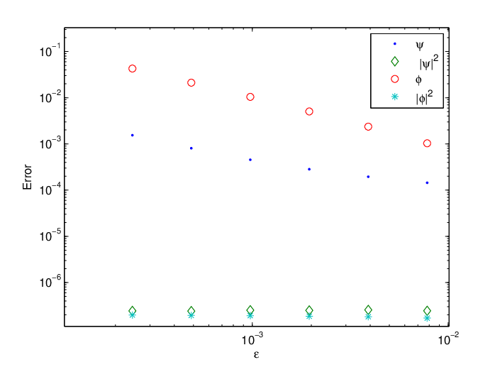
Refer to caption
Figure 7. Fix Δ\Delta t=0.005. For ε=1256\varepsilon=\frac{1}{256}, 1512\frac{1}{512}, 11024\frac{1}{1024}, 12048\frac{1}{2048}, 14096\frac{1}{4096}, Δ​x=ε8\Delta x=\frac{\varepsilon}{8}, respectively. The reference solution is computed with the same Δ​x\Delta x, but Δ​t=0.54​ε4\Delta t=\frac{0.54\varepsilon}{4}.

Example 3. In this example, we want to test the convergence in the spatial grid Δ​x\Delta x and in the time step Δ​t\Delta t. According to the previous analysis, the spatial oscillations of wavelength O⁡(ε)O(\varepsilon) need to be resolved. On the other hand, if the time oscillation with frequency O⁡(1/ε)O(1/\varepsilon) are resolved, one gets accurate approximation even of the wave functions itself (not only quadratic quantities of it). Unresolved time steps of order O⁡(1)O(1) can still give correct physical observable densities. More specifically, one expects second order convergence with respect time in both wave functions (and in the physical observables), and spectral convergence in the respective spatial variable.

Assume x,y∈[−π,π]x,y\in[-\pi,\pi] and let V⁡(x,y)=12​(x+y)2V(x,y)=\frac{1}{2}(x+y)^{2}. The initial conditions are of the WKB form,

ψinε​(x)=e−5​(x+0.1)2​ei​sin⁡x/ε,φinε​(y)=e−5​(y−0.1)2​ei​cos⁡y/ε.\psi^{\varepsilon}_{\rm in}(x)=e^{-5(x+0.1)^{2}}e^{i\sin{x}/\varepsilon},\quad\varphi^{\varepsilon}_{\rm in}(y)=e^{-5(y-0.1)^{2}}e^{i\cos{y}/\varepsilon}.

To test the spatial convergence, we take ε=1256\varepsilon=\frac{1}{256}, and the reference solution is computed by well resolved mesh Δ​x=2​π​ε64\Delta x=\frac{2\pi\varepsilon}{64}, Δ​t=0.4​ε16\Delta t=\frac{0.4\varepsilon}{16} until T=0.4T=0.4. Then, we compute with the same time step, but with difference spatial grids. The results are illustrated in Figure 8. We observe that, when Δ​x=O⁡(ε)\Delta x=O(\varepsilon), the error decays quickly to be negligibly small as Δ​x\Delta x decreases. However, when the spatial grids do not well resolve the ε\varepsilon-scale, the method would actually give solutions with O⁡(1)O(1) error.

Refer to caption
Figure 8. Fix ε=1256\varepsilon=\frac{1}{256} and Δ​t=0.4​ε16\Delta t=\frac{0.4\varepsilon}{16}. Take Δ​x=2​π​ε32\Delta x=\frac{2\pi\varepsilon}{32}, 2​π​ε16\frac{2\pi\varepsilon}{16}, 2​π​ε8\frac{2\pi\varepsilon}{8}, 2​π​ε4\frac{2\pi\varepsilon}{4}, 2​π​ε2\frac{2\pi\varepsilon}{2} and 2​π​ε1\frac{2\pi\varepsilon}{1} respectively. The reference solution is computed with the same Δ​t\Delta t, but Δ​x=2​π​ε64\Delta x=\frac{2\pi\varepsilon}{64}.

At last, to test the convergence in time, we take ε=11024\varepsilon=\frac{1}{1024}, and the reference solution is computed through a well resolved mesh with Δ​x=2​π​ε16\Delta x=\frac{2\pi\varepsilon}{16}, Δ​t=0.48192\Delta t=\frac{0.4}{8192} till T=0.4T=0.4. Then, we compute with the same spatial grids, but with different time steps. The results are illustrated in the Figure 9. We observe that the method is stable even if Δ​t≫ε\Delta t\gg\varepsilon. Moreover we get second order convergence in the wave functions as well as in the physical observable densities.

Refer to caption
Figure 9. Fix ε=11024\varepsilon=\frac{1}{1024} and Δ​x=2​π16\Delta x=\frac{2\pi}{16}. Take Δ​t=0.432\Delta t=\frac{0.4}{32}, 0.464\frac{0.4}{64}, 0.4128\frac{0.4}{128}, 0.4256\frac{0.4}{256}, 0.4512\frac{0.4}{512} and 0.41024\frac{0.4}{1024}, respectively. The reference solution is computed with the same Δ​x\Delta x, but Δ​t=0.48192\Delta t=\frac{0.4}{8192}.

7.2. SVSP2 method for the Ehrenfest equations

Now we solve the Ehrenfest equations (6.11) by the SVSP2 method. Assume x∈[−π,π]x\in[-\pi,\pi], and assume periodic boundary conditions for the electronic wave equation.

Example 4. In this example, we want to test if δ\delta-independent time steps can be taken to capture correct physical observables and the convergence in the time step which is expected to be of the second order. The potential is again V⁡(x,y)=12​(x+y)2V(x,y)=\frac{1}{2}(x+y)^{2} and the initial conditions are chosen to be

ψδ​(x,0)=e−5​(x+0.1)2​ei​sin⁡x/δ,y⁡(0)=0,η⁡(0)=0.1.\psi^{\delta}(x,0)=e^{-5(x+0.1)^{2}}e^{i\sin{x}/\delta},\quad y(0)=0,\quad\eta(0)=0.1.

First, we test whether δ\delta-independent Δ​t\Delta t can be taken to capture the correct physical observables. We solve the equations with resolved spatial grids, which means Δ​x=O⁡(δ)\Delta x=O(\delta). The numerical solutions with Δ​t=O⁡(δ)\Delta t=O(\delta) are used as the reference solutions. For δ=1/256\delta=1/256, 1/5121/512, 1/10241/1024, 1/20481/2048, 1/40961/4096, we fix Δ​t=0.464\Delta t=\frac{0.4}{64}, and compute until T=0.4T=0.4. The l2l^{2} norm of the error in wave functions, the error in position densities, and the error in the coordinates of the nucleus are calculated. We see in Figure 10 that the error in the wave functions increases as δ→0+\delta\rightarrow 0_{+}, but the errors in physical observables and in the classical coordinates do not change notably.

Refer to caption
Figure 10. Fix Δ​t=0.464\Delta t=\frac{0.4}{64}. For δ=1256\delta=\frac{1}{256}, 1512\frac{1}{512}, 11024\frac{1}{1024}, 12048\frac{1}{2048}, 14096\frac{1}{4096}, Δ​x=2​π​ε/16\Delta x=2\pi\varepsilon/16, respectively. The reference solution is computed with the same Δ​x\Delta x, but Δ​t=δ10\Delta t=\frac{\delta}{10}.

Next, we test the convergences with respect to the time step in the wave function, the physical observables and the classical coordinates. We take δ=11024\delta=\frac{1}{1024}, and the reference solution is computed by well resolved mesh Δ​x=2​π​ε16\Delta x=\frac{2\pi\varepsilon}{16}, Δ​t=0.48192\Delta t=\frac{0.4}{8192} till T=0.4T=0.4. Then, we compute with the same spatial grids, but with difference time steps. The results are illustrated in the Figure 11. We observe that, the method is stable even if Δ​t≫ε\Delta t\gg\varepsilon, and clearly, we get second order convergence in the wave functions, the physical observable densities and the classical coordinates.

Refer to caption
Figure 11. Fix δ=11024\delta=\frac{1}{1024} and Δ​x=2​π16\Delta x=\frac{2\pi}{16}. Take Δ​t=0.432\Delta t=\frac{0.4}{32}, 0.464\frac{0.4}{64}, 0.4128\frac{0.4}{128}, 0.4256\frac{0.4}{256}, 0.4512\frac{0.4}{512} and 0.41024\frac{0.4}{1024}, respectively. The reference solution is computed with the same Δ​x\Delta x, but Δ​t=0.48192\Delta t=\frac{0.4}{8192}.

References

  • [1] G. Aki, P. Markowich, and C. Sparber, Classical limit for semi-relativistic Hartree systems, J. Math. Phys. 49 (2008), no.10, 102110, 10 pp.
  • [2] W. Bao, S. Jin, and P. A. Markowich, Numerical study of time-splitting spectral discretizations of nonlinear Schrödinger equations in the semiclassical regimes, SIAM J. Sci. Comput. 25 (2003), no.1, 27–64.
  • [3] W. Bao, S. Jin, and P. A. Markowich, On Time-Splitting Spectral Approximations for the Schrödinger Equation in the Semi-classical Regime, J. Comput. Phys. 175 (2002), no.2, 487–524.
  • [4] F. Bornemann and C. Schütte, On the Singular Limit of the Quantum-Classical Molecular Dynamics Model, SIAM J. Appl. Math. 59 (1999) 1208–1224.
  • [5] F. Bornemann, P. Nettesheim, and C. Schütte, Quantum-classical Molecular Dynamics as an Approximation to Full Quantum Dynamics, J. Chem. Phys. 105 (1996), 1074–1083.
  • [6] T. Cazenave, Semilinear Schrödinger equations, Courant Lecture Notes in Mathematics vo. 10, New York University, 2003.
  • [7] K. Drukker, Basics of Surface Hopping in Mixed Quantum/Classical Simulations, J. Comput. Phys. 153 (1999), 225–272.
  • [8] I. Gasser and P. A. Markowich, Quantum hydrodynamics, Wigner transforms and the classical limit, Asymptotic Analysis 14 (1997), no. 2, 97–116.
  • [9] P. Gérard, P. Markowich, N. Mauser, and F. Poupaud, Homogenization Limits and Wigner transforms, Comm. Pure Appl. Math. 50 (1997), 323–379.
  • [10] R. B. Gerber, V. Buch, and M. A. Ratner, Time-dependent self-consistent field approximation for intramolecular energy transfer. I. Formulation and application to dissociation of van der Waals molecules, J. Chem. Phys. 77 (1982), 3022–3030.
  • [11] R. B. Gerber and M. A. Ratner,Mean-field models for molecular states and dynamics New developments, J. Phys. Chem. 92 (1988), 3252–3260.
  • [12] E. Hairer, C. Lubich, and G. Wanner, Geometric numerical integration: structure-preserving algorithms for ordinary differential equations, vo. 31, Springer, 2006.
  • [13] J. Hinze, MC-SCF. I. The multi-configurational self-consistent-field method, J. Chem. Phys. 59 (1973), 6424–6432.
  • [14] S. Jin, C. D. Levermore, and D. W. McLaughlin, The behavior of solutions of the NLS equation in the semi-classical limit, in Singular Limits of Dispersive Waves, in Singular limits of dispersive waves, Springer US (1994), 235–255.
  • [15] S. Jin, P. Markowich, and C. Sparber, Mathematical and computational methods for semi-classical Schrödinger equations, Acta Num. 20 (2011), 211–289.
  • [16] S. Jin and Z. Zhou, A semi-Lagrangian time splitting method for the Schro¨\ddot{\rm{o}}dinger equation with vector potentials, Comm. Inf. Syst. 13 (2013), no. 3, 247–289.
  • [17] P. A. Markowich, P. Pietra, and C. Pohl, Numerical approximation of quadratic observables of Schrödinger type equations in the semi-classical limit, Numer. Math. 81, (1999), 595–630.
  • [18] C. Klein, Fourth order time-stepping for low dispersion Korteweg-de Vries and nonlinear Schrödinger equations. Electronic Trans. Num. Anal. 29 (2008), 116–135.
  • [19] Z. Kotler, E. Neria, and A. Nitzan, Multiconfiguration time-dependent self-consistent field approximations in the numerical-solution of quantum dynamic problems, Comput. Phys. Comm. 63 (1991), 243–258.
  • [20] P.-L. Lions and T. Paul, Sur les measures de Wigner, Rev. Math. Iberoamericana 9 (1993), 553–618.
  • [21] P. Markowich and N. Mauser, The classical limit of a self-consistent quantum-Vlasov equation in 3-D, Math. Models Methods Appl. Sci. 3 (1993), no. 1, 109–124.
  • [22] H. Spohn and S. Teufel, Adiabatic Decoupling and Time-Dependent Born Oppenheimer Theory, Comm. Math. Phys. 224 (2001), issue 1, 113–132.
  • [23] C. Sparber, P. A. Markowich, and N. J. Mauser, Wigner functions versus WKB-methods in multivalued geometrical optics, Asymptotic Analysis 33 (2003), no. 2, 153–187.
  • [24] X. Sun and W. H. Miller, Mixed semi-classical classical approaches to the dynamics of complex molecular systems, J. Chem. Phys. 106 (1997), no.3, 916–927.
  • [25] E. Wigner, On the Quantum Correction for the Thermodynamic Equilibrium, Phys. Rev. 40 (1932), 749–759.