Model-based clustering of multivariate binary data with dimension reduction

Binary data are commonly observed and analyzed in many application fields: behavioral and social research, biosciences, document classification, and inference on binary images. For example, Ekholm et al. (2000) analyzed biomedical data including five unequally spaced binary self-assessment measurements of arthritis and obesity data on the presence or absence of obesity in five cohorts of children. Also, the binarized data of the MovieLens 100K and the Netflix dataset, which are popular datasets for collaborative filtering tasks, have been analyzed by Kozma et al. (2009). One of the purposes of analyzing binary data, as well as continuous data, is the partitioning of binary objects into several unpredetermined homogeneous groups (clusters). For clustering of multivariate data, it is quite important to know if some of the variables do not contribute much to the structure of clusters because the inclusion of redundant information can reduce the performance of the cluster analysis (Milligan, 1996). Also, a lower-dimensional (say two or three dimensional) representation of the cluster structure, based on the most significant information, is very useful for evaluating and interpreting the results of the cluster analysis.

Hence, what is needed is a procedure that constructs a low-dimensional representation of the multivariate binary data, such that the cluster structure in the data is maximally revealed. For this purpose, researchers often carry out a preliminary dimension reduction technique (e.g., Collins et al., 2002; Schein et al., 2003; Lee et al., 2010). Cluster analysis is then performed on the object scores on the first few principal components. Although it is easy to implement, this two-step sequential approach, also called the tandem approach, provides no assurance that the components extracted in the first step are optimal for the subsequent cluster analysis, because the two steps are implemented separately by optimizing a different loss function (Arabie and Hubert, 1994; DeSarbo et al., 1990; De Soete and Carroll, 1994; Vichi and Kiers, 2001; Timmerman et al., 2010; Yamamoto and Hwang, 2014). For multivariate continuous data, instead of the two-step tandem clustering procedure, several methods that simultaneously perform cluster analysis and dimension reduction have been proposed (De Soete and Carroll, 1994; Vichi and Kiers, 2001, Ghahramani and Hinton, 1997; Yoshida et al., 2004).

On the other hand, for multivariate binary data, a few methods can conduct the analysis for simultaneously obtaining a cluster structure and a subspace for the cluster structure. Patrikainen and Mannila (2004) have developed a subspace clustering method of binary data that can be used in high-dimensional settings. Bouguila (2010) has developed a clustering method for multivariate binary data with feature weighting that allows variable selection taking variables with large weights. Recently, Wu (2013) has proposed a penalized latent class model for clustering extremely large-scale discrete data. This method can be also considered a weighting method. Cagnone and Viroli (2012) have proposed a factor mixture analysis model for multivariate binary data, in which latent variables are distributed as a finite mixture of multivariate Gaussian distributions.

In this paper, we focus on the common subspace clustering in which a cluster structure is present in a low-dimensional space. As described above, Patrikainen and Mannila’s (2004) method allows for obtaining a cluster structure and a subspace for the cluster structure simultaneously. However, their method is rather cluster-specific subspace clustering. In addition, in the past few decades, because of technical advances in storing and processing data, we can obtain a large dataset that includes a large number of variables. Thus, we need to take into account such high-dimensional data. In a high-dimensional setting, weighting methods for high-dimensional data, such as those of Bouguila (2010) and Wu (2013), may be promising because variables that have lower weights are suggested for exclusion from the model. However, their methods do not provide explicit low-dimensional representation of the data, which is useful for evaluating and interpreting the cluster structure. Thus, in this paper, we propose a new method to simultaneously find a cluster structure of multivariate binary data and an optimal low-dimensional space for clustering. Furthermore, our proposed method can deal with high-dimensional data.

The remainder of this paper is structured as follows. In Section 2, we propose a new method to cluster multivariate binary data with dimension reduction. Section 3 describes an algorithm for the proposed optimization problem. Section 4 is devoted to studying the working of the clustering method using artificial and real data examples. Finally, we sum up our findings and set out directions for future expansion in Section 5.

Let $\tilde{\bm{y}}=(\tilde{y}_{1},\dots,\tilde{y}_{D})^{\prime}$ be a random vector of $D$ binary variables. Suppose there are $K$ latent (unobservable) classes in a population and let $\tilde{u}_{k}$, $k=1,\dots,K$, be an allocation variable that takes “1” if an observation belongs to class $k$, and “0” otherwise. We write $\tilde{\bm{u}}=(\tilde{u}_{1},\dots,\tilde{u}_{K})^{\prime}$. We assume that the allocation variable follows a multinomial distribution, i.e., the probability that $\tilde{\bm{u}}$ takes the value $\bm{u}=(u_{1},\dots,u_{K})^{\prime}$ is

$$f(\tilde{\bm{u}}=\bm{u})=\prod_{k=1}^{K}\xi_{k}^{u_{k}},$$

where $\xi_{k}=\Pr(\tilde{u}_{1}=0,\dots,\tilde{u}_{k}=1,\dots,\tilde{u}_{K}=0)$.

Given that an observation is in the $k$th latent class, the probability that the random vector $\tilde{\bm{y}}$ takes the value $\bm{y}=(y_{1},\dots,y_{D})^{\prime}$, where each $y_{d}$ takes $0$ or $1$, is represented as $\Pr(\tilde{\bm{y}}=\bm{y}\mid\tilde{u}_{k}=1)$. The unconditional probability of the response $\bm{y}$ when we do not know the latent class of the observation is

$$\Pr(\tilde{\bm{y}}=\bm{y})=\sum_{k=1}^{K}\xi_{k}\Pr(\tilde{\bm{y}}=\bm{y}\mid\tilde{u}_{k}=1).$$

(1)

Here, we need to specify how the probability $\Pr(\tilde{\bm{y}}=\bm{y}\mid\tilde{u}_{k}=1)$ depends on parameters. We postulate that, given the latent class to which an observation belongs, the responses on the binary variables are independent:

$$\Pr(\tilde{\bm{y}}=\bm{y}\mid\tilde{u}_{k}=1)=\prod_{d=1}^{D}\Pr(\tilde{y}_{d}\mid\tilde{u}_{k}=1).$$

(2)

This assumption of conditional independence has been widely used in latent class modeling in sociology (Collins and Lanza, 2010), and is directly analogous to the assumption in the factor analysis model that observed variables are conditionally independent given the factors (Aitkin et al., 1981).

Finally, to specify the model completely, we need to specify a set of parameters that define the conditional probability of $\tilde{\bm{y}}$, with the value of $\tilde{\bm{u}}$ given. Suppose that $\tilde{\bm{y}}_{1},\dots,\tilde{\bm{y}}_{N}$ are mutually independent random variables that have the same distribution as $\tilde{\bm{y}}$, and the entries of $\mathbf{Y}=(y_{nd})$ are those realizations. We assume that, given the class $k$, $\tilde{y}_{d}$ follows the Bernoulli distribution with success probability $\pi_{kd}$. For the traditional latent class analysis model (Aitkin et al., 1981), we consider a parameter vector $\bm{\theta}_{k}=(\theta_{k1},\dots,\theta_{kD})^{\prime}$, where $\theta_{kd}$ is the logit transformation of $\pi_{kd}$. We define the inverse logit transformation $\pi(\theta)=\{1+\exp(-\theta))\}^{-1}$. The success probabilities can be represented using the canonical parameters $\theta_{kd}$ as $\pi_{kd}=\pi(\theta_{kd})$. Let $\tilde{y}_{nd}$ be the $d$th element of $\tilde{\bm{y}}_{n}$. The individual data-generating probability given the class then becomes

	$\displaystyle\Pr(\tilde{y}_{nd}=y_{nd}\mid\tilde{u}_{k}=1)$	$\displaystyle=\Pr(\tilde{y}_{nd}=y_{nd}\mid\tilde{u}_{k}=1,\theta_{kd})$
		$\displaystyle=\pi(\theta_{kd})^{y_{nd}}\{1-\pi(\theta_{kd})\}^{1-y_{nd}}$
		$\displaystyle=\pi(q_{nd}\theta_{kd}),$

with $q_{nd}=2y_{nd}-1$ since $\pi(-\theta)=1-\pi(\theta)$. Then, these representations lead to the compact form of the log likelihood as

$$\sum_{n=1}^{N}\log\left(\sum_{k=1}^{K}\xi_{k}\prod_{d=1}^{D}\pi(q_{nd}\theta_{kd})\right).$$

We aim to obtain a low-dimensional representation of binary data in which the true cluster structure exists. Thus, we assume that canonical parameter $\theta_{kd}$ has a low-rank representation as follows:

$$\theta_{kd}=\mu_{d}+\bm{f}_{k}^{\prime}\bm{a}_{d},$$

(3)

where $\mu_{d}\in\mathbb{R}$, and for some positive integer $L$, $\bm{f}_{k}\in\mathbb{R}^{L}$ and $\bm{a}_{d}\in\mathbb{R}^{L}$. Here, $\mu_{d}$, $\bm{f}_{k}$, and $\bm{a}_{d}$ denote a centroid for the $d$th variable, a component score of the $k$th cluster, and a loading value for the $d$th variable, respectively. We write $\bm{\xi}=(\xi_{1},\dots,\xi_{K})^{\prime}$, $\bm{\mu}=(\mu_{1},\dots,\mu_{D})^{\prime}$, $\mathbf{F}=(\bm{f}_{1},\dots,\bm{f}_{K})^{\prime}$, and $\mathbf{A}=(\bm{a}_{1},\dots,\bm{a}_{D})^{\prime}$. To guarantee identifiability, we require that $\mathbf{F}$ has orthonormal columns. Then the log likelihood can be written as

$$\ell(\bm{\xi},\bm{\mu},\mathbf{F},\mathbf{A})=\sum_{n=1}^{N}\log\left(\sum_{k=1}^{K}\xi_{k}\prod_{d=1}^{D}\pi(q_{nd}(\mu_{d}+\bm{f}_{k}^{\prime}\bm{a}_{d}))\right).$$

(4)

Here, to deal with the high-dimensional problem, we assume that most of the elements of the true $\mathbf{A}$ are exactly zero. A sparse loading matrix implies variable selection in cluster analysis. That is, variables with non-zero loadings can be considered to contribute to a cluster structure in a low-dimensional space, whereas variables with zero loadings have no effect on the cluster structure. We propose to perform variable selection using the penalized likelihood with sparsity-inducing penalties. If $K=1$ and $\bm{f}_{k}$ is observable, Eq. (4) is the log likelihood for $D$ logistic regression models. This connection with logistic regression suggests the use of the $L_{1}$ penalty to obtain a sparse loading matrix, as in the Lasso regression (Tibshirani, 1996). Specifically, consider the penalty

$$P_{\lambda}(\mathbf{A})=\sum_{l=1}^{L}\lambda_{l}\|\check{\bm{a}}_{l}\|_{L_{1}}=\lambda_{1}\sum_{d=1}^{D}|a_{d1}|+\dots+\lambda_{L}\sum_{d=1}^{D}|a_{dL}|,$$

where $\check{\bm{a}}_{l}$ denotes the $l$th column of $\mathbf{A}$ and $\lambda_{l}$ is a regularization parameter. The choice of values for $\lambda_{l}$ will be discussed later. We obtain cluster components $\bm{\xi}$, $\bm{\mu}$, and $\mathbf{F}$ and a sparse loading matrix $\mathbf{A}$ by maximizing the following penalized log likelihood:

$$S(\bm{\xi},\bm{\mu},\mathbf{F},\mathbf{A})=\ell(\bm{\xi},\bm{\mu},\mathbf{F},\mathbf{A})-N\cdot P_{\lambda}(\mathbf{A}).$$

(5)

We call this procedure the clustering of binary data with reducing the dimensionality (CLUSBIRD). We can interpret penalized maximization as the device for generating a suitable optimization function, but not a realistic representation of the actual data-generating process. Thus, in this sense, the conditional independence given the latent class for obtaining the likelihood in Eq. (4) is assumed. A computational algorithm for solving the maximization problem is presented in the next section.

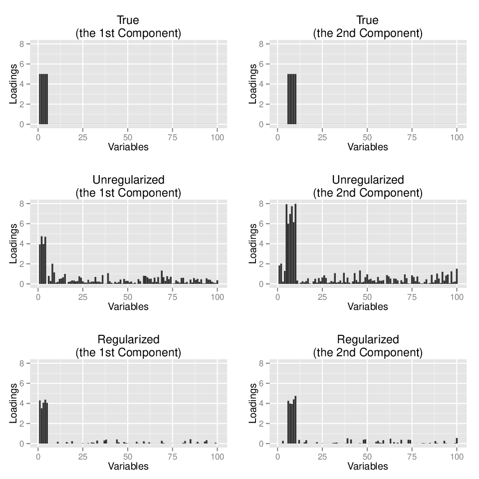The effectiveness of the introduction of sparsity is illustrated in Figure 1 using a rank-two model (i.e., $L=2$). The details of the setting will be presented in Section 4. While the regularized model can recover the original loading vector efficiently under the sparsity assumption, the unregularized model gives more noisy results. In the context of the ordinary factor analysis model, a sparse structure for the loading matrix provides an easy interpretation of the result, whereas it is difficult to interpret the relation between variables and factors if the loading matrix has no sparse structure. Browne (2001) provides an excellent overview of the sparsity and rotation techniques which aim to obtain a sparse structure. In addition, Hirose and Yamamoto (2014) discuss the sparsity problem in the factor analysis model. Similar to the ordinary factor analysis model, noisy loading values may lead to difficulty in the interpretation of the result in our model. Thus, for the proposed model, sparse loading values offer an advantage.

As is often the case, we apply the EM algorithm (Dempster et al., 1977) to solve the maximization problem (5). Let $\mathbf{U}=(u_{nk})$ be $N$ realizations of mutually independent random variable $\tilde{\bm{u}}$. In addition, denote the conditional probability (2) by $p_{k}(\bm{y}\mid\bm{\theta}_{k})$. Then, the complete-data likelihood can be written as follows:

$$L^{C}(\mathbf{Y},\mathbf{U}\mid\bm{\xi},\bm{\mu},\mathbf{F},\mathbf{A})=\prod_{n=1}^{N}\left\{\prod_{k=1}^{K}p_{k}(\bm{y}_{n}\mid\bm{\theta}_{k})^{u_{k}}\prod_{k=1}^{K}\xi_{k}^{u_{k}}\right\}.$$

As described in the previous section, we aim to obtain the sparse loading matrix $\mathbf{A}$; therefore, the penalty term for sparsity should be introduced. Thus, the complete-data log-likelihood with the penalty is

$\displaystyle\ell^{C}(\mathbf{Y},\mathbf{U}$

$\displaystyle\mid\bm{\xi},\bm{\mu},\mathbf{F},\mathbf{A})=\sum_{n=1}^{N}\sum_{k=1}^{K}u_{nk}\log p_{k}(\bm{y}_{n}\mid\bm{\theta}_{k})+\sum_{n=1}^{N}\sum_{k=1}^{K}u_{nk}\log\xi_{k}-N\cdot P_{\lambda}(\mathbf{A}).$

(6)

The EM algorithm consists of a step maximizing the conditional expectation of the complete-data log-likelihood function (6) given the observable data $\mathbf{Y}$ and a set of parameters, $\{\bm{\xi}^{(t)},\bm{\mu}^{(t)},\mathbf{F}^{(t)},\mathbf{A}^{(t)}\}$. Here, $\bm{\xi}^{(t)}$ denotes the value of $\bm{\xi}$ at the $t$th step in the algorithm, and this notation is applied to other parameters. From the above formulation, we can see that the penalized complete-data log-likelihood (6) is a linear function with respect to values of $u_{nk}$. Thus, to obtain the conditional expected value of $\ell^{C}$, we only have to replace $u_{nk}$ with its conditional expectation,

	$\displaystyle u_{nk}^{*}$	$\displaystyle:=E\left[u_{nk}\mid\mathbf{Y};\bm{\xi}^{(t)},\bm{\mu}^{(t)},\mathbf{F}^{(t)},\mathbf{A}^{(t)}\right]$
		$\displaystyle=\frac{\xi_{k}^{(t)}p_{k}(\bm{y}_{n}\mid\bm{\theta_{k}}^{(t)})}{\sum_{k=1}^{K}\xi_{k}^{(t)}p_{k}(\bm{y}_{n}\mid\bm{\theta_{k}}^{(t)})},$		(7)

where $\bm{\theta}_{k}^{(t)}=(\theta_{k1}^{(t)},\dots,\theta_{kD}^{(t)})^{\prime}$, $k=1,\dots,K$, is obtained through Eq. (3) using $\{\bm{\xi}^{(t)},\bm{\mu}^{(t)},\mathbf{F}^{(t)},\mathbf{A}^{(t)}\}$. Thus, the conditional expectation of the complete-data log-likelihood is as follows:

	$\displaystyle Q(\bm{\xi},\bm{\mu},\mathbf{F},\mathbf{A}$	$\displaystyle\mid\bm{\xi}^{(t)},\bm{\mu}^{(t)},\mathbf{F}^{(t)},\mathbf{A}^{(t)})$
		$\displaystyle=E\left[\ell^{C}\mid\mathbf{Y};\bm{\xi}^{(t)},\bm{\mu}^{(t)},\mathbf{F}^{(t)},\mathbf{A}^{(t)}\right]$
		$\displaystyle=\sum_{n=1}^{N}\sum_{k=1}^{K}u_{nk}^{*}\log p_{k}(\bm{y}_{n}\mid\bm{\theta}_{k})+\sum_{n=1}^{N}\sum_{k=1}^{K}u_{nk}^{*}\log\xi_{k}-N\cdot P_{\lambda}(\mathbf{A}).$

In the M-step of the EM algorithm, we consider the following maximization problem

$$(\hat{\bm{\xi}},\hat{\bm{\mu}},\hat{\mathbf{F}},\hat{\mathbf{A}})=\mathop{\rm arg~max}\limits_{\bm{\xi},\bm{\mu},\mathbf{F},\mathbf{A}}Q(\bm{\xi},\bm{\mu},\mathbf{F},\mathbf{A}\mid\bm{\xi}^{(t)},\bm{\mu}^{(t)},\mathbf{F}^{(t)},\mathbf{A}^{(t)}).$$

(8)

Same as the usual mixture models, the estimate of $\bm{\xi}$ can be obtained by

$$\hat{\xi}_{k}=N^{-1}\sum_{n=1}^{N}u_{nk}^{*},\ \ \text{for $k=1,\dots,K-1$},$$

(9)

and $\hat{\xi}_{K}=1-\sum_{k=1}^{K-1}\hat{\xi}_{k}$.

Given the estimate of $\bm{\xi}$, the maximization problem in (8) with respect to $\bm{\mu}$, $\mathbf{F}$, and $\mathbf{A}$ is equivalent to the minimization of the following function:

$$g(\bm{\mu},\mathbf{F},\mathbf{A})=-\sum_{n=1}^{N}\sum_{k=1}^{K}u_{nk}^{*}\log p_{k}(\bm{y}_{n}\mid\bm{\theta}_{k})+N\cdot P_{\lambda}(\mathbf{A}).$$

(10)

Here, the function $g$ in (10) is non-quadratic. Then, instead of directly dealing with the non-quadratic function $g$, we minimize a surrogate function, called the majorizing function (Hunter and Lange, 2004), to solve the minimization problem of a quadratic function. In the majorization algorithm, a suitably defined quadratic upper bound of (10) is minimized, which provides optimal values for the actual function $m$. A function $h(x\mid y)$ is said to majorize a function $m(x)$ at $y$ if

$$h(x\mid y)\geq m(x)\ \ \ \text{for all $x$}\ \ \ \text{and}\ \ \ h(y\mid y)=m(y).$$

In the geometrical view, the function surface $h(x\mid y)$ lies above the function $m(x)$ and is tangent to it at the point $y$; therefore $h(x\mid y)$ becomes an upper bound of $m(x)$. To minimize $m(x)$, the majorization algorithm decreases the objective function $m(x)$ in each step and is guaranteed to converge to a local minimum of $m(x)$. When applying the majorization algorithm, the majorizing function $h(x\mid y)$ is chosen so that it is easier to minimize than the original objective function $m(x)$. The study by Hunter and Lange (2004) can be referred for an introductory description of the majorization algorithm.

To find a suitable majorizing function of (10), we consider the first term of (10). Note that, for a given point $y$,

$$-\log\pi(x)\leq-\log\pi(y)-\{1-\pi(y)\}(x-y)+\frac{1}{8}(x-y)^{2},$$

(11)

and the equality holds when $x=y$ (Jaakkola and Jordan, 2000; De Leeuw, 2006). This equation provides quadratic upper bounds for the first term of (10) at the tangent point $y$. Thus we can apply the majorization algorithm for our problem.

We now present details of the majorization algorithm via the upper bound of $-\log\pi(x)$ in (11). By completing the square, Eq. (11) can be rewritten as

$$-\log\pi(x)\leq-\log\pi(y)+\frac{1}{8}\left[x-y-4\left\{1-\pi(y)\right\}\right]^{2}.$$

(12)

Substituting $x$ and $y$ with $q_{nd}\theta_{kd}$ and $q_{nd}\theta_{kd}^{(t)}$, respectively in (12) and using $q_{nd}=\pm 1$, we obtain

$$-\log\pi(q_{nd}\theta_{kd})\leq-\log\pi(q_{nd}\theta_{kd}^{(t)})+\frac{1}{8}(\theta_{kd}-z_{nkd}^{(t)})^{2},$$

(13)

where

$$z_{nkd}^{(t)}=\theta_{kd}^{(t)}+4q_{nd}\left\{1-\pi(q_{nd}\theta_{kd}^{(t)})\right\}.$$

Thus, we obtain the following quadratic upper bound of the first term of (10):

$$\frac{1}{8}\sum_{n=1}^{N}\sum_{k=1}^{K}u_{nk}^{*}\sum_{d=1}^{D}(\theta_{kd}-z_{nkd}^{(t)})^{2}.$$

(14)

Eq. (14) then yields the following upper bound (up to a constant) of the criterion function $g(\bm{\mu},\mathbf{F},\mathbf{A})$ defined in (10):

	$\displaystyle h(\bm{\mu},$	$\displaystyle\mathbf{F},\mathbf{A}\mid\bm{\mu}^{(t)},\mathbf{F}^{(t)},\mathbf{A}^{(t)})$
		$\displaystyle=\frac{1}{8}\sum_{n=1}^{N}\sum_{k=1}^{K}u_{nk}^{*}\|\bm{z}_{nk}^{(t)}-(\bm{\mu}+\mathbf{A}\bm{f}_{k})\|^{2}+N\cdot P_{\lambda}(\mathbf{A}),$		(15)

where $\bm{z}_{nk}^{(t)}=(z_{nk1}^{(t)},\dots,z_{nkD}^{(t)})^{\prime}$.

The majorizing function given in (15) is quadratic in each of $\bm{\mu}$, $\mathbf{F}$, and $\mathbf{A}$ when the other two are fixed, and thus alternating minimization of (15) with respect to $\bm{\mu}$ and $\mathbf{A}$ has closed-form solutions. We now drop the subscript $(t)$ for notational convenience. For fixed $\mathbf{F}$ and $\mathbf{A}$, set $\bar{z}_{kd}=N_{k}^{-1}\sum_{n=1}^{N}u_{nk}^{*}z_{nkd}$ where $N_{k}=\sum_{n=1}^{N}u_{nk}^{*}$, and write $\bar{\bm{z}}_{k}=(\bar{z}_{k1},\dots,\bar{z}_{kD})^{\prime}$. Then the optimal $\hat{\bm{\mu}}$ is given by

	$\displaystyle\hat{\bm{\mu}}$	$\displaystyle=\mathop{\rm arg~min}\limits_{\bm{\mu}}\sum_{n=1}^{N}\sum_{k=1}^{K}u_{nk}^{*}\|\bm{z}_{nk}-(\bm{\mu}+\mathbf{A}\bm{f}_{k})\|^{2}$
		$\displaystyle=N^{-1}\sum_{k=1}^{K}N_{k}(\bar{\bm{z}}_{k}-\mathbf{A}\bm{f}_{k}).$		(16)

Optimization of $\mathbf{F}$ requires a numerical procedure because of its orthonormality. To update $\mathbf{F}$ for fixed $\bm{\mu}$ and $\mathbf{A}$, we apply the gradient projection (GP) algorithm with the orthonormal constraint (Jennrich, 2001, 2002). The only problem specific thing required for the GP algorithm is the gradient of (15) viewed as a function of $\mathbf{F}$. Let $\bar{z}_{kd}^{*}=N_{k}^{-1}\sum_{n=1}^{N}u_{nk}(z_{nkd}-\mu_{d})$, and write $\bar{\mathbf{Z}}^{*}=(\bar{z}_{kd}^{*})$. Furthermore, let $\mathbf{N}$ be a $K\times K$ diagonal matrix where the $k$th diagonal element is $N_{k}$. Then, the gradient of $h$ at $\mathbf{F}$ is given as follows:

$$\mathbf{\Gamma}=\frac{\partial h}{\partial\mathbf{F}}=\frac{1}{4}\mathbf{N}(\mathbf{F}\mathbf{A}^{\prime}-\bar{\mathbf{Z}}^{*})\mathbf{A}.$$

(17)

Using $\mathbf{\Gamma}$ as the gradient in the GP algorithm with orthonormal constraint, we obtain the optimal $\hat{\mathbf{F}}$.

Finally, for fixed $\bm{\mu}$ and $\mathbf{F}$, the $dl$th element $a_{dl}$ of $\mathbf{A}$ is updated by solving the minimization problem in (15) directly. Let $v_{dl}=\sum_{n=1}^{N}\sum_{k=1}^{K}u_{nk}^{*}(z_{nkd}-\mu_{d})f_{kl}$ and $w_{ll^{\prime}}=\sum_{k}^{K}N_{k}f_{kl}f_{kl^{\prime}}$. Then, up to a constant, the loss function with respect to $\mathbf{A}$ can be written as

$\displaystyle h^{\prime}(\mathbf{A})$

$\displaystyle=\frac{1}{8}\sum_{d=1}^{D}\sum_{l=1}^{L}\sum_{l^{\prime}=1}^{L}w_{ll^{\prime}}a_{dl}a_{dl^{\prime}}-\frac{1}{4}\sum_{d=1}^{D}\sum_{l=1}^{L}v_{dl}a_{dl}+N\sum_{l=1}^{L}\lambda_{l}\sum_{d=1}^{D}|a_{dl}|.$

(18)

Let $s_{dl}=\sign(a_{dl})$ for $a_{dl}\neq 0$, and $s_{dl}\in[-1,1]$ for $a_{dl}=0$. Thus, the subdifferential $\partial h^{\prime}_{dl}(\mathbf{A})$ of $h^{\prime}(\mathbf{A})$ at $a_{dl}$ is as follows:

$$\partial h^{\prime}_{dl}(\mathbf{A})=\left\{\frac{1}{4}\sum_{l^{\prime}=1}^{L}w_{ll^{\prime}}a_{dl^{\prime}}-\frac{1}{4}v_{dl}+N\lambda_{l}s_{dl}\right\}.$$

(19)

Then, the optimal $\hat{a}_{dl}$ can be obtained by

$$\hat{a}_{dl}=\frac{1}{w_{ll}}\sign(c_{dl})\max(0,|c_{dl}|-4N\lambda_{l}),$$

(20)

where $c_{dl}=-\sum_{l^{\prime}\neq l}a_{dl^{\prime}}+v_{dl}$.

The procedure of the proposed optimization algorithm is summarized as follows:

1. STEP1.

   Set $t=1$ and initial values of $\bm{\xi}^{(1)}$, $\bm{\mu}^{(1)}$, $\mathbf{F}^{(1)}$, and $\mathbf{A}^{(1)}$.

2. STEP2.

   Calculate the conditional expectation of $u_{nk}$ using (7).

3. STEP3.

   Update $\bm{\xi}$ using (9) and set $\bm{\xi}^{(t+1)}=\hat{\bm{\xi}}$.

4. STEP4.

   Update $\bm{\mu}$ using (16) and set $\bm{\mu}^{(t+1)}=\hat{\bm{\mu}}$.

5. STEP5.

   Update $\mathbf{F}$ by the GP algorithm with the gradient $\mathbf{\Gamma}$ in (17) and set $\mathbf{F}^{(t+1)}=\hat{\mathbf{F}}$.

6. STEP6.

   Update $\mathbf{A}$ using (20) and set $\mathbf{A}^{(t+1)}=\hat{\mathbf{A}}$.

7. STEP7.

   Increase the value of $t$ by 1 and repeat STEP2-6 until the penalized log-likelihood (5) converges.

Prior to applying the above algorithm, the value of the regularization parameters, $\bm{\lambda}=(\lambda_{1},\dots,\lambda_{L})^{\prime}$, should be determined. In regression analysis, the degree of freedom for the shrinkage method (Zou et al, 2007; Hirose et al., 2013) may be used for selecting the model selection criteria. In this paper, we choose $\bm{\lambda}$ by minimizing the following Bayesian information criterion (BIC):

$$\text{BIC}(\lambda)=-2\ell(\bm{\xi},\bm{\mu},\mathbf{F},\mathbf{A})+(\log N)\df(\bm{\lambda}),$$

(21)

where $\df(\bm{\lambda})$ is the number of nonzero parameters for fixed $K$ and $L$. The degree of freedom $\df(\bm{\lambda})$ used in Eq. (21) is defined as $\df(\bm{\lambda})=K+D+KL+|\mathbf{A}|_{\bm{\lambda}}$, where $K$ and $D$ are the length of the vector $\bm{\xi}$ and $\bm{\mu}$, respectively, $KL$ is the total number of elements of $\mathbf{F}$, and $|\mathbf{A}|_{\bm{\lambda}}$ is the number of nonzero elements of $\mathbf{A}$ when the regularization parameter is $\bm{\lambda}$. In the following sections, we use the above BIC to choose $\bm{\lambda}$ in the proposed method. In addition, although different parameters can be used for different component loading vectors, we consider using only a single regularization parameter $\lambda$ for all loadings.

In this paper, we proposed a new procedure, called CLUSBIRD, for simultaneously finding the optimal cluster structure for multivariate binary objects and finding the subspace to represent the cluster structure. The proposed method can provide the weight for each binary variable, which indicates the contribution of the variable to the cluster structure. In general, tandem analysis for clustering objects with dimension reduction is likely to fail in finding the cluster structure. In fact, our numerical examples demonstrate the inability of tandem analysis to detect the cluster structure and subspace for the structure. Those examples also show that our proposed method can provide a better cluster structure than tandem analysis. Furthermore, from the examples, we found that our procedure can work well for data that had a mildly larger number of variables than the sample size.

The proposed model can be considered an extension of the ordinary latent class analysis (LCA) (Aitkin et al., 1981). However, the ordinary LCA cannot provide loading values for variables and a low-dimensional structure. Also, LCA may not provide an appropriate estimation with the moderately high-dimensional dataset we used in the numerical examples. From this point of view, the proposed method can provide useful insight for researchers.

The proposed method can be extended to deal with various problems. For example, it is useful for the proposed model to deal with categorical variables, not just binary variables. In addition, the ordinary LCA model is ready for multi-group analysis, the analysis with covariates, and analysis of repeated measures data (Collins and Lanza, 2009). Using the formulation of LCA, the proposed model can also contain those features. These could be interesting topics for further research.

References

- Aitkin (1981) Aitkin Aitkin, M., Anderson, D., and Hinde, J. (1981). Statistical modeling of data on teaching styles. Journal of the Royal Statistical Society, Series A, 144, 419–461.
- Arabie (1994) Arabie Arabie, P. and Hubert, L. (1994). Cluster analysis in marketting research. In Bagozzi, R.P., editor, Advanced methods of marketing research (pp.160–189). Blackwell, Oxford.
- Bache (2013) Bache, K. and Lichman, M. (2013). UCI Machine Learning Repository [http://archive.ics.uci.edu/ml]. Irvine, CA: University of California, School of Information and Computer Science. Accessed Apr. 24, 2014.
- Bouguila (2010) Bouguila Bouguila, N. (2010). On multivariate binary data clustering and feature weighting. Computational Statistics & Data Analysis, 54, 120–134.
- Browne (2001) Browne, M.W. (2001). An overview of analytic rotation in exploratory factor analysis. Multivariate Behavioral Research, 36, 111–150.
- Cagnone (2012) Cagnone Cagnone, S. and Viroli, C. (2012). A factor mixture analysis model for multivariate binary data. Statistical Modelling, 12, 257–277.
- Collins (2002) Collins Collins, M., Dasgupta, S., and Schapire, R.E. (2002). A generalization of principal component analysis to the exponential family. In Advanced in Neural Information Processing System (T.G. Dietterich, S. Becker, and Z. Ghahramani, eds.), 14, 617–642. MIT Press, Cambridge, MA.
- Collins (2010) Collins Collins, L.M. and Lanza, S.T. (2010). Latent class and latent transition analysis with applications in the social, behavioral, and health sciences. John Wiley & Sons, Inc., New Jersey.
- deLeeuw (2006) deLeeuw De Leeuw, J. (2006). Principal component analysis of binary data by iterated singular value decomposition. Computational Statistics & Data Analysis, 50, 21–39.
- De Soete et al. (1994) De Soete and Carroll De Soete, G. and Carroll, J.D. (1994). K-means clustering in a low-dimensional Euclidean space. In Diday, E. and Lechevallier, Y. and Schader, M. and Bertrand, P. and Burtschy, B. (Eds.) New Approaches in Classification and Data Analysis (pp. 212-219). Springer, Heidelberg
- Dempster (1977) Dempster Dempster, N.M., Laird, A.P., and Rubin, D.B. (1977). Maximum likelihood from incomplete data via the EM algorithm (with discussion), Journal of the Royal Statistical Society B, 39, 1–38.
- DeSarbo (1990) DeSarbo DeSarbo, W.S., Jedidi, K., Cool, K., and Schendel, D. (1990). Simultaneous multidimensional unfolding and cluster analysis: An investigation of strategic groups. Marketing Letters, 2, 129–146.
- Ekholm (2000) Ekholm, A., McDonald, J.W., and Smith, P.W.F. (2000). Association models for a multivariate binary response. Biometrics, 56, 712–718.
- Ewens (1995) Ewens, W.J. and Spielman, R.S. (1995). The transmission/disequilibrium test: History, subdivision, and admixture. The American Journal of Human Genetics, 57, 455–464.
- Ghahramani (1997) Ghahramani Ghahramani, Z. and Hilton, G.E. (1997). The EM algorithm for mixture of factor analyzers. Technical Report CRG-TR-96-1, Department of Computer Science, University of Toronto, Canada.
- Hao (2004) Hao, K., Li, C., Rosenow, C., and Wong, W.H. (2004). Detect and adjust for population stratification in population-based association study using genomic control markers: An application of Affymetrix Genechip® Human Mapping 10K array. European Journal of Human Genetics, 12, 1001–1006.
- Hirose (2013) Hirose, K., Tateishi, S., and Konishi, S. (2013). Tuning parameter selection in sparse regression modeling. Computational Statistics & Data Analysis, 59, 28–40.
- Hirose (2014) Hirose, K., and Yamamoto, M. (2014). Sparse estimation via nonconcave penalized likelihood in a factor analysis model. Statistics and Computing, in press.
- Hunter (2004) Hunter Hunter, D.R. and Lange, K. (2004). A tutorial on MM algorithms. The American Statistician, 58, 30–37.
- Jaakkola (2000) Jaakkola Jaakkola, T.S. and Jordan, M.I. (2000). Bayesian parameter estimation via variational methods. Statistics and Computing, 10, 25–37.
- Jennrich (2001) Jennrich Jennrich, R.I. (2001). A simple general procedure for orthogonal rotation. Psychometrika, 66, 289–306.
- Jennrich (2002) Jennrich Jennrich, R.I. (2002). A simple general procedure for oblique rotation. Psychometrika, 67, 7–20.
- Juan (2004) Vidal Juan, A. and Vidal, E. (2004). Bernoulli mixture models for binary images. Proceedings of the ICPR 2004.
- Kozma (2009) Kozma, L., Ilin, A., and Raiko, T. (2009). Binary principal component analysis in the Netflix collaborative filtering task. Proceedings of 2009 IEEE International Workshop on Machine Learning for Signal Processing.
- Lee (2010) Lee Lee, S. and Huang, J.Z. and Hu, J. (2010). Sparse logistic principal components analysis for binary data. The Annals of Applied Statistics, 4, 1579–1601.
- Milligan (1996) Milligan, G.W. (1996). Clustering validation: Results and implications for applied analysis. In: Arabie, P., Hubert, L.J., De Soete, G. (Eds.), Clustering and Classification. World Scientific Publishing, River Edge, pp. 341–375.
- Patrilainen (2004) Patrikainen Patrikainen, A. and Mannila, H. (2004). Subspace clustering of high-dimensional binary data - a probabilistic approach. In Workshop on Clustering High Dimensional Data and its Applications, SIAM International Conference on Data Mining. 57–65.
- Purcell (2007) Purcell, S., Neale, B., Todd-Brown, K., Thomas, L., Ferreira, M.A.R., Bender, D., Maller, J., Sklar, P., de Bakker, P.I.W., Daly, M.J., and Sham, P.C. (2007). PLINK: a toolset for whole-genome association and population-based linkage analysis. American Journal of Human Genetics, 81.
- Schein (2003) Schein Schein, A.I., Saul, L.K., and Ungar, L.H. (2003). A generalized linear model for principal component analysis of binary data. In Proceedings of the Ninth International Workshop on Artificial Intelligence and Statistics (C.M. Bishop and B.J. Frey, eds.), 38, 14–21. Key West, FL.
- Tamhane (2009) Tamhane Tamhane, A.C., Qiu, D., and Ankenman, B.E. (2010). A parametric mixture model for clustering multivariate binary data. Statistical Analysis and Data Mining, 3, 3–19.
- Hapmap (2005) The International HapMap Consortium. (2005). A haplotype map of the human genome. Nature, 437, 1299–1320.
- Tibshirani (1996) Tibshirani Tibshirani, R.J. (1996). Regression shrinkage and selection via the lasso. Journal of the Royal Statistical Society, Series B, 58, 267–288.
- Timmerman (2010) Timmerman Timmerman, M.E., Ceulemans, E., Kiers, H.A.L., and Vichi, M. (2010). Factorial and reduced k-means reconsidered. Computational Statistics & Data Analysis, 54, 1858–1871.
- Vichi et al. (2001) Vichi and Kiers Vichi, M. and Kiers, H.A.L. (2001). Factorial k-means analysis for two-way data. Computational Statistics & Data Analysis, 37, 49–64.
- Wu (2013) Wu, B. (2013). Sparse cluster analysis of large-scale discrete variables with application to single nucleotide polymorphism data. Journal of Applied Statistics, 40, 358–367.
- Yamamoto and Hwang (2014) Yamamoto, M. and Hwang, H. (2014). A general formulation of cluster analysis with dimension reduction and subspace separation. Behaviormetrika, 41, 115–129.
- Yoshida (2004) Yoshida Yoshida, R., Higuchi, T., and Imoto, S. (2004). A mixed factors model for dimension reduction and extraction of a group structure in gene expression data. Proceedings of the 2004 IEEE Computational Systems Bioinformatics Conference, 161–172.
- Zou (2007) Zou, H., Hastie, T., and Tibshirani, R. (2007). On the degrees of freedom of the lasso. The Annals of Statistics, 35, 2173–2192.