跳到论文正文
W Papers独立论文阅读器 arXiv:1406.3620 论文正文 计算阅读时间 · 0%
引用这篇论文根据当前论文元数据生成,正式投稿前建议核对。


License: arXiv.org perpetual non-exclusive license
arXiv:1406.3620v2 [math-ph] 01 Oct 2019

Singularities of the eigenvalue functions for first order symmetric symbols on rank two vector bundles over surfaces

Carlos Valero Valdes
Departamento de Matematicas
Universidad de Guanajuato
Guanajuato, México
Date: 01 Oct 2019
Abstract.

For a rank two bundle FF over a surface XX, we study the set of singularities ℳσ\mathcal{\mathcal{M}}_{\sigma} of the eigenvalue functions of symmetric symbols σ\sigma associated to first order differential operators on FF. We prove that the existence of these singularities follows from topological considerations. We define deg⁡(ℳσ)\deg(\mathcal{M}_{\sigma}) (the degree of ℳσ\mathcal{\mathcal{M}}_{\sigma}) and show that it can be used to “count” the number of directions at which special optical phenomena occur. For the case when F=T​XF=TX we compute a formula for deg⁡(ℳσ)\deg(\mathcal{\mathcal{M}}_{\sigma}) in terms of the Euler characteristics of XX and 𝒩σ\mathcal{N}_{\sigma}, where 𝒩σ⊂X\mathcal{N}_{\sigma}\subset X is a manifold with boundary associated to σ\sigma.

1. Introduction

Refer to caption
(a) Upon entering a bi-axial crystal along one of its optical axes, a light beam refracts as a slanted cone and then emerges as a cylinder.
Refer to caption
(b) Fresnel surface associated to a bi-axial crystal. This surface has four conical singularities, which account for the phenomenon of conical refraction.
Figure 1.1. Conical refraction

On the 22nd of October 1832, in the “Third Supplement to an Essay on the Theory of Systems of Rays”, William R. Hamilton predicted the phenomenon of conical refraction for bi-axial crystals based on the existence of conical singularities in its Fresnel surface (see Figure 1.1). The existence of this phenomenon has been applied to diverse fields, like optical trapping, free-space optical communications, polarization metrology, super-resolution imaging, two-photon polymerization, and lasers (see [11]).

The propagation of electromagnetic waves in a homogeneous and an-isotropic medium can be modeled by Maxwell’s equations (see [2, pg. 678])

(1.1) ∂E∂t−ϵ−1​(∇×B)\displaystyle\frac{\partial E}{\partial t}-\epsilon^{-1}(\nabla\times B) =0,\displaystyle=0,
(1.2) ∂B∂t+∇×E\displaystyle\frac{\partial B}{\partial t}+\nabla\times E =0,\displaystyle=0,

and

(1.3) ∇⋅(ϵ​E)=∇⋅B=0.\nabla\cdot(\epsilon E)=\nabla\cdot B=0.

In the above formulas we have assumed that the speed of light is equal to 11 and that ϵ\epsilon is a 3×33\times 3 positive definite symmetric matrix (known as the dielectric tensor). If for E0,B0∈ℝ3E_{0},B_{0}\in\mathbb{R}^{3} and (ξ,τ)∈(ℝ3×ℝ)∗(\xi,\tau)\in(\mathbb{R}^{3}\times\mathbb{R})^{*} we consider fields that move along planar waves, i.e

E⁡(x,t)\displaystyle E(x,t) =E0​exp⁡(i⁡(ξ⋅x−τ​t)),\displaystyle=E_{0}\exp(i(\xi\cdot x-\tau t)),
B⁡(x,t)\displaystyle B(x,t) =B0​exp⁡(i⁡(ξ⋅x−τ​t)),\displaystyle=B_{0}\exp(i(\xi\cdot x-\tau t)),

by substitution into equations 1.1 and 1.2 we obtain

(1.4) (τ​I−σϵ​(ξ))​(E0B0)=0,(\tau I-\sigma_{\epsilon}(\xi))\left(\begin{array}[]{c}E_{0}\\ B_{0}\end{array}\right)=0,

where II is the 6×66\times 6 identity matrix,

σϵ​(ξ)=(0−ϵ−1​P​(ξ)P⁡(ξ)0)\sigma_{\epsilon}(\xi)=\left(\begin{array}[]{cc}0&-\epsilon^{-1}P(\xi)\\ P(\xi)&0\end{array}\right)

and

P⁡(ξ)=(0−ξ3ξ2ξ30−ξ1−ξ2ξ10).P(\xi)=\left(\begin{array}[]{ccc}0&-\xi_{3}&\xi_{2}\\ \xi_{3}&0&-\xi_{1}\\ -\xi_{2}&\xi_{1}&0\end{array}\right).

To find non-trivial solutions of Equation 1.4 we need to solve the characteristic equation

(1.5) det(τ​I−σϵ​(ξ))=0.\det(\tau I-\sigma_{\epsilon}(\xi))=0.

The matrix σϵ​(ξ)\sigma_{\epsilon}(\xi) has 00 as an eigenvalue of multiplicity 22 and the other four eigenvalues are of the form −λϵ,1​(ξ),λϵ,1​(ξ),−λϵ,2​(ξ)-\lambda_{\epsilon,1}(\xi),\lambda_{\epsilon,1}(\xi),-\lambda_{\epsilon,2}(\xi) and λϵ,2​(ξ)\lambda_{\epsilon,2}(\xi), where the functions λϵ,1\lambda_{\epsilon,1} and λϵ,2\lambda_{\epsilon,2} are homogenous of degree one. The Fresnel surface associated to ϵ\epsilon is the set

ℱϵ=ℱϵ1∪ℱϵ2\mathcal{F}_{\epsilon}=\mathcal{F}_{\epsilon}^{1}\cup\mathcal{F}_{\epsilon}^{2}

where

ℱϵi={ξ∈(ℝ3)∗|λϵ,i(OPENξ)=1}.\mathcal{F}_{\epsilon}^{i}=\{\xi\in(\mathbb{R}^{3})^{*}|\lambda_{\epsilon,i}(\text{$\xi)=1$}\}.

The sets ℱϵ1\mathcal{F}_{\text{$\epsilon$}}^{1} and ℱϵ2\mathcal{F}_{\epsilon}^{2} correspond to the inner and outer sheets of the surface shown in Figure 1.1b. The existence of the four conical singularities in ℱϵ\mathcal{F}_{\epsilon} follows from the fact that λϵ,1\lambda_{\epsilon,1} and λϵ,2\lambda_{\epsilon,2}, when restricted to the sphere S2={ξ∈(ℝ3)∗|<ξ,ξ>=1}S^{2}=\{\xi\in(\mathbb{R}^{3})^{*}|<\xi,\xi>=1\}, are non-smooth at the multiplicity set

ℳϵ={ξ∈S2|λϵ,1​(ξ)=λϵ,2​(ξ)}.\mathcal{M}_{\epsilon}=\{\xi\in S^{2}|\lambda_{\epsilon,1}(\xi)=\lambda_{\epsilon,2}(\xi)\}.

1.1. First order hyperbolic differential operators with constant coefficients

We can study the problem discussed above for Maxwell’s equations in a more general setting. Consider the first order linear partial differential equation

(1.6) HL​u=0​ for ​u:ℝn×ℝ→ℝk,H_{L}u=0\hbox{\,\,\,for\,\,\,}u:\mathbb{R}^{n}\times\mathbb{R}\rightarrow\mathbb{R}^{k},

where

(1.7) HL=∂∂t​I+L​ for ​L=∑i=1nAi​∂∂xi​ for ​Ai∈Mk×k​(ℝ),H_{L}=\frac{\partial}{\partial t}I+L\hbox{\,\,for\,\,}L=\sum_{i=1}^{n}A_{i}\frac{\partial}{\partial x_{i}}\hbox{\,\,for\,\,}A_{i}\in M_{k\times k}(\mathbb{R}),

and II is the identity k×kk\times k matrix.

Remark.

Maxwell’s equations 1.1 and 1.2 can be written in the form 1.6 for an operator LL with appropriate coefficients A1,A2,A3∈M6×6​(ℝ)A_{1},A_{2},A_{3}\in M_{6\times 6}(\mathbb{R}).

If for u0u_{0} in ℝk\mathbb{R}^{k} we substitute fields of the form u=u0​exp⁡(ξ⋅x−τ​t)u=u_{0}\exp(\xi\cdot x-\tau t) into 1.6 we obtain the equation

(1.8) (τ​I−σL​(ξ))​u0=0(\tau I-\sigma_{L}(\xi))u_{0}=0

where

σL​(ξ1,…,ξn)=∑i=1nAi​ξi​ for ​ξ=(ξ1,…,ξn).\sigma_{L}(\xi_{1},\ldots,\xi_{n})=\sum_{i=1}^{n}A_{i}\xi_{i}\hbox{\,\,\,for\,\,\,}\xi=(\xi_{1},\ldots,\xi_{n}).

To solve 1.8 we need to solve the characteristic equation det(σ⁡(ξ)−τ​I)=0\det(\sigma(\xi)-\tau I)=0. As in the case of Maxwells equations, we are interested in the points ξ∈Sn−1\xi\in S^{n-1} at which σL​(ξ)\sigma_{L}(\xi) has multiple eigenvalues. This condition has been studied by P. Lax in [8], F. John in [6] and B.A. Khesin in [7]. In [10] Friedland, Robbin and Sylvester elegantly reduced this problem to Adams’ celebrated theorem on linearly independent vector fields on the sphere. The problem is also related to the 1929 celebrated von Neumann–Wigner theorem on the non-crossing rule (see [5]).

1.2. First order hyperbolic differential operators on vector bundles

The above ideas can be generalized even further to the case of first order hyperbolic linear partial differential equations on bundles. More concretely, consider a Riemannian manifold XX with metric <,>.<,>. The cotangent bundle T∗​XT^{*}X inherits a metric from that of T​XTX by letting the map v↦<v,⋅>v\mapsto<v,\cdot> be an isometry . Consider a vector bundle FF over XX, a linear differential operator L:C∞​(F)→C∞​(F)L:C^{\infty}(F)\rightarrow C^{\infty}(F) of order one, and the equation

(1.9) HL​u=0​ where ​HL=∂∂t+LH_{L}u=0\hbox{\,\,where\,\,}H_{L}=\frac{\partial}{\partial t}+L

where u:X×ℝ→Fu:X\times\mathbb{R}\rightarrow F is a time dependent section of FF. We are interested in high frequency solutions of 1.9. More concretely, for a section u0:X→Fu_{0}:X\rightarrow F and a phase function φ:X×ℝ→ℝ\varphi:X\times\mathbb{R}\rightarrow\mathbb{R} we consider oscillatory sections of the form

us​(x,t)=u0​ei​s​φ​(x,t).u_{s}(x,t)=u_{0}e^{is\varphi(x,t)}.

By substitution into equation 1.9 and letting s↦∞s\mapsto\infty we obtain (for the details of the derivation this formula the reader is referred to books on asymptotic methods like [14, 12, 4] )

(1.10) (∂φ∂t​(x,t)​I+σ⁡(dx​φ​(x,t)))​u0=0,\left(\frac{\partial\varphi}{\partial t}(x,t)I+\sigma(d_{x}\varphi(x,t))\right)u_{0}=0,

where I:F→FI:F\rightarrow F is the identity morphism and σ:T∗​X→End​(F)\sigma:T^{*}X\rightarrow\hbox{End}(F) is the principal symbol of L.L. Since we are assuming that LL is a differential operator of degree one, for every x∈Xx\in X we have that σ\sigma is a linear map from Tx∗​XT^{*}_{x}X to End​(Fx)\hbox{End}(F_{x}). A necessary condition for 1.10 to hold is that φ\varphi satisfies the non-linear partial differential equation of first order, know as the characteristic equation, given by

(1.11) det(∂φ∂t​(x,t)​I+σ⁡(dx​φ​(x,t)))=0.\det\left(\frac{\partial\varphi}{\partial t}(x,t)I+\sigma(d_{x}\varphi(x,t))\right)=0.

This equation can be interpreted as follows. For a particle x:ℝ→Xx:\mathbb{R}\rightarrow X traveling on a wave front defined by the equation

φ⁡(x⁡(t),t)=constant\varphi(x(t),t)=\hbox{constant}

we have that

∂φ∂t​(x,t)=−<∇xφ​(x,t),x˙>,\frac{\partial\varphi}{\partial t}(x,t)=-<\nabla_{x}\varphi(x,t),\dot{x}>,

so formula 1.11 becomes

det(⟨n⁡(x,t),x˙⟩​I−σ⁡(n♭​(x,t)))=0\det\left(\left\langle n(x,t),\dot{x}\right\rangle I-\sigma\left(n^{\flat}(x,t)\right)\right)=0

for

n⁡(x,t)=∇xφ​(x,t)|∇xφ​(x,t)|​ and ​n♭​(x,t)=dx​φ​(x,t)|dx​φ​(x,t)|.n(x,t)=\frac{\nabla_{x}\varphi(x,t)}{|\nabla_{x}\varphi(x,t)|}\hbox{\,\,and\,\,}n^{\flat}(x,t)=\frac{d_{x}\varphi(x,t)}{|d_{x}\varphi(x,t)|}.

We conclude that if a particle moves in a wave front

Yt={x∈X|φ⁡(x,t)=constant}Y_{t}=\{x\in X|\varphi(x,t)=\hbox{constant}\}

then the component of its velocity normal to the wave front must be an eigenvalue of σ​(n♭​(x,t))\sigma(n^{\flat}(x,t)). Hence, for a unitary co-vector ξ∈Tx∗​X\xi\in T_{x}^{*}X the eigenvalues of σ⁡(ξ)\sigma(\xi) are the allowable normal velocities of particles moving along wave fronts whose tangent spaces at xx is the kernel of ξ\xi. If λσ,i:T∗​X→ℝ\lambda_{\sigma,i}:T^{*}X\rightarrow\mathbb{R} are the eigenvalues of σ\sigma (ordered as λσ,1≤⋯≤λσ,k\lambda_{\sigma,1}\leq\text{$\cdots$}\leq\lambda_{\sigma,k}) then we are interested in the non-zero covectors ξ∈T∗​X\xi\in T^{*}X at which λσ,i​(ξ)=λσ,j​(ξ)\lambda_{\sigma,i}(\xi)=\lambda_{\sigma,j}(\xi) for some i<ji<j.

1.3. Symmetric symbols and characteristic functions

In this paper we will only be interested in the case where the symbol σ\sigma is a symmetric symbol, i.e we will assume that for a metric <,>F<,>_{F} in FF we have that for all x∈Xx\in X and ξ∈Tx∗​X\xi\in T^{*}_{x}X the following holds

<σ⁡(ξ)​v,w>F=<v,σ⁡(ξ)​w>F​ for all ​v,w∈Fx.<\sigma(\xi)v,w>_{F}=<v,\sigma(\xi)w>_{F}\hbox{\,\,for\,all\,}v,w\in F_{x}.

If we denote the bundle of symmetric endomorphisms of FF by S2​F\hbox{S}^{2}F, then σ\sigma is a morphism of the form σ:T∗​X→S2​F\sigma:T^{*}X\rightarrow\hbox{S}^{2}F. Symmetric symbols appear in diverse physical problems derived from variational principles (see [1, Ch. 8]). If λσ,1​(ξ),…,λσ,k​(ξ)\lambda_{\sigma,1}(\xi),\ldots,\lambda_{\sigma,k}(\xi) are the eigenvalues of σ⁡(ξ)\sigma(\xi) then the characteristic equation 1.11 is equivalent to the Hamilton-Jacobi equations

(1.12) ∂φ∂t​(x,t)+λσ,i​(dx​φ​(x,t))=0​ for ​i=1,…,k,\frac{\partial\varphi}{\partial t}(x,t)+\lambda_{\sigma,i}(d_{x}\varphi(x,t))=0\hbox{\,for\,\,}i=1,\ldots,k,

where kk is the rank of FF. We will refer to the functions λσ,i:T∗​X→ℝ\lambda_{\sigma,i}:T^{*}X\rightarrow\mathbb{R} as the eigenvalue functions of the symbol σ\sigma. For hyperbolic partial differential equations which correspond to generic non-homogeneous media the existence of non-smooth points of the eigenvalue functions account for a phenomena known as wave transformation, in which longitudinal waves convert into transversal waves or vice-versa (see [1, Ch. 8] and [3]). Hence, it is important to find methods for detecting points at which the eigenvalue functions of a symbol become non-smooth.

1.4. Plan of the paper

For the rest of the paper we will assume that XX is a Riemannian compact, connected and oriented surface, and FF an SO​(2)\hbox{SO}(2) vector bundle of rank 22 over XX. For a first order differential operator acting on FF and having a symmetric symbol σ:T∗​X→S2​F\sigma:T^{*}X\rightarrow\hbox{S}^{2}F, we are interested in studying the multiplicity set

ℳσ={ξ∈S⁡(T∗​X)|λσ,1​(ξ)=λσ,2​(ξ)}.\mathcal{M}_{\sigma}=\{\xi\in S(T^{*}X)|\lambda_{\sigma,1}(\xi)=\lambda_{\sigma,2}(\xi)\}.

The reason for restricting our study of ℳσ\mathcal{M}_{\sigma} to XX and FF as above is that in this case we can prove many interesting properties of ℳσ\mathcal{M}_{\sigma}, which we hope will pave the way and motivate the relevant questions for the more general cases. Our main results can be summarized as follows:

  • •

    We will show that for symbols σ\sigma in general position the multiplicity set ℳσ\mathcal{M}_{\sigma} is a 11-dimensional sub-manifold of S⁡(T∗​X)S(T^{*}X) which can be characterized as the set of points at which the eigenvalue functions λσ,1\lambda_{\sigma,1} and λσ,2\lambda_{\sigma,2} are non-smooth (see Proposition 3).

  • •

    We will give a topological obstruction for ℳσ\mathcal{M}_{\sigma} to be empty. More concretely, we will show that if e⁡(T​X)e(TX) and e⁡(F)e(F) are the Euler classes of T​XTX and FF, then e⁡(T​X)−2​e​(F)≠0e(TX)-2e(F)\not=0 in H2​(X,ℝ)H^{2}(X,\mathbb{R}) implies that ℳσ≠∅\mathcal{M}_{\sigma}\not=\emptyset (Theorem 4). In particular, if F=T​XF=TX and the genus of XX is not 00 then ℳσ\mathcal{M}_{\sigma} must always be non-empty ( 4).

  • •

    We will show that for symbols σ\sigma in general position the set ℳσ\mathcal{M}_{\sigma} is the intersection of S⁡(T∗​X)S(T^{*}X) with a real line bundle 𝒦σ⊂T∗​X\mathcal{K}_{\sigma}\subset T^{*}X over one dimensional sub-manifold of 𝒮σ\mathcal{S}_{\sigma} of XX (Theorem 8 and Corollary 5). This will allow us to define the integer deg⁡(ℳσ)∈ℤ\deg(\mathcal{M}_{\sigma})\in\mathbb{Z} as the number of times that 𝒦σ\mathcal{K}_{\sigma} turns as we move along 𝒮σ\mathcal{S}_{\sigma}. We will provide a physical interpretation of this number to motivate its relevance.

  • •

    We will prove that when F=T​XF=TX a symbol σ\sigma has two associated sections v:X→Fv:X\rightarrow F and w:X→F⊗ℂF⊗ℂFw:X\rightarrow F\otimes_{\mathbb{C}}F\otimes_{\mathbb{C}}F (Theorem 13 and Corollary 14) such that

    𝒮σ={x∈X||w⁡(x)/v⁡(x)|=1}\mathcal{S}_{\sigma}=\{x\in X||w(x)/v(x)|=1\}

    and

    ℳσ=⋃x∈𝒮σ{z♭∈Tx∗​X|z∈Tx​X​ and ​z2=w⁡(x)v⁡(x)}.\mathcal{M}_{\sigma}=\bigcup_{x\in\mathcal{S}_{\sigma}}\left\{z^{\flat}\in T^{*}_{x}X|z\in T_{x}X\hbox{\,\,and\,\,}z^{2}=\frac{w(x)}{v(x)}\right\}.

    From this result we will obtain the following formula (see Theorem 22)

    deg⁡(ℳσ)=3​χ​(X)−2​χ​(𝒩σ),\deg(\mathcal{M}_{\sigma})=3\chi(X)-2\chi(\mathcal{N}_{\sigma}),

    where

    𝒩σ={x∈X||w⁡(x)/v⁡(x)|≤1},\mathcal{N}_{\sigma}=\{x\in X||w(x)/v(x)|\leq 1\},

    and χ⁡(X)\chi(X) and χ⁡(𝒩σ)\chi(\mathcal{N}_{\sigma}) are the Euler characteristics of XX and 𝒩σ\mathcal{N}_{\sigma}, respectively.

  • •

    We conclude the paper with the construction of some explicit examples of symbols on the plane (the only non-compact case considered) and the sphere, and use the formula in Theorem 22 to compute deg⁡(ℳσ)\deg(\mathcal{M}_{\sigma}) for these examples.

2. Symbols and Their Multiplicities

2.1. Preliminaries

From now on and for rest of the paper we will assume that FF is Riemannian orientable real vector bundle of rank 22, over an oriented Riemannian surface XX that is compact and connected. To distinguish the metrics in T​XTX and FF we will denote them by <,><,> and <,>F<,>_{F}, respectively. The metric in T​XTX induces isomorphism maps ♭:T​X→T∗​X\flat:TX\rightarrow T^{*}X and ♯:T∗​X→T​X\sharp:T^{*}X\rightarrow TX, such that for v,w∈Tx​Xv,w\in T_{x}X and ξ∈Tx∗​X\xi\in T^{*}_{x}X we have that

v♭​(w)=<v,w>​ and ​ξ​(w)=<ξ♯,w>.v^{\flat}(w)=<v,w>\hbox{\,\,and\,\,\,}\xi(w)=<\xi^{\sharp},w>.

The metric in T​XTX induces a metric T∗​XT^{*}X by letting

<ξ,η>=<ξ♯,η♯>.<\xi,\eta>=<\xi^{\sharp},\eta^{\sharp}>.

Observe that we are using the same notation for the metrics in T∗​XT^{*}X and T​XTX.

Let E1E_{1} and E2E_{2} be vector bundles over XX with projection maps π1\pi_{1} and π2\pi_{2}. A section s:X→Hom​(E1,E2)s:X\rightarrow\hbox{Hom}(E_{1},E_{2}) can be seen as a bundle morphism σs:E1→E2\sigma_{s}:E_{1}\rightarrow E_{2} given by

σs​(v)=s⁡(x)​v​ for ​x=π1​(v).\sigma_{s}(v)=s(x)v\hbox{\,\,for\,\,}x=\pi_{1}(v).

Similarly, a bundle morphism σ:E1→E2\sigma:E_{1}\rightarrow E_{2} can be seen as a sections sσ:X→Hom​(E1,E2)s_{\sigma}:X\rightarrow\hbox{Hom}(E_{1},E_{2}) given by

sσ​(x)​v=σ⁡(v)​ for ​v∈π1−1​(x).s_{\sigma}(x)v=\sigma(v)\hbox{\,\,for\,\,}v\in\pi_{1}^{-1}(x).

2.2. Symmetric symbols

Motivated by the discussion in the introduction, we introduce our basic objects of study.

Definition 1.

A symmetric symbol on the bundle F→XF\rightarrow X is a smooth bundle morphism σ:T∗​X→S2​F\sigma:T^{*}X\rightarrow\hbox{S}^{2}F.

From now on we will refer to a symmetric symbol simply as a symbol; since we will not be working with non-symmetric ones. Given that a symbol σ\sigma is a morphism of vector bundles, it is completely determined by the values it take on the sphere bundle

S⁡(T∗​X)={ξ∈T∗​X|<ξ,ξ>=1}.S(T^{*}X)=\{\xi\in T^{*}X|<\xi,\xi>=1\}.

The bundle S2​F\hbox{S}^{2}F has a natural Riemannian metric given by

g⁡(A,B)=12​tr​(A∘B)​ for all ​x∈X​ and ​A,B∈S2​Fx.g(A,B)=\frac{1}{2}\hbox{tr}(A\circ B)\hbox{\,\,for\,all\,\,}x\in X\hbox{\,and\,}A,B\in\hbox{S}^{2}F_{x}.

This metric induces a norm function on S2​F\hbox{S}^{2}F; which for an element A∈S2​FA\in\hbox{S}^{2}F we will denote by ‖A‖||A||. If we let

σ0=σ−12​tr​(σ)​I\sigma_{0}=\sigma-\frac{1}{2}\hbox{tr}(\sigma)I

be the traceless part of σ\sigma, the eigenvalue functions λσ,1,λσ,2:T∗​X→ℝ\lambda_{\sigma,1},\lambda_{\sigma,2}:T^{*}X\rightarrow\mathbb{R} of σ\sigma are given by

(2.1) λσ,1​(ξ)\displaystyle\lambda_{\sigma,1}(\xi) =\displaystyle= 12​tr​(σ⁡(ξ))−‖σ0​(ξ)‖,\displaystyle\frac{1}{2}\hbox{tr}(\sigma(\xi))-||\sigma_{0}(\xi)||,
(2.2) λσ,2​(ξ)\displaystyle\lambda_{\sigma,2}(\xi) =\displaystyle= 12​tr​(σ⁡(ξ))+‖σ0​(ξ)‖.\displaystyle\frac{1}{2}\hbox{tr}(\sigma(\xi))+||\sigma_{0}(\xi)||.
Refer to caption
(a)
Refer to caption
(b)
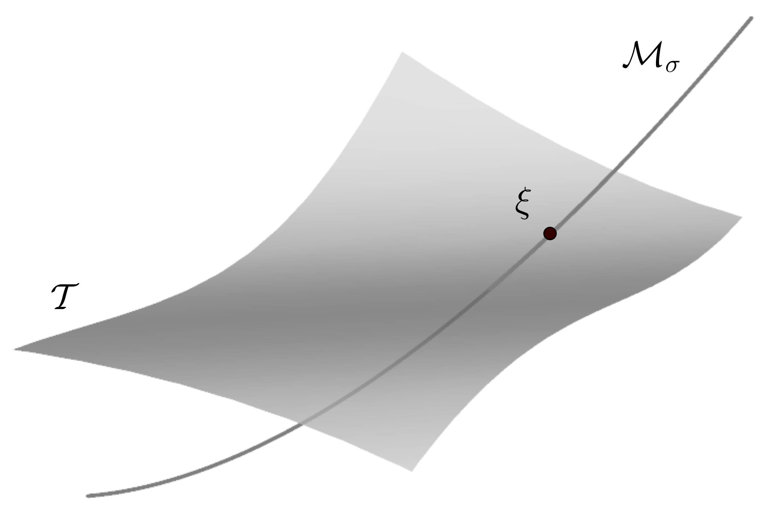
Figure 2.1. Conical singularities of the eigenvalue functions λσ,1\lambda_{\sigma,1} and λσ,2\lambda_{\sigma,2} of a symbol σ\sigma. On the left we show the multiplicity set ℳσ\mathcal{M}_{\sigma} and a transversal sub-manifold 𝒯\mathcal{T} to it at ξ∈ℳσ\xi\in\mathcal{M}_{\sigma}. On the right we show the graphs near ξ\xi of λσ,1|𝒯\lambda_{\sigma,1}|\mathcal{T} (lower cone) and λσ,2|𝒯\lambda_{\sigma,2}|\mathcal{T} (upper cone).
Definition 2.

The multiplicity set of a symbol σ\sigma is the set

ℳσ={ξ∈S⁡(T∗​X)|λσ,1​(ξ)=λσ,2​(ξ)}.\mathcal{M}_{\sigma}=\{\xi\in S(T^{*}X)|\lambda_{\sigma,1}(\xi)=\lambda_{\sigma,2}(\xi)\}.

From formulas 2.1 and 2.2 we have that

ℳσ={ξ∈S⁡(T∗​X)|σ0​(ξ)=0}.\mathcal{M}_{\sigma}=\{\xi\in S(T^{*}X)|\sigma_{0}(\xi)=0\}.

Let S02​F\hbox{S}_{0}^{2}F stand for the bundle of traceless elements in S2​F\hbox{S}^{2}F. If σ0|S⁡(T∗​X)\sigma_{0}|S(T^{*}X) is transversal to the 0-section of S02​F\hbox{S}_{0}^{2}F then ℳσ\mathcal{M}_{\sigma} is 1-dimensional sub-manifold of S⁡(T∗​X)S(T^{*}X). The following result shows that, for a symbol σ\sigma in general position, the set ℳσ\mathcal{M}_{\sigma} can be described as the set of elements in S⁡(T∗​X)S(T^{*}X) at which λσ,1|S⁡(T∗​X)\lambda_{\sigma,1}|S(T^{*}X) and λσ,2|S⁡(T∗​X)\lambda_{\sigma,2}|S(T^{*}X) are non-smooth (see Figure 2.1).

Proposition 3.

Consider a symbol σ\sigma and let σ0\sigma_{0} be its traceless part. If σ0|S⁡(T∗​X)\sigma_{0}|S(T^{*}X) is transversal to the zero section of S02​F\hbox{S}_{0}^{2}F then

ℳσ=sing​(λσ,1|S⁡(T∗​X))=sing​(λσ,2|S⁡(T∗​X)),\mathcal{M}_{\sigma}=\hbox{sing}(\lambda_{\sigma,1}|S(T^{*}X))=\hbox{sing}(\lambda_{\sigma,2}|S(T^{*}X)),

where for a function f:S⁡(T∗​X)→ℝf:S(T^{*}X)\rightarrow\mathbb{R} we have defined

sing​(f)={ξ∈S⁡(T∗​X)|f​ is non-smooth at ​ξ}.\hbox{sing}(f)=\{\xi\in S(T^{*}X)|f\hbox{\,\,is\,non-smooth\,at\,\,}\xi\}.
Proof.

By formulas 2.1 and 2.2 it is enough to show that the map f:S⁡(T∗​X)→ℝf:S(T^{*}X)\rightarrow\mathbb{R} given by

f⁡(ξ)=‖σ0​(ξ)‖f(\xi)=||\sigma_{0}(\xi)||

is non-smooth at ℳσ\mathcal{M}_{\sigma} and only on this set. The function ff is smooth in S⁡(T∗​X)−ℳσS(T^{*}X)-\mathcal{M}_{\sigma} since σ0\sigma_{0} is smooth and the norm function is smooth away from the 00-section of S02​F\hbox{S}_{0}^{2}F. We will now prove that ff is non-smooth at ℳσ\mathcal{M}_{\sigma}. The proof is local: consider an open set U⊂XU\subset X where we can find ortho-normal sections v,w:U→Fv,w:U\rightarrow F. We can then write

f⁡(ξ)=|(a⁡(ξ),b⁡(ξ))|​ for ξ∈S⁡(T∗​X|U),f(\xi)=|(a(\xi),b(\xi))|\text{{\,\,for\,\,}$\xi\in S(T^{*}X|U)$},

where

a⁡(ξ)\displaystyle a(\xi) =<σ0​(ξ)​v​(ξ),v⁡(ξ)>F,\displaystyle=<\sigma_{0}(\xi)v(\xi),v(\xi)>_{F},
b⁡(ξ)\displaystyle b(\xi) =<σ0​(ξ)​v​(ξ),w⁡(ξ)>F,\displaystyle=<\sigma_{0}(\xi)v(\xi),w(\xi)>_{F},

and

|(a,b)|=a2+b2.|(a,b)|=\sqrt{a^{2}+b^{2}}.

If we define ℳσ|U=ℳσ∩S⁡(T∗​X|UCLOSE\mathcal{M}_{\sigma}|U=\mathcal{M}_{\sigma}\cap S(T^{*}X|U) then

ℳσ|U={ξ∈S⁡(T∗​X|U)|(a⁡(ξ),b⁡(ξ))=(0,0)}.\mathcal{M}_{\sigma}|U=\{\xi\in S(T^{*}X|U)|(a(\xi),b(\xi))=(0,0)\}.

From the transversality assumptions we have that the linear functionals d​a​(ξ)da(\xi) and d​b​(ξ)db(\xi) are linearly independent, and

Tξ​ℳσ=ker⁡(d​a​(ξ))∩ker⁡(d​b​(ξ))​ for ​ξ∈ℳσ|U.T_{\xi}\mathcal{M}_{\sigma}=\ker(da(\xi))\cap\ker(db(\xi))\text{{\,\,for\,\,\,}}\xi\in\mathcal{M}_{\sigma}|U.

For ξ∈ℳσ\xi\in\mathcal{M}_{\sigma} consider any vector η∈Tξ​S​(T∗​X|U)\eta\in T_{\xi}S(T^{*}X|U) not in Tξ​ℳσT_{\xi}\mathcal{M}_{\sigma} and a curve α=α⁡(t)\alpha=\alpha(t) with α⁡(0)=ξ\alpha(0)=\xi and α˙​(0)=η\dot{\alpha}(0)=\eta. We have that

f⁡(α⁡(t))−f⁡(α⁡(0))t={|(a⁡(α⁡(t)),b⁡(α⁡(t))CLOSEt|t>0,−|(a⁡(α⁡(t)),b⁡(α⁡(t))CLOSEt|t<0.\frac{f(\alpha(t))-f(\alpha(0))}{t}=\begin{cases}\left|\frac{(a(\alpha(t)),b(\alpha(t))}{t}\right|&t>0,\\ -\left|\frac{(a(\alpha(t)),b(\alpha(t))}{t}\right|&t<0.\end{cases}

Hence

limt↦0+f⁡(α⁡(t))−f⁡(α⁡(0))t=|(d​a​(ξ)​η,d​b​(ξ)​η)|\lim_{t\mapsto 0^{+}}\frac{f(\alpha(t))-f(\alpha(0))}{t}=|(da(\xi)\eta,db(\xi)\eta)|

and

limt↦0−f⁡(α⁡(t))−f⁡(α⁡(0))t=−|(d​a​(ξ)​η,d​b​(ξ)​η)|.\lim_{t\mapsto 0^{-}}\frac{f(\alpha(t))-f(\alpha(0))}{t}=-|(da(\xi)\eta,db(\xi)\eta)|.

Since η∉Tξ​ℳσ\eta\not\in T_{\xi}\mathcal{M}_{\sigma} we have that |(d​a​(ξ)​η,d​b​(ξ)​η)|≠0|(da(\xi)\eta,db(\xi)\eta)|\not=0 and we conclude that ff is not differentiable at ξ\xi. ∎

2.3. Obstruction theory for the multiplicity set

We will now find topological obstructions for the set ℳσ\mathcal{M}_{\sigma} to be empty.

Theorem 4.

Consider a symbol σ:T∗​X→S2​F\sigma:T^{*}X\rightarrow\hbox{S}^{2}F and let e⁡(F),e⁡(T​X)∈H2​(X,ℝ)e(F),e(TX)\in H^{2}(X,\mathbb{R}) denote the Euler classes of FF and T​XTX, respectively. If e⁡(T​X)−2​e​(F)≠0e(TX)-2e(F)\not=0 in H2​(X,ℝ)H^{2}(X,\mathbb{R}) then ℳσ≠∅\mathcal{M}_{\sigma}\not=\emptyset.

Proof.

Consider a rotation matrix

Rθ=(cos⁡(θ)−sin⁡(θ)sin⁡(θ)cos⁡(θ))∈SO​(2)R_{\theta}=\left(\begin{array}[]{cc}\cos(\theta)&-\sin(\theta)\\ \sin(\theta)&\cos(\theta)\end{array}\right)\in\hbox{SO}(2)

and

A=(abb−a)∈S02​ℝ2.A=\left(\begin{array}[]{cc}a&b\\ b&-a\end{array}\right)\in\hbox{S}_{0}^{2}\mathbb{R}^{2}.

It easy to see that

Rθ​A​RθT=(pqq−p),R_{\theta}AR_{\theta}^{T}=\left(\begin{array}[]{cc}p&q\\ q&-p\end{array}\right),

where

(pq)=(cos⁡(2​θ)−sin⁡(2​θ)sin⁡(2​θ)cos⁡(2​θ))​(ab).\left(\begin{array}[]{c}p\\ q\end{array}\right)=\left(\begin{array}[]{cc}\cos(2\theta)&-\sin(2\theta)\\ \sin(2\theta)&\cos(2\theta)\end{array}\right)\left(\begin{array}[]{c}a\\ b\end{array}\right).

Since the transition functions of the bundle S02​F\hbox{S}_{0}^{2}F are the same as those of the bundle F⊗ℂFF\otimes_{\mathbb{C}}F, these bundles must be isomorphic. If ℳσ\mathcal{M}_{\sigma} were empty then we would have that σ0​(ξ)≠0\sigma_{0}(\xi)\not=0 for all ξ∈S⁡(T∗​X)\xi\in S(T^{*}X), which means that σ0\sigma_{0} is an isomorphism between T∗​XT^{*}X and S02​F\hbox{S}_{0}^{2}F. We conclude that T​XTX and F⊗ℂFF\otimes_{\mathbb{C}}F must be isomorphic and hence

e⁡(T​X)=e⁡(F⊗ℂF)=2​e​(F),e(TX)=e(F\otimes_{\mathbb{C}}F)=2e(F),

which contradicts the hypothesis of the theorem. Hence ℳσ≠∅\mathcal{M}_{\sigma}\not=\emptyset. ∎

Corollary 5.

If the genus of XX is different from one then the multiplicity set of any symbol σ:T∗​X→S2​(T​X)\sigma:T^{*}X\rightarrow\hbox{S}^{2}(TX) must be non-empty.

Proof.

This follows from the previous Proposition and the fact that

∫X(e⁡(T​X)−2​e​(T​X))=2​(g−1)≠0,\int_{X}(e(TX)-2e(TX))=2(g-1)\not=0,

where gg is the genus of XX. ∎

2.4. The singular set and the kernel bundle

In this section we will see that ℳσ\mathcal{M}_{\sigma} (when non-empty) is generically the intersection of S⁡(T∗​X)S(T^{*}X) with a line bundle 𝒦σ⊂T∗​X\mathcal{K}_{\sigma}\subset T^{*}X defined over a one dimensional sub-manifold 𝒮σ\mathcal{S}_{\sigma} of XX. Recall that a symbol σ:T∗​X→S2​F\sigma:T^{*}X\rightarrow\hbox{S}^{2}F can be seen as a section sσs_{\sigma} of Hom​(T∗​X,S2​F)\hbox{Hom}(T^{*}X,\hbox{S}^{2}F).

Definition 6.

The singular set 𝒮σ\mathcal{S}_{\sigma} and the kernel bundle 𝒦σ\mathcal{K}_{\sigma} of a symbol σ\sigma are the sets defined by

𝒮σ\displaystyle\mathcal{S}_{\sigma} =\displaystyle= {x∈X|dim(ker⁡(sσ0​(x)))>0},\displaystyle\left\{x\in X|\dim\left(\ker(s_{\sigma_{0}}(x))\right)>0\right\},
𝒦σ\displaystyle\mathcal{K}_{\sigma} =\displaystyle= ⋃x∈Sσker⁡(sσ0​(x)).\displaystyle\bigcup_{x\in S_{\sigma}}\ker(s_{\sigma_{0}}(x)).
Refer to caption
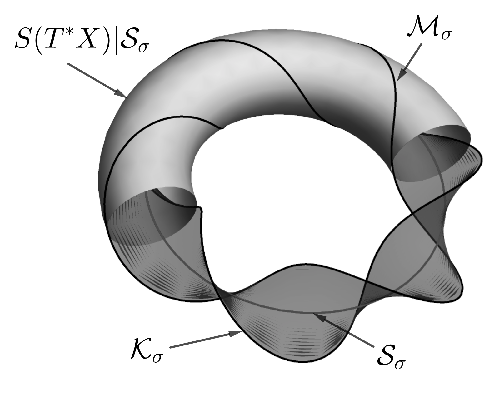
Figure 2.2. The multiplicity set ℳσ\mathcal{M}_{\sigma} as the intersection of the kernel bundle 𝒦σ\mathcal{K}_{\sigma} with S⁡(T∗​X|𝒮σ)S(T^{*}X|\mathcal{S}_{\sigma}).

The sets 𝒦σ\mathcal{K}_{\sigma} and ℳσ\mathcal{M}_{\sigma} are related as follows (see Figure 2.2)

ℳσ=S⁡(T∗​X)∩𝒦σ​ and ​𝒦σ=ℝ⋅ℳσ,\mathcal{M}_{\sigma}=S(T^{*}X)\cap\mathcal{K}_{\sigma}\hbox{\,\,and\,\,}\mathcal{K}_{\sigma}=\mathbb{R}\cdot\mathcal{M}_{\sigma},

where the action of λ∈ℝ\lambda\in\mathbb{R} on an element ξ∈ℳσ\xi\in\mathcal{M}_{\sigma} is that of scalar multiplication.

Remark 7.

The sets 𝒮σ,𝒦σ\mathcal{S}_{\sigma},\mathcal{K}_{\sigma} and ℳσ\mathcal{M}_{\sigma} only depend on the traceless part of σ\sigma. Hence, when studying these spaces we can assume that σ\sigma is a traceless symbol.

Theorem 8.

For a symbol σ\sigma in general position with 𝒮σ≠∅\mathcal{S}_{\sigma}\not=\emptyset we have that

  1. (1)

    The the singular set 𝒮σ\mathcal{S}_{\sigma} is a smooth 1-dimensional sub-manifold of XX.

  2. (2)

    The kernel bundle 𝒦σ\mathcal{K}_{\sigma} is a smooth rank one real vector bundle over 𝒮σ\mathcal{S}_{\sigma}.

  3. (3)

    The symbol σ0:S⁡(T∗​X)→S02​F\sigma_{0}:S(T^{*}X)\rightarrow\hbox{S}_{0}^{2}F is transversal to the zero section of S02​F\hbox{S}_{0}^{2}F.

Proof.

see section 5 ∎

Remark 9.

The importance of point 3 in the above Theorem is that for symbols σ\sigma in general position, the multiplicity set ℳσ\mathcal{M}_{\sigma} can be characterized as the set where the eigenvalue functions λσ,1|S⁡(T∗​X)\lambda_{\sigma,1}|S(T^{*}X) and λσ,2|S⁡(T∗​X)\lambda_{\sigma,2}|S(T^{*}X) are non-smooth (see Proposition 3).

We will now show that we can write

𝒦σ=Lσ|𝒮σ,\mathcal{K}_{\sigma}=L_{\sigma}|\mathcal{S}_{\sigma},

where LσL_{\sigma} is line sub-bundle of T∗​X|(X−Cσ)T^{*}X|(X-C_{\sigma}) and CσC_{\sigma} consists of a finite number of points. Recall that we have a metric gg in S02​F\hbox{S}_{0}^{2}F given by g⁡(A,B)=tr​(A∘B)/2.g(A,B)=\hbox{tr}(A\circ B)/2. Consider a traceless symbol σ\sigma and let σ∗:S02​F→T∗​X\sigma^{*}:\hbox{S}_{0}^{2}F\rightarrow T^{*}X be its adjoint. We define the section Gσ:X→S2​(T∗​X)G_{\sigma}:X\rightarrow\hbox{S}^{2}(T^{*}X) by Gσ=sσ∗∘σ,G_{\sigma}=s_{\sigma^{*}\circ\sigma}, so that

<Gσ​(x)​ξ,η>=g⁡(σ⁡(ξ),σ⁡(η)).<G_{\sigma}(x)\xi,\eta>=g(\sigma(\xi),\sigma(\eta)).

The eigenvalues of GσG_{\sigma} define functions κσ,1,κσ,2:X→ℝ\kappa_{\sigma,1},\kappa_{\sigma,2}:X\rightarrow\mathbb{R} with corresponding orthogonal eigen-line subfields Lσ,1L_{\sigma,1} and Lσ,2L_{\sigma,2} of T∗​X|(X−Cσ)T^{*}X|(X-C_{\sigma}), where

Cσ={x∈X|κσ,1​(x)=κσ,1​(x)}.C_{\sigma}=\{x\in X|\kappa_{\sigma,1}(x)=\kappa_{\sigma,1}(x)\}.

For symbols in general position CσC_{\sigma} is a finite set. The functions κσ,1\kappa_{\sigma,1} and κσ2\kappa_{\sigma_{2}} are non-negative and we can assume that κσ,1≤κσ,2\kappa_{\sigma,1}\leq\kappa_{\sigma,2}. We can then write

(2.3) 0≤κσ,1≤κσ,2.0\leq\kappa_{\sigma,1}\leq\kappa_{\sigma,2}.

By constructions we have

‖σ⁡(ξ)‖2=<Gσ​(x)​ξ,ξ>||\sigma(\xi)||^{2}=<G_{\sigma}(x)\xi,\xi>

so that for x∈X−Cσx\in X-C_{\sigma} and ξ∈S⁡(Tx∗​X)\xi\in S(T^{*}_{x}X) we have that

(2.4) ‖σ⁡(ξ)‖2=κσ,1​(x)​cos2⁡(θ⁡(x))+κσ,2​(x)​sin2⁡(θ⁡(x)),||\sigma(\xi)||^{2}=\kappa_{\sigma,1}(x)\cos^{2}(\theta(x))+\kappa_{\sigma,2}(x)\sin^{2}(\theta(x)),

where θ⁡(x)\theta(x) is the angle that ξ\xi makes with Lσ,1​(x)L_{\sigma,1}(x). The above formula still make sense for x∈Cσx\in C_{\sigma} since in this case, independently of how we define θ⁡(x)\theta(x), we have that ‖σ⁡(ξ)‖2=κσ,1​(x)=κσ,2​(x)||\sigma(\xi)||^{2}=\kappa_{\sigma,1}(x)=\kappa_{\sigma,2}(x).

Proposition 10.

For a traceless symbol σ\sigma in general position we have that κσ,2>0\kappa_{\sigma,2}>0 and

𝒮σ\displaystyle\mathcal{S}_{\sigma} ={x∈X|κσ,1​(x)=0},\displaystyle=\{x\in X|\kappa_{\sigma,1}(x)=0\},
𝒦σ\displaystyle\mathcal{K}_{\sigma} =Lσ,1|𝒮σ.\displaystyle=L_{\sigma,1}|\mathcal{S}_{\sigma}.
Proof.

If x∈Xx\in X is such that κ2​(x)=0\kappa_{2}(x)=0 from 2.3 and 2.4 we get 𝒦σ​(x)=Tx∗​X\mathcal{K}_{\sigma}(x)=T^{*}_{x}X, which contradicts Theorem 8. We conclude that kσ,2​(x)>0k_{\sigma,2}(x)>0 for all x∈Xx\in X. Hence

𝒮σ\displaystyle\mathcal{S}_{\sigma} ={x∈X|κσ,1​(x)=0},\displaystyle=\{x\in X|\kappa_{\sigma,1}(x)=0\},
𝒦σ\displaystyle\mathcal{K}_{\sigma} =ℝ⋅{ξ∈S⁡(T∗​X)|x∈𝒮σ​ and ​θ​(x)∈{0,π}}=Lσ,1​(x).\displaystyle=\mathbb{R}\cdot\{\xi\in S(T^{*}X)|x\in\mathcal{S}_{\sigma}\hbox{\,\,and\,\,}\theta(x)\in\{0,\pi\}\}=L_{\sigma,1}(x).

∎

2.5. The degree of the multiplicity set

Refer to caption
(a) deg⁡(ℳσ|C)=0\deg(\mathcal{M}_{\sigma}|C)=0
Refer to caption
(b) deg⁡(ℳσ|C)=1\deg(\mathcal{M}_{\sigma}|C)=1
Refer to caption
(c) deg⁡(ℳσ|C)=−5\deg(\mathcal{M}_{\sigma}|C)=-5
Figure 2.3. The degree of ℳσ\mathcal{M}_{\sigma} over a connected component CC of 𝒮σ\mathcal{S}_{\sigma}. The curve CC has been oriented counter-clockwise.

Consider a symbol σ\sigma in general position with non-empty singular set. The connected components of 𝒮σ\mathcal{S}_{\sigma} are 11-dimensional sub-manifolds of XX; each of them homeomorphic to a circle. An orientation of 𝒮σ\mathcal{S}_{\sigma} induces and orientation in ℳσ\mathcal{M}_{\sigma} that makes the projection map ξx↦x\xi_{x}\mapsto x orientation preserving. The degree of ℳσ\mathcal{M}_{\sigma} over a connected component CC of 𝒮σ\mathcal{S}_{\sigma} is the number of times that 𝒦σ\mathcal{K}_{\sigma} “turns with respect to CC” as we move along CC (see Figure 2.3); and the degree of ℳσ\mathcal{M}_{\sigma} is the sum of these numbers over all the connected components of 𝒮σ\mathcal{S}_{\sigma}. The technical details of this definition are as follows.

Consider the map μσ:ℳσ→S1\mu_{\sigma}:\mathcal{M}_{\sigma}\rightarrow S^{1}, where S1={z∈ℂ||z|=1}S^{1}=\{z\in\mathbb{C}||z|=1\}, defined by

μσ​(ξx)=ξx♯uσ​(x),\mu_{\sigma}(\xi_{x})=\frac{\xi_{x}^{\sharp}}{u_{\sigma}(x)},

where uσ:𝒮σ→T​𝒮σu_{\sigma}:\mathcal{S}_{\sigma}\rightarrow T\mathcal{S}_{\sigma} is a unit tangent field compatible with the orientation of 𝒮σ\mathcal{S}_{\sigma}; the quotient ξx#/uσ​(x)\xi_{x}^{\#}/u_{\sigma}(x) being defined as the unique complex number exp⁡(i​ψ)∈S1\exp(i\psi)\in S^{1} such that ξx#=exp⁡(i​ψ)​uσ​(x)\xi_{x}^{\#}=\exp(i\psi)u_{\sigma}(x).

Definition 11.

For a give orientation of 𝒮σ\mathcal{S}_{\sigma}, the degree of ℳσ\mathcal{M}_{\sigma} is the integer

deg⁡(ℳσ)=12​π​i​∫ℳσμσ∗​(d​zz)\deg(\mathcal{M}_{\sigma})=\frac{1}{2\pi i}\int_{\mathcal{M}_{\sigma}}\mu_{\sigma}^{*}\left(\frac{dz}{z}\right)

If we define the degree of ℳσ\mathcal{M}_{\sigma} over a connected component CC of 𝒮σ\mathcal{S}_{\sigma} as

deg⁡(ℳσ|C)=12​π​i​∫ℳσ|Cμσ∗​(d​zz)\deg(\mathcal{M}_{\sigma}|C)=\frac{1}{2\pi i}\int_{\mathcal{M}_{\sigma}|C}\mu_{\sigma}^{*}\left(\frac{dz}{z}\right)

then

deg⁡(ℳσ)=∑i=1kdeg⁡(ℳσ|Cσ,i),\deg(\mathcal{M}_{\sigma})=\text{$\sum_{i=1}^{k}\deg(\mathcal{M}_{\sigma}|C_{\sigma,i})$,}

where {Cσ,i}i=1k\{C_{\sigma,i}\}_{i=1}^{k} are the connected components of 𝒮σ\mathcal{S}_{\sigma}.

Remark.

If d​θd\theta is the angular form

d​θ=−y​d​xx2+y2+x​d​yx2+y2d\theta=\frac{-ydx}{x^{2}+y^{2}}+\frac{xdy}{x^{2}+y^{2}}

we can also write

deg⁡(ℳσ)=12​π​∫ℳσμσ∗​(𝑑θ).\deg(\mathcal{M}_{\sigma})=\frac{1}{2\pi}\int_{\mathcal{M}_{\sigma}}\mu_{\sigma}^{*}(d\theta).

It is important to notice that the definitions of deg⁡(ℳσ)\deg(\mathcal{M}_{\sigma}) and deg⁡(ℳσ|C)\deg(\mathcal{M}_{\sigma}|C) depend on the choice of orientation of 𝒮σ\mathcal{S}_{\text{$\sigma$}}; we will later see how to assign an “natural orientation” to 𝒮σ\mathcal{S}_{\sigma} in some cases of interest. Also, observe that set ℳσ|C\mathcal{M}_{\sigma}|C is connected if deg⁡(ℳσ|C)\deg(\mathcal{M}_{\sigma}|C) is odd and it consists of two connected components if deg⁡(ℳσ|C)\deg(\mathcal{M}_{\sigma}|C) is even.

Problem 12.

Given m∈ℤm\in\mathbb{Z} does there exists a symbol σ\sigma such that deg⁡(ℳσ)=m\deg(\mathcal{M}_{\sigma})=m?

2.6. Physical interpretation of the degree of ℳσ\mathcal{M}_{\sigma}

Refer to caption
Figure 2.4. Rays orthogonal to CC

Recall that when trying to find high frequency solutions to the partial differential equation associated with σ\sigma, we arrived at the Hamilton-Jacobi equations

∂φ∂t(x,t)+λσ,i(dxφ(x,t))=0, for i=1,2.\frac{\partial\varphi}{\partial t}(x,t)+\lambda_{\sigma,i}(d_{x}\varphi(x,t))=0,\hbox{\,\,for\,\,}i=1,2.

If the phase function has the form φ⁡(x,t)=ψ⁡(x)−t\varphi(x,t)=\psi(x)-t, we obtain

(2.5) λσ,i​(d​ψ​(x))=1​ for ​i=1,2.\lambda_{\sigma,i}(d\psi(x))=1\hbox{\,\,for\,\,}i=1,2.

Solutions to these equations can be obtained by the method of characteristics. A characteristic curve is an integral line of the Hamiltonian vector field of λσ,i\lambda_{\sigma,i}, and the corresponding ray is its projection onto XX. For a 11-dimensional submanifold CC of XX consider the characteristic curves contained in {ξ∈T∗​X|λσ,i​(ξ)=1}\{\xi\in T^{*}X|\lambda_{\sigma,i}(\xi)=1\} and whose corresponding rays are orthogonal to CC (see Figure 2.4). Solutions to 2.5 having CC as level set can be constructed (at least near CC) by letting

ψ⁡(x)=time of arrival of ray from ​C​ to ​x.\psi(x)=\hbox{time\,of\,arrival\,of\,ray\,from\,\,}C\hbox{\,\,to\,\,}x.

Consider the case when CC is a connected component of 𝒮σ\mathcal{S}_{\sigma}. Special optical phenomena occurs when the rays emerging from CC are tangent to lines in 𝒦σ\mathcal{K}_{\sigma}. The signed count of the points at which this happens is deg⁡(ℳσ|C)\deg(\mathcal{M}_{\sigma}|C) (see Figure 2.5) . In particular, the number of such points is bounded below by |deg⁡(ℳσ|C)||\deg(\mathcal{M}_{\sigma}|C)|.

Refer to caption
Figure 2.5. The kernel bundle 𝒦σ\mathcal{K}_{\sigma} over a connected component of the singular set 𝒮σ\mathcal{S}_{\sigma}. The lines A,B,C,DA,B,C,D and EE represent directions at which singular optical phenomena occur.

3. Symbols on the tangent bundle

In this section we will study symbols for the case when F=T​XF=TX. Under this assumption we will be able to give a formula to compute the degree of the multiplicity set ℳσ\mathcal{M}_{\sigma} in terms of the Euler characteristics of XX and a sub-manifold with boundary 𝒩σ⊂X\mathcal{N}_{\sigma}\subset X with ∂𝒩σ=𝒮σ\partial\mathcal{N}_{\sigma}=\mathcal{S}_{\sigma} (see Theorem 22).

3.1. Symbols as sections of complex line bundles

Since FF is an S​O​(2)=U⁡(1)SO(2)=U(1) vector bundle, we can also see it as complex line bundle. We will let F0F^{0} stand for the trivial complex line bundle X×ℂX\times\mathbb{C} and for n>0n>0 define

Fn\displaystyle F^{n} =F⊗ℂ⋯⊗ℂF,\displaystyle=F\otimes_{\mathbb{C}}\cdots\otimes_{\mathbb{C}}F,
F−n\displaystyle F^{-n} =F¯⊗ℂ⋯⊗ℂF¯,\displaystyle=\bar{F}\otimes_{\mathbb{C}}\cdots\otimes_{\mathbb{C}}\bar{F},

where F¯\bar{F} is the conjugate bundle of FF. If v∈Fxnv\in F_{x}^{n} and w∈Fxmw\in F_{x}^{m} then v⊗ℂw∈Fxm+nv\otimes_{\mathbb{C}}w\in F_{x}^{m+n}, and for simplicity we will write

v​w=v⊗ℂw.vw=v\otimes_{\mathbb{C}}w.

Since FF is a one dimensional complex line bundle we have that v​w=w​vvw=wv. Furthermore, the induced norms in FnF^{n} and FmF^{m} are such that |v​w|=|v|​|w||vw|=|v||w|. Every non-zero element v∈Fxnv\in F_{x}^{n} has an inverse element in v−1∈Fx−nv^{-1}\in F_{x}^{-n}, which is the unique vector satisfying v​v−1=1∈Fx0vv^{-1}=1\in F_{x}^{0}. Hence, for v∈Fxmv\in F_{x}^{m} and w∈Fxnw\in F_{x}^{n} we can define v/w=v​w−1∈Fxn−mv/w=vw^{-1}\in F_{x}^{n-m}.

The following result will allow us to identify traceless symbols σ\sigma in T​XTX with two of sections v:X→T​Xv:X\rightarrow TX and w:X→(T​X)3w:X\rightarrow(TX)^{3}. Recall that S2​F\hbox{S}^{2}F has a metric defined by

g⁡(A,B)=12​tr​(A∘B)​ for ​A,B∈S2​Fx.g(A,B)=\frac{1}{2}\hbox{tr}(A\circ B)\hbox{\,\,for\,\,}A,B\in\hbox{S}^{2}F_{x}.
Theorem 13.

Let FF be an SO​(2)\hbox{SO}(2) vector bundle of rank 22 over XX. There exists an isomorphism of real vector bundles Φ:F⊕F3→Hom​(F∗,S02​F)\Phi:F\oplus F^{3}\rightarrow\hbox{Hom}(F^{*},\hbox{S}_{0}^{2}F) such that if for v∈Fxv\in F_{x} and w∈Fx3w\in F_{x}^{3} we let σ=Φ⁡(v⊕w)\sigma=\Phi(v\oplus w), then the endomorphism Gσ:Fx∗→Fx∗G_{\sigma}:F_{x}^{*}\rightarrow F_{x}^{*} defined by

<Gσ​ξ,η>=g⁡(σ⁡(ξ),σ⁡(η)).<G_{\sigma}\xi,\eta>=g(\sigma(\xi),\sigma(\eta)).

has eigenvalues

κ1\displaystyle\kappa_{1} =12​(|v|−|w|)2,\displaystyle=\frac{1}{2}\left(|v|-|w|\right)^{2},
κ2\kappa_{2} =12​(|v|+|w|)2.\displaystyle=\frac{1}{2}\left(|v|+|w|\right)^{2}.

Furthermore, for v≠0v\not=0 and w≠0w\not=0 the eigen-spaces L1L_{1} and L2L_{2} corresponding to κ1\kappa_{1} and κ2\kappa_{2} are

L1\displaystyle L_{1} =ℝ⋅{z♭∈Fx∗|z2=w/v},\displaystyle=\mathbb{R}\cdot\{z^{\flat}\in F_{x}^{*}|z^{2}=w/v\},
L2\displaystyle L_{2} =ℝ⋅{z♭∈Fx∗|z2=−w/v}.\displaystyle=\mathbb{R}\cdot\{z^{\flat}\in F_{x}^{*}|z^{2}=-w/v\}.
Proof.

See section 6 ∎

Corollary 14.

For any traceless symbol σ:T∗​X→S02​(T​X)\sigma:T^{*}X\rightarrow\hbox{S}_{0}^{2}(TX) we can find unique sections v:X→T​Xv:X\rightarrow TX and w:X→(T​X)3w:X\rightarrow(TX)^{3} such that

σ=σs​ where ​s​(x)=Φ⁡(v⁡(x)⊕w⁡(x)).\sigma=\sigma_{s}\hbox{\,\,\,where\,\,\,}s(x)=\Phi(v(x)\oplus w(x)).

In this case we have that

𝒮σ={x∈X||w⁡(x)/v⁡(x)|=1},\mathcal{S}_{\sigma}=\{x\in X||w(x)/v(x)|=1\},

and

ℳσ=⋃x∈𝒮σ{z♭∈Tx∗​X|z∈Tx​X​ and ​z2=w⁡(x)v⁡(x)}.\mathcal{M}_{\sigma}=\bigcup_{x\in\mathcal{S}_{\sigma}}\left\{z^{\flat}\in T^{*}_{x}X|z\in T_{x}X\hbox{\,\,and\,\,}z^{2}=\frac{w(x)}{v(x)}\right\}.
Proof.

The result follows directly from Theorem 13 and Proposition 10 by letting vv and ww be given by

v⁡(x)⊕w⁡(x)=Φ−1​(sσ​(x)),v(x)\oplus w(x)=\Phi^{-1}(s_{\sigma}(x)),

∎

Definition 15.

For sections v:X→T​Xv:X\rightarrow TX and w:X→(T​X)3w:X\rightarrow(TX)^{3} we will refer to the traceless symbol σv,w:T∗​X→S02​(T​X)\sigma_{v,w}:T^{*}X\rightarrow\hbox{S}_{0}^{2}(TX) given by

σv,w=σs​ for ​s​(x)=Φ⁡(v⁡(x)⊕w⁡(x)),\sigma_{v,w}=\sigma_{s}\hbox{\,\,\,for\,\,\,}s(x)=\Phi(v(x)\oplus w(x)),

as the symbol associated vv and ww.

Remark 16.

For the symbol σ=σv,w\sigma=\sigma_{v,w} formula 2.4 becomes

‖σ⁡(ξx)‖2=12​(|v⁡(x)|2+|w⁡(x)|2−2​|v⁡(x)|​|w⁡(x)|​cos⁡(2​θ​(x))).||\sigma(\xi_{x})||^{2}=\frac{1}{2}\left(|v(x)|^{2}+|w(x)|^{2}-2|v(x)||w(x)|\cos(2\theta(x))\right).

3.2. A formula for the degree of ℳσ\mathcal{M}_{\sigma}

If CC is a 1-dimensional compact oriented sub-manifold of XX and v1,v2:C→Fn|Cv_{1},v_{2}:C\rightarrow F^{n}|C are non-vanishing sections, we define the degree of v2v_{2} with respect to v1v_{1} as the integer

degv1⁡(v2)=12​π​i​∫Cμ∗​(d​zz),\deg_{v_{1}}(v_{2})=\frac{1}{2\pi i}\int_{C}\mu^{*}\left(\frac{dz}{z}\right),

where μ:C→ℂ−{0}\mu:C\rightarrow\mathbb{C}-\{0\} is given by

μ⁡(x)=v2​(x)v1​(x).\mu(x)=\frac{v_{2}(x)}{v_{1}(x)}.

If {Ck}1≤i≤n\{C_{k}\}_{1\leq i\leq n} are the connected components of CC and {γk:[ak,bk]→Ck}1≤k≤n\{\gamma_{k}:[a_{k},b_{k}]\rightarrow C_{k}\}_{1\leq k\leq n} are orientation preserving parametrization maps, then

degv1⁡(v2)=12​π​i​∑k=1n∫akbk(μ˙k​(t)μk​(t))​𝑑t​ where μk​(t)=μ⁡(γk​(t)).\deg_{v_{1}}(v_{2})=\frac{1}{2\pi i}\sum_{k=1}^{n}\int_{a_{k}}^{b_{k}}\left(\frac{\dot{\mu}_{k}(t)}{\mu_{k}(t)}\right)dt\hbox{\,\,where\,\,}\text{$\mu_{k}(t)=\mu(\gamma_{k}(t)).$}

It is easy to verify that if v1,v2v_{1},v_{2} are non-vanishing sections of FnF^{n} and w1,w2w_{1},w_{2} are non-vanishing sections of FmF^{m}, then

degv1​w1⁡(v2​w2)=degv1⁡(v2)+degw1⁡(w2).\deg_{v_{1}w_{1}}(v_{2}w_{2})=\deg_{v_{1}}(v_{2})+\deg_{w_{1}}(w_{2}).
Definition 17.

For a non-vanishing section v:C→(T​X)n|Cv:C\rightarrow(TX)^{n}|C the degree of vv with respect to CC is the integer

degC⁡(v)=degun⁡(v),\deg_{C}(v)=\deg_{u^{n}}(v),

where u:C→T​Cu:C\rightarrow TC is a unit tangent field compatible with the orientation of CC.

Proposition 18.

Consider sections v:X→T​Xv:X\rightarrow TX and w:X→(T​X)3w:X\rightarrow(TX)^{3} with no common zeros. If σ=σv,w\sigma=\sigma_{v,w} and CC is a connected component of 𝒮σ\mathcal{S}_{\sigma} then

deg⁡(ℳσ|C)=degC⁡(w)−degC⁡(v),\deg(\mathcal{M}_{\sigma}|C)=\deg_{C}(w)-\deg_{C}(v),

and hence

deg⁡(ℳσ)=deg𝒮σ⁡(w)−deg𝒮σ⁡(v).\deg(\mathcal{M}_{\sigma})=\deg_{\mathcal{S}_{\sigma}}(w)-\deg_{\mathcal{S}_{\sigma}}(v).
Proof.

The set ℳσ\mathcal{M}_{\sigma} consists of the elements of the form z♭​(x)∈T∗​X|𝒮σz^{\flat}(x)\in T^{*}X|\mathcal{S}_{\sigma} such that z⁡(x)∈T​X|𝒮σz(x)\in TX|\mathcal{S}_{\sigma} satisfies

z⁡(x)=±(w⁡(x)v⁡(x))1/2.z(x)=\pm\left(\frac{w(x)}{v(x)}\right)^{1/2}.

This formula can be re-written as

z⁡(x)u⁡(x)=±(h⁡(x))1/2\frac{z(x)}{u(x)}=\pm(h(x))^{1/2}

for h:𝒮σ→ℂ−{0}h:\mathcal{S}_{\sigma}\rightarrow\mathbb{C}-\{0\} given by

h⁡(x)=(v⁡(x)u⁡(x))−1​(w⁡(x)u3​(x)),h(x)=\left(\frac{v(x)}{u(x)}\right)^{-1}\left(\frac{w(x)}{u^{3}(x)}\right),

where u⁡(x)∈Tx​𝒮σu(x)\in T_{x}\mathcal{S}_{\sigma} is unitary and compatible with the orientation of 𝒮σ\mathcal{S}_{\sigma}. If γ:[a,b]→C\gamma:[a,b]\rightarrow C is an orientation preserving arc-length parametrization of CC then u​(t)=γ˙​(t)u(t)=\dot{\gamma}(t). If we write z⁡(t)=z⁡(γ⁡(t)),v⁡(t)=v⁡(γ⁡(t)),w⁡(t)=w⁡(γ⁡(t)),h⁡(t)=h⁡(γ⁡(t))z(t)=z(\gamma(t)),v(t)=v(\gamma(t)),w(t)=w(\gamma(t)),h(t)=h(\gamma(t)), and let ψ,θ:[a,b]→ℝ\psi,\theta:[a,b]\rightarrow\mathbb{R} be continuous functions such that

w⁡(t)u3​(t)=|w⁡(t)|exp⁡(i​ψ​(t))​ and ​v⁡(t)u⁡(t)=|v⁡(t)|​exp⁡(i​θ​(t)),\frac{w(t)}{u^{3}(t)}=|w(t)|\exp(i\psi(t))\hbox{\,\,and\,\,\,\,}\frac{v(t)}{u(t)}=|v(t)|\exp(i\theta(t)),

then

deg⁡(w|C)\displaystyle\deg(w|C) =ψ⁡(b)−ψ⁡(a)2​π,\displaystyle=\frac{\psi(b)-\psi(a)}{2\pi},
deg⁡(v|C)\displaystyle\deg(v|C) =θ⁡(b)−θ⁡(a)2​π.\displaystyle=\frac{\theta(b)-\theta(a)}{2\pi}.

Since γ⁡(t)∈𝒮σ\gamma(t)\in\mathcal{S}_{\sigma}, we have that |w⁡(t)|=|v⁡(t)||w(t)|=|v(t)| and hence

h⁡(t)=exp⁡(i​φ​(t))​ where ​φ​(t)=ψ⁡(t)−θ⁡(t).h(t)=\exp\left(i\varphi(t)\right)\hbox{\,\,where\,\,}\varphi(t)=\psi(t)-\theta(t).

From the above we conclude that

z⁡(t)u⁡(t)=exp⁡(i​φ​(t)/2)​ or ​z⁡(t)u⁡(t)=exp⁡(i⁡(φ⁡(t)+π)/2),\frac{z(t)}{u(t)}=\exp(i\varphi(t)/2)\hbox{\,\,or\,\,\,}\frac{z(t)}{u(t)}=\exp(i(\varphi(t)+\pi)/2),

and hence

deg⁡(ℳσ|C)\displaystyle\deg(\mathcal{M}_{\sigma}|C) =12​π​((φ⁡(b)−φ⁡(a)2)+((φ⁡(b)+π)−(φ⁡(a)+π)2))\displaystyle=\frac{1}{2\pi}\left(\left(\frac{\varphi(b)-\varphi(a)}{2}\right)+\left(\frac{(\varphi(b)+\pi)-(\varphi(a)+\pi)}{2}\right)\right)
=φ⁡(b)−φ⁡(a)2​π\displaystyle=\frac{\varphi(b)-\varphi(a)}{2\pi}
=ψ⁡(b)−ψ⁡(a)2​π−θ⁡(b)−θ⁡(a)2​π\displaystyle=\frac{\psi(b)-\psi(a)}{2\pi}-\frac{\theta(b)-\theta(a)}{2\pi}
=deg⁡(w|C)−deg⁡(v|C).\displaystyle=\deg(w|C)-\deg(v|C).

The second part of the proposition is a direct consequence of the first part. ∎

We will denote the set of zeros of a section v:X→(T​X)nv:X\rightarrow(TX)^{n} as ZvZ_{v}. If x∈Xx\in X is an isolated zero of vv, the degree of vv at xx can be computed as

degx⁡(v)=degw|∂D⁡(v),\deg_{x}(v)=\deg_{w|\partial D}(v),

where DD is a “small disk” with Zv​∩D={x}Z_{v}\text{$\cap D=\{x\}$} and w:D→(T​X)n|Dw:D\rightarrow(TX)^{n}|D is a non-vanishing vector field.

Proposition 19.

Let Y⊂XY\subset X be a 2-dimensional manifold with boundary ∂Y\partial Y, and consider sections u,v:Y→(T​X)n|Yu,v:Y\rightarrow(TX)^{n}|Y whose zero sets ZuZ_{u} and ZvZ_{v} are such that (Zu∪Zv)∩Y(Z_{u}\cup Z_{v})\cap Y is finite and Zu∩∂Y=Zv∩∂Y=∅Z_{u}\cap\partial Y=Z_{v}\cap\partial Y=\emptyset. We have that

degu|∂Y⁡(v)=∑x∈Zv∩Ydegx⁡(v)−∑x∈Zu∩Ydegx⁡(u).\deg_{u|\partial Y}(v)=\sum_{x\in Z_{v}\cap Y}\deg_{x}(v)-\sum_{x\in Z_{u}\cap Y}\deg_{x}(u).
Proof.

Let Y0Y_{0} be the set obtained from YY by removing a family of small open disks {Dx}x∈(Zu∪Zv)∩Y\{D_{x}\}_{x\in(Z_{u}\cup Z_{v})\cap Y}, where each DxD_{x} contains xx and each DxD_{x} is contained in the interior of YY. Consider the map μ:Y0→ℂ−{0}\mu:Y_{0}\rightarrow\mathbb{C}-\{0\} defined by

μ⁡(x)=v⁡(x)u⁡(x).\mu(x)=\frac{v(x)}{u(x)}.

Using Stokes Theorem and the fact that the form d​z/zdz/z is closed in ℂ−{0}\mathbb{C}-\{0\}, we obtain

∫∂Y0μ∗​(d​zz)=0.\int_{\partial Y_{0}}\mu^{*}\left(\frac{dz}{z}\right)=0.

From this and the formula

∂Y0=∂Y−∑x∈(Zu∪Zv)∩Y∂Dx,\partial Y_{0}=\partial Y-\sum_{x\in(Z_{u}\cup Z_{v})\cap Y}\partial D_{x},

we obtain

degu|∂Y⁡(v)=12​π​i​∑x∈(Zu∪Zv)∩Y∫∂Dxμ∗​(d​zz).\deg_{u|\partial Y}(v)=\frac{1}{2\pi i}\sum_{x\in(Z_{u}\cup Z_{v})\cap Y}\int_{\partial D_{x}}\mu^{*}\left(\frac{dz}{z}\right).

Since we can write

vu=v/wxnu/wxn,\frac{v}{u}=\frac{v/w_{x}^{n}}{u/w_{x}^{n}},

for wx:Dx→T​X|Dxw_{x}:D_{x}\rightarrow TX|D_{x} a non-vanishing vector field, we have

12​π​i​∫∂Dxμ∗​(d​zz)=degx⁡(v)−degx⁡(u).\frac{1}{2\pi i}\int_{\partial D_{x}}\mu^{*}\left(\frac{dz}{z}\right)=\deg_{x}(v)-\deg_{x}(u).

We conclude that

degu|∂Y=12​π​i​(∑x∈(Zu∪Zv)∩Ydegx⁡(v)−∑x∈(Zu∪Zv)∩Ydegx⁡(u)).\deg_{u|\partial Y}=\frac{1}{2\pi i}\left(\sum_{x\in(Z_{u}\cup Z_{v})\cap Y}\deg_{x}(v)-\sum_{x\in(Z_{u}\cup Z_{v})\cap Y}\deg_{x}(u)\right).

The result of the Proposition then follows from the formulas

∑x∈(Zu∪Zv)∩Ydegx⁡(v)\displaystyle\sum_{x\in(Z_{u}\cup Z_{v})\cap Y}\deg_{x}(v) =∑x∈Zv∩Ydegx⁡(v)+∑x∈(Zu−Zv)∩Ydegx⁡(v),\displaystyle=\sum_{x\in Z_{v}\cap Y}\deg_{x}(v)+\sum_{x\in(Z_{u}-Z_{v})\cap Y}\deg_{x}(v),
∑x∈(Zu∪Zv)∩Ydegx⁡(u)\displaystyle\sum_{x\in(Z_{u}\cup Z_{v})\cap Y}\deg_{x}(u) =∑x∈Zu∩Ydegx⁡(u)+∑x∈(Zv−Zu)∩Ydegx⁡(u),\displaystyle=\sum_{x\in Z_{u}\cap Y}\deg_{x}(u)+\sum_{x\in(Z_{v}-Z_{u})\cap Y}\deg_{x}(u),

and observing that degx⁡(v)=0\deg_{x}(v)=0 for x∈Zu−Zvx\in Z_{u}-Z_{v} and degx⁡(u)=0\deg_{x}(u)=0 for x∈Zv−Zux\in Z_{v}-Z_{u}. ∎

Remark 20.

When using Stoke’s Theorem in the proof of the above Proposition we implicitly assumed that ∂Y\partial Y is oriented by the field u=i​nu=in, where n:∂Y→T​X|∂Yn:\partial Y\rightarrow TX|\partial Y is the unit normal field to ∂Y\partial Y that points to the outside of YY.

Corollary 21.

Let f:X→ℝf:X\rightarrow\mathbb{R} be a smooth function having 00 as a regular value, and let

Y={x∈X|f⁡(x)≤0}.Y=\{x\in X|f(x)\leq 0\}.

If v:X→(T​X)nv:X\rightarrow(TX)^{n} does not vanish in ∂Y\partial Y and has a finite number of zeros in Y,Y, then

deg∂Y⁡(v)=∑x∈Zv∩Ydegx⁡(v)−n​χ​(Y).\deg_{\partial Y}(v)=\sum_{x\in Z_{v}\cap Y}\deg_{x}(v)-n\chi(Y).
Proof.

Let gg be a small perturbation of ff that makes gg a Morse function. The gradient field ∇f\nabla f points to the outside of YY. By choosing gg close enough to ff we can ensure that ∇g\nabla g will also point to the outside of YY and

deg(∇f)n|∂Y⁡(v)=deg(∇g)n|∂Y⁡(v).\deg_{(\nabla f)^{n}|\partial Y}(v)=\deg_{(\nabla g)^{n}|\partial Y}(v).

Using this formula and the fact that i∇f/|∇f|i\nabla f/|\nabla f| is the unit tangent field to ∂Y\partial Y compatible with its orientation, we obtain

deg∂Y⁡(v)\displaystyle\deg_{\partial Y}(v) =deg(i∇f/|∇f|)n|∂Y(v)\displaystyle=\deg_{(i\nabla f/|\nabla f|)^{n}|\partial Y}(v)
=deg(∇f)n|∂Y⁡(v)\displaystyle=\deg_{(\nabla f)^{n}|\partial Y}(v)
=deg(∇g)n|∂Y⁡(v).\displaystyle=\deg_{(\nabla g)^{n}|\partial Y}(v).

Since gg is a Morse function the set of critical points CgC_{g} of gg must be finite. Furthermore, since gg is close to ff and 00 is a regular value of ff, we have that none of the zeros of ∇g\nabla g can be in ∂Y.\partial Y. Hence, we can apply Proposition 19 to obtain

deg∂Y⁡(v)\displaystyle\deg_{\partial Y}(v) =∑x∈Y∩Zvdegx⁡(v)−∑x∈Y∩Cgdegx⁡((∇g)n)\displaystyle=\sum_{x\in Y\cap Z_{v}}\deg_{x}(v)-\sum_{x\in Y\cap C_{g}}\deg_{x}((\nabla g)^{n})
=∑x∈Y∩Zvdegx⁡(v)−n​∑x∈Y∩Cgdegx⁡(∇g)\displaystyle=\sum_{x\in Y\cap Z_{v}}\deg_{x}(v)-n\sum_{x\in Y\cap C_{g}}\deg_{x}(\nabla g)

The result now follows from the fact that ∇g\nabla g points to the outside of YY, so that (see [9])

∑x∈Y∩Cgdegx⁡(∇g)=χ⁡(Y).\sum_{x\in Y\cap C_{g}}\deg_{x}(\nabla g)=\chi(Y).

∎

Theorem 22.

Let σ=σv,w\sigma=\sigma_{v,w} be a traceless symbol in general position. The set

𝒩σ={x∈X||w⁡(x)/v⁡(x)|≤1}\mathcal{N}_{\sigma}=\{x\in X||w(x)/v(x)|\leq 1\}

is a smooth manifold with boundary and

deg⁡(ℳσ)=3​χ​(X)−2​χ​(𝒩σ).\deg(\mathcal{M}_{\sigma})=3\chi(X)-2\chi(\mathcal{N}_{\sigma}).
Proof.

For symbols in general position the function

f⁡(x)=|w⁡(x)v⁡(x)|−1f(x)=\left|\frac{w(x)}{v(x)}\right|-1

has 00 as a regular value, which implies that 𝒩σ\mathcal{N}_{\sigma} is a smooth manifold with boundary. Using Proposition 18 we obtain

deg⁡(ℳσ)=deg𝒮σ⁡(w)−deg𝒮σ⁡(v).\deg(\mathcal{M}_{\sigma})=\deg_{\mathcal{S}_{\sigma}}(w)-\deg_{\mathcal{S}_{\sigma}}(v).

Since 𝒮σ=∂𝒩σ\mathcal{S}_{\sigma}=\partial\mathcal{N}_{\sigma}, by Corollary 21 we have that

deg𝒮σ⁡(w)\displaystyle\deg_{\mathcal{S}_{\sigma}}(w) =∑x∈Zw∩𝒩σdegx⁡(w)−3​χ​(𝒩σ),\displaystyle=\sum_{x\in Z_{w}\cap\mathcal{N}_{\sigma}}\deg_{x}(w)-3\chi(\mathcal{N}_{\sigma}),
deg𝒮σ⁡(v)\displaystyle\deg_{\mathcal{S}_{\sigma}}(v) =∑x∈Zv∩𝒩σdegx⁡(v)−χ⁡(𝒩σ).\displaystyle=\sum_{x\in Z_{v}\cap\mathcal{N}_{\sigma}}\deg_{x}(v)-\chi(\mathcal{N}_{\sigma}).

For symbols in general position Zv∩Zw=∅Z_{v}\cap Z_{w}=\emptyset and hence Zv∩𝒩σ=∅Z_{v}\cap\mathcal{N}_{\sigma}=\emptyset, since v⁡(x)=0v(x)=0 for x∈𝒩σx\in\mathcal{N}_{\sigma} would imply that w⁡(x)=0w(x)=0. We conclude that

deg⁡(ℳσ)=∑x∈Zw∩𝒩σdegx⁡(w)−2​χ​(𝒩σ)\deg(\mathcal{M}_{\sigma})=\sum_{x\in Z_{w}\cap\mathcal{N}_{\sigma}}\deg_{x}(w)-2\chi(\mathcal{N}_{\sigma})

Using the fact that Zw⊂𝒩σZ_{w}\subset\mathcal{N}_{\sigma}, we obtain

∑x∈Zw∩𝒩σdegx⁡(w)=∑x∈Zwdegx⁡(w)=∫Xe⁡((T​X)3)=3​χ​(X).\sum_{x\in Z_{w}\cap\mathcal{N}_{\sigma}}\deg_{x}(w)=\sum_{x\in Z_{w}}\deg_{x}(w)=\int_{X}e\left((TX)^{3}\right)=3\chi(X).

Hence

deg⁡(ℳσ)=3​χ​(X)−2​χ​(𝒩σ).\deg(\mathcal{M}_{\sigma})=3\chi(X)-2\chi(\mathcal{N}_{\sigma}).

∎

Remark 23.

From the proof of the above Theorem we can see that if DD is a connected component of 𝒩σ\mathcal{N}_{\sigma}, then

(3.1) deg⁡(ℳσ|∂D)=(∑x∈Zv∩Ddegx⁡(w))−2​χ​(D).\deg(\mathcal{M}_{\sigma}|\partial D)=\left(\sum_{x\in Z_{v}\cap D}\deg_{x}(w)\right)-2\chi(D).

4. Examples

4.1. Holomorphic symbols on the complex plane

Refer to caption
(a) r0=1r_{0}=1
Refer to caption
(b) r0=1/3r_{0}=1/3
Figure 4.1. Equipotential curves for five negative charges at the 55-th roots of unity, and one positive charge at 00. The shaded regions represent the set 𝒩σ\mathcal{N}_{\sigma} for the given value of r0r_{0}.

Although we have assumed throughout the paper that the surface XX is compact, it will be instructive to study symbols on the plane ℝ2=ℂ\mathbb{R}^{2}=\mathbb{C}. We can write the traceless part of such symbols as σ=σv,w\sigma=\sigma_{v,w} for

v⁡(z)=a⁡(z)​∂∂x​ and ​w​(z)=b⁡(z)​(∂∂x)3,v(z)=a(z)\frac{\partial}{\partial x}\hbox{\,\,and\,\,}w(z)=b(z)\left(\frac{\partial}{\partial x}\right)^{3},

where a,ba,b and complex valued functions on the complex plane. Since we are using the flat metric in ℂ=ℝ2\mathbb{C}=\mathbb{R}^{2} we have that

|v⁡(z)|=|a⁡(z)​| and |​w​(z)|=|b⁡(z)|,|v(z)|=|a(z)|\text{\hbox{\,\,and\,\,}}|w(z)|=|b(z)|,

and hence

𝒮σ={z∈ℂ||b⁡(z)/a⁡(z)|=1}.\mathcal{S}_{\sigma}=\{z\in\mathbb{C}||b(z)/a(z)|=1\}.

If aa and bb are complex polynomials

a⁡(z)=a0​Πi=1na​(z−ai)​ and ​b​(z)=b0​Πj=1nb​(z−bi)a(z)=a_{0}\Pi_{i=1}^{n_{a}}(z-a_{i})\hbox{\,\,and\,\,}b(z)=b_{0}\Pi_{j=1}^{n_{b}}(z-b_{i})

then 𝒮σ\mathcal{S}_{\sigma} consists of the points z∈ℂz\in\mathbb{C} that satisfy the equation

(4.1) ∑i=1nalog⁡(1|z−ai|)−∑j=1nblog⁡(1|z−bi|)=r0,\sum_{i=1}^{n_{a}}\log\left(\frac{1}{|z-a_{i}|}\right)-\sum_{j=1}^{n_{b}}\log\left(\frac{1}{|z-b_{i}|}\right)=r_{0},

where

r0=log⁡(|a0||b0|).r_{0}=\log\left(\frac{|a_{0}|}{|b_{0}|}\right).

The harmonic function z↦log⁡(1/|z−p|)z\mapsto\log(1/|z-p|) represents the potential of a positively charged particle at pp. We conclude that 𝒮σ\mathcal{S}_{\sigma} is an equipotential curve of a superposition of positively and negatively charged particles. The negative charges are inside of 𝒩σ\mathcal{N}_{\sigma} and the positive charges outside of it.

Example 24.

Let us assume there are no positive charges for a n≥1n\geq 1 let b⁡(z)=znb(z)=z^{n}. For r0=0r_{0}=0 the set 𝒩σ\mathcal{N}_{\sigma} is the unit disk, and hence χ⁡(𝒩σ)=1\chi(\mathcal{N}_{\sigma})=1. Since deg0⁡(b)=n\deg_{0}(b)=n, using Formula 3.1 we obtain

deg⁡(ℳσ)=n−2.\deg(\mathcal{M}_{\sigma})=n-2.
Example 25.

Consider the case where we have 55 negative charges located at 55-th roots of unity and one positive charge at 00. For r0=1r_{0}=1 the set 𝒩σ\mathcal{N}_{\sigma} is a topological annulus (see Figure 4.1a) so that χ⁡(𝒩σ)=0\chi(\mathcal{N}_{\sigma})=0, and hence

deg⁡(ℳσ)=5−2​χ​(𝒩σ)=5.\deg(\mathcal{M}_{\sigma})=5-2\chi(\mathcal{N}_{\sigma})=5.

For r0=1/3r_{0}=1/3 the set 𝒩σ\mathcal{N}_{\sigma} consists of 5 topological discs (see Figure 4.1b) so that χ⁡(𝒩σ)=5\chi(\mathcal{N}_{\sigma})=5, and hence

deg⁡(ℳσ)=5−2​χ​(𝒩σ)=−5.\deg(\mathcal{M}_{\sigma})=5-2\chi(\mathcal{N}_{\sigma})=-5.

4.2. Holomorphic symbols on the sphere
Refer to caption
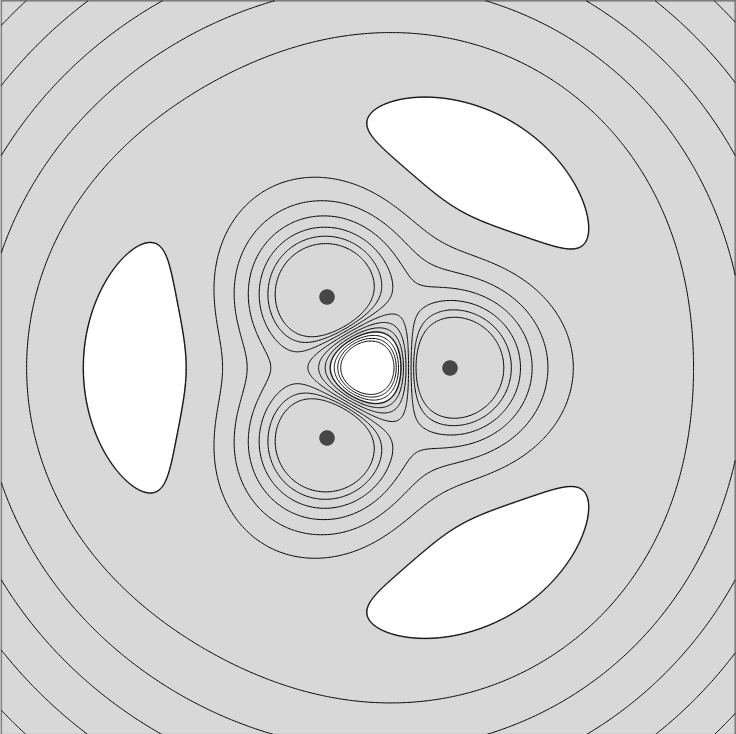
Figure 4.2. Equipotential lines of 3 negatively charges on the sphere. The shaded region represents the set 𝒩σ⊂S2\mathcal{N}_{\sigma}\subset S^{2}.

We consider the sphere as the Riemann sphere. The vector fields in T​S2TS^{2} and (T​S2)3(TS^{2})^{3} in zz-coordinates have the form

v⁡(z)=a⁡(z)​∂∂x​ and ​w​(z)=b⁡(z)​(∂∂x)3.v(z)=a(z)\frac{\partial}{\partial x}\hbox{\,\,and\,\,}w(z)=b(z)\left(\frac{\partial}{\partial x}\right)^{3}.

The metric in S2S^{2} is such that

|∂∂x|=21+|z|2​ for ​∂∂x∈Tz​S2,\left|\frac{\partial}{\partial x}\right|=\frac{2}{1+|z|^{2}}\hbox{\,\,\,for\,\,\,}\frac{\partial}{\partial x}\in T_{z}S^{2},

and hence

|v⁡(z)|=2​|a⁡(z)|1+|z|2​ and ​|w⁡(z)|=8​|b⁡(z)|(1+|z|2)3.|v(z)|=\frac{2|a(z)|}{1+|z|^{2}}\hbox{\,\,and\,\,}|w(z)|=\frac{8|b(z)|}{(1+|z|^{2})^{3}}.

We conclude that 𝒮σ\mathcal{S}_{\sigma} consists of the points zz satisfying

(4.2) (4(1+|z|2)2)​|b⁡(z)||a⁡(z)|=1.\left(\frac{4}{(1+|z|^{2})^{2}}\right)\frac{|b(z)|}{|a(z)|}=1.

If we denote the complex variables at 00 and ∞\infty by z=x+i​yz=x+iy and w=u+i​vw=u+iv, the change of variables formula is

w=1z,w=\frac{1}{z},

so that

∂∂x=−z−2​∂∂u.\frac{\partial}{\partial x}=-z^{-2}\frac{\partial}{\partial u}.

From this it follows that for any quadratic polynomial P⁡(z)=a0+a1​z+a2​z2P(z)=a_{0}+a_{1}z+a_{2}z^{2} the field

z↦P⁡(z)​∂∂x=(a0+a1​z+a2​z2)​∂∂xz\mapsto P(z)\frac{\partial}{\partial x}=(a_{0}+a_{1}z+a_{2}z^{2})\frac{\partial}{\partial x}

extends to a vector field over the whole sphere S2S^{2}. In fact, in ww coordinates the above field is written as

w↦−w2​P​(1/w)​∂∂u=−(a2+a1​w+a0​w2)​∂∂u.w\mapsto-w^{2}P(1/w)\frac{\partial}{\partial u}=-(a_{2}+a_{1}w+a_{0}w^{2})\frac{\partial}{\partial u}.

Suppose that aa is a polynomial of degree nan_{a} and bb a polynomial of degree nbn_{b}. From the above discussion we conclude that for 0≤na≤20\leq n_{a}\leq 2 and 0≤nb≤60\leq n_{b}\leq 6 the sections

z↦a⁡(z)​∂∂x​ and ​z↦b⁡(z)​(∂∂x)3z\mapsto a(z)\frac{\partial}{\partial x}\hbox{\,\,and\,\,}z\mapsto b(z)\left(\frac{\partial}{\partial x}\right)^{3}

correspond to a traceless symbols on T​S2TS^{2}. Equation 4.2 for the singularity can be written

(4.3) 2​log⁡(21+|z|2)+∑i=1nalog⁡(1|z−ai|)−∑i=1nblog⁡(1|z−bi|)=r02\log\left(\frac{2}{1+|z|^{2}}\right)+\sum_{i=1}^{n_{a}}\log\left(\frac{1}{|z-a_{i}|}\right)-\sum_{i=1}^{n_{b}}\log\left(\frac{1}{|z-b_{i}|}\right)=r_{0}

where r0=log⁡(|a0|/|b0|)r_{0}=\log(|a_{0}|/|b_{0}|). This formula is very similar to the one we have studied for symbols in the plane, but for the appearance of the first term which accounts for the fact that we are working on the sphere.

Example 26.

Let us assume that there are no positive charges and that b⁡(z)=znb(z)=z^{n}. Some simple calculations show that for for n=1n=1 the set 𝒩σ\mathcal{N}_{\sigma} consists of two topological disks on S2S^{2}, and for n=4n=4 the set 𝒩σ\mathcal{N}_{\sigma} consists of a single topological disk on S2S^{2}. Using Theorem 22 we obtain

deg⁡(ℳσ)={2 for ​n=1,4 for ​n=4.\deg(\mathcal{M}_{\sigma})=\begin{cases}2&\hbox{\,\,for\,\,}n=1,\\ 4&\hbox{\,\,for\,\,}n=4.\end{cases}
Example 27.

Let us assume that there are no positive charges and that we have 33 negative charges located at 1/3,exp⁡(2​π/3)/3,exp⁡(4​π/3)/31/3,\exp(2\pi/3)/3,\exp(4\pi/3)/3 . The set 𝒩σ⊂S2\mathcal{N}_{\sigma}\subset S^{2} has 4 holes (see Figure 4.2) so that χ⁡(𝒩σ)=−3\chi(\mathcal{N}_{\sigma})=-3, an hence

deg⁡(ℳσ)=12.\deg(\mathcal{M}_{\sigma})=12.

5. Proof of theorem 8

We will prove a slightly more general result. Let E1E_{1} and E2E_{2} be SO​(2)\hbox{SO}(2) vector bundles of rank 22 over a surface XX; for our particular case E1=T∗​XE_{1}=T^{*}X and E2=S02​FE_{2}=\hbox{S}_{0}^{2}F. The bundle of homomorphisms Hom​(E1,E2)\hbox{Hom}(E_{1},E_{2}) stratifies as

Hom​(E1,E2)=⋃i=02[Hom​(E1,E2)]i\hbox{Hom}(E_{1},E_{2})=\bigcup_{i=0}^{2}[\hbox{Hom}(E_{1},E_{2})]_{i}

where

[Hom(E1,E2)]i={A∈Hom(E1,E2)|dim(ker(A)=i},[\hbox{Hom}(E_{1},E_{2})]_{i}=\{A\in\hbox{Hom}(E_{1},E_{2})|\dim(\ker(A)=i\},

is a smooth sub-manifold of Hom​(E1,E2)\hbox{Hom}(E_{1},E_{2}) of co-dimension i2i^{2} (see [13, pg. 28]). If for a section s:X→Hom​(E1,E2)s:X\rightarrow\hbox{Hom}(E_{1},E_{2}) we define

𝒮s\displaystyle\mathcal{S}_{s} ={x∈X|dim(ker(s(x))>0},\displaystyle=\{x\in X|\dim(\ker(s(x))>0\},
𝒦s\displaystyle\mathcal{K}_{s} =⋃x∈𝒮sker⁡(s⁡(x)),\displaystyle=\bigcup_{x\in\mathcal{S}_{s}}\ker(s(x)),

we then have that

𝒮s=𝒮s,1∪𝒮s,2​ and ​𝒦s=𝒦s,1∪𝒦s,2,\mathcal{S}_{s}=\mathcal{S}_{s,1}\cup\mathcal{S}_{s,2}\hbox{\,\,\,and\,\,\,}\mathcal{K}_{s}=\mathcal{K}_{s,1}\cup\mathcal{K}_{s,2},

where

𝒮s,i={x∈X|dim(ker⁡(s⁡(x)))=i}=s−1​([Hom​(E1,E2)]i)\mathcal{S}_{s,i}=\{x\in X|\dim(\ker(s(x)))=i\}=s^{-1}\left([\hbox{Hom}(E_{1},E_{2})]_{i}\right)

and

𝒦s,i=⋃x∈𝒮s,iker⁡(s⁡(x)).\mathcal{K}_{s,i}=\bigcup_{x\in\mathcal{S}_{s,i}}\ker(s(x)).

For sections in general position the set 𝒮s,2\mathcal{S}_{s,2} is empty since [Hom​(E1,E2)]2[\hbox{Hom}(E_{1},E_{2})]_{2} has co-dimension 4 and XX has dimension 2. Hence, we can generically assume that

𝒮s=𝒮s,1​ and ​𝒦s=𝒦s,1.\mathcal{S}_{s}=\mathcal{S}_{s,1}\hbox{\,\,and\,\,\,}\mathcal{K}_{s}=\mathcal{K}_{s,1}.

We define

S⁡(E1)={v∈E1|<v,v>=1},S(E_{1})=\{v\in E_{1}|<v,v>=1\},

and for a given section s:X→Hom​(E1,E2)s:X\rightarrow\hbox{Hom}(E_{1},E_{2}) let σs:E1→E2\sigma_{s}:E_{1}\rightarrow E_{2} be given by

σs​(v)=s⁡(x)​v​ for ​v∈Ex.\sigma_{s}(v)=s(x)v\hbox{\,\,\,for\,\,\,}v\in E_{x}.
Lemma 28.

Let ss be a section of Hom​(E1,E2)\hbox{Hom}(E_{1},E_{2}). Under the generic assumption that 𝒮s=𝒮s,1\mathcal{S}_{s}=\mathcal{S}_{s,1}, the section ss is transversal to [Hom​(E1,E2)]1[\hbox{Hom}(E_{1},E_{2})]_{1} if and only if σs|S⁡(E1)\sigma_{s}|S(E_{1}) is transversal to the zero section of E2E_{2}.

Proof.

We can locally trivialize E1E_{1} and E2E_{2} by choosing local orthonormal frames over an appropriate open set U⊂XU\subset X. Using these trivilalizations we can write

S⁡(E1|U)=U×S1={(x,v1,v2)|v12+v22=1}S(E_{1}|U)=U\times S^{1}=\{(x,v_{1},v_{2})|v_{1}^{2}+v_{2}^{2}=1\}

and

σs​(x,v)=s⁡(x)​v\sigma_{s}(x,v)=s(x)v

where

s⁡(x)=(a1​(x)b1​(x)a2​(x)b2​(x))​ and ​v=(v1v2).s(x)=\left(\begin{array}[]{cc}a_{1}(x)&b_{1}(x)\\ a_{2}(x)&b_{2}(x)\end{array}\right)\hbox{\,and\,\,\,}v=\left(\begin{array}[]{c}v_{1}\\ v_{2}\end{array}\right).

Consider a curve t↦(x⁡(t),v⁡(t))∈U×S1t\mapsto(x(t),v(t))\in U\times S^{1} which allows us to express ss and vv in term of tt, so that

d​σs​(x,v)​(x˙,v˙)=s˙​v+s​v˙.d\sigma_{s}(x,v)(\dot{x},\dot{v})=\dot{s}v+s\dot{v}.

For a fixed (x,v)(x,v) with v12+v22=1v_{1}^{2}+v_{2}^{2}=1 that satisfies σs​(x,v)=0\sigma_{s}(x,v)=0 we must have scalars α1,α2∈ℝ\alpha_{1},\alpha_{2}\in\mathbb{R} such that

(5.1) (ai​(x),bi​(x))=αi​(−v2,v1)(a_{i}(x),b_{i}(x))=\alpha_{i}(-v_{2},v_{1})

The condition that vv is unitary implies that v˙=β⁡(−v2,v1)\dot{v}=\beta(-v_{2},v_{1}) for a scalar β∈ℝ\beta\in\mathbb{R}. Using the above identities we obtain

d​σs​(x,v)​(x˙,v˙)=(γ˙1γ˙2)+β⁡(α1α2)d\sigma_{s}(x,v)(\dot{x},\dot{v})=\left(\begin{array}[]{c}\dot{\gamma}_{1}\\ \dot{\gamma}_{2}\end{array}\right)+\beta\left(\begin{array}[]{c}\alpha_{1}\\ \alpha_{2}\end{array}\right)

where

γ˙i=a˙i​v1+b˙i​v2.\dot{\gamma}_{i}=\dot{a}_{i}v_{1}+\dot{b}_{i}v_{2}.

Hence, the condition of σs\sigma_{s} being transversal to the zero section of S02​F\hbox{S}_{0}^{2}F at a given point (x,v)(x,v) means that there exists a x˙∈ℝ2\dot{x}\in\mathbb{R}^{2} such that

(5.2) det(γ˙1γ˙2α1α2)≠0.\det\left(\begin{array}[]{cc}\dot{\gamma}_{1}&\dot{\gamma}_{2}\\ \alpha_{1}&\alpha_{2}\end{array}\right)\not=0.

The condition that ss is transversal to [Hom​(E1,E2)]1[\hbox{Hom}(E_{1},E_{2})]_{1} is equivalent to 0∈ℝ0\in\mathbb{R} being a regular value of fs=det(s)=a1​b2−a2​b1f_{s}=\det(s)=a_{1}b_{2}-a_{2}b_{1}. This last conditions implies that for x∈f−1​(0)x\in f^{-1}(0) there must exists x˙\dot{x} such that

d​fs​(x)​x˙=a˙1​b2+a1​b˙2−a˙2​b1−a2​b˙1≠0df_{s}(x)\dot{x}=\dot{a}_{1}b_{2}+a_{1}\dot{b}_{2}-\dot{a}_{2}b_{1}-a_{2}\dot{b}_{1}\not=0

If fs​(x)=0f_{s}(x)=0 then we must have that ker⁡(s⁡(x))>0.\ker(s(x))>0. This means that there exists (v1,v2)(v_{1},v_{2}) with v12+v22=1v_{1}^{2}+v_{2}^{2}=1 and such that (5.1) holds. Using this, a simple calculation shows that

d​f​(x)​x˙=det(γ˙1γ˙2α1α2).df(x)\dot{x}=\det\left(\begin{array}[]{cc}\dot{\gamma}_{1}&\dot{\gamma}_{2}\\ \alpha_{1}&\alpha_{2}\end{array}\right).

Hence, the condition d​f​(x)​x˙≠0df(x)\dot{x}\not=0 is the same as (5.2). ∎

We conclude the proof of Theorem 8 as follows. The condition of ss being transversal to [Hom​(E1,E2)]1[\hbox{Hom}(E_{1},E_{2})]_{1} holds for symbols in general position. From the above Lemma this implies that the corresponding symbol σ=σs\sigma=\sigma_{s} is also transversal to the zero section of S02​F.\hbox{S}_{0}^{2}F. Furthermore, the transversality of ss to [Hom​(E1,E2)]1[\hbox{Hom}(E_{1},E_{2})]_{1} implies that

𝒮σ=σ−1​([Hom​(E1,E2)]1)\mathcal{S}_{\sigma}=\sigma^{-1}\left([\hbox{Hom}(E_{1},E_{2})]_{1}\right)

is a smooth sub-manifold of XX. Finally, the bundle 𝒦σ\mathcal{K}_{\sigma} is smooth since from formula 5.1 we have that

𝒦σ|U={(x,(b1​(x),−a1​(x))(a12​(x)+b12​(x))1/2)}x∈𝒮σ,\mathcal{K}_{\sigma}|U=\left\{\left(x,\frac{(b_{1}(x),-a_{1}(x))}{(a_{1}^{2}(x)+b_{1}^{2}(x))^{1/2}}\right)\right\}_{x\in\mathcal{S}_{\sigma}},

and the functions a1a_{1} and b2b_{2} are smooth functions with (a1​(x),b1​(x))≠(0,0)(a_{1}(x),b_{1}(x))\not=(0,0) for x∈Sσ|U.x\in S_{\sigma}|U.

6. Proof of theorem 13

An homomorphism from (ℝ2)∗(\mathbb{R}^{2})^{*} to S02​ℝ2\hbox{S}_{0}^{2}\mathbb{R}^{2} can be seen as an element ℝ2⊗ℝS02​ℝ2.\mathbb{R}^{2}\otimes_{\mathbb{R}}\hbox{S}_{0}^{2}\mathbb{R}^{2}. The rotation matrix Rθ∈SO​(2)R_{\theta}\in\hbox{SO}(2)

Rθ=(cos⁡(θ)−sin⁡(θ)sin⁡(θ)cos⁡(θ))R_{\theta}=\left(\begin{array}[]{cc}\cos(\theta)&-\sin(\theta)\\ \sin(\theta)&\cos(\theta)\end{array}\right)

acts on elements of the form v⊗A∈ℝ2⊗ℝS02​ℝ2v\otimes A\in\mathbb{R}^{2}\otimes_{\mathbb{R}}\hbox{S}_{0}^{2}\mathbb{R}^{2} as

(6.1) Rθ⋅(v⊗ℝA)=(Rθ​v)⊗ℝ(Rθ​A​RθT).R_{\theta}\cdot(v\otimes_{\mathbb{R}}A)=(R_{\theta}v)\otimes_{\mathbb{R}}(R_{\theta}AR_{\text{$\theta$}}^{T}).

If we let

e1=(1,0),e2=(0,1),f1=(100−1),f2=(0110)e_{1}=(1,0),e_{2}=(0,1),f_{1}=\left(\begin{array}[]{cc}1&0\\ 0&-1\end{array}\right),f_{2}=\left(\begin{array}[]{cc}0&1\\ 1&0\end{array}\right)

then on the basis formed by e1⊗f1,e1⊗f2,e2⊗f1,e2⊗f2e_{1}\otimes f_{1},e_{1}\otimes f_{2},e_{2}\otimes f_{1},e_{2}\otimes f_{2} the action RθR_{\theta} has matrix representation

Mθ=(cos⁡(θ)​cos⁡(2​θ)−2​cos2⁡(θ)​sin⁡(θ)−cos⁡(2​θ)​sin⁡(θ)sin⁡(θ)​sin⁡(2​θ)cos⁡(θ)​sin⁡(2​θ)cos⁡(θ)​cos⁡(2​θ)−2​cos⁡(θ)​sin2⁡(θ)−cos⁡(2​θ)​sin⁡(θ)cos⁡(2​θ)​sin⁡(θ)−2​cos⁡(θ)​sin2⁡(θ)cos⁡(θ)​cos⁡(2​θ)−2​cos2⁡(θ)​sin⁡(θ)sin⁡(θ)​sin⁡(2​θ)cos⁡(2​θ)​sin⁡(θ)cos⁡(θ)​sin⁡(2​θ)cos⁡(θ)​cos⁡(2​θ)).M_{\theta}=\left(\begin{array}[]{cccc}\cos(\theta)\cos(2\theta)&-2\cos^{2}(\theta)\sin(\theta)&-\cos(2\theta)\sin(\theta)&\sin(\theta)\sin(2\theta)\\ \cos(\theta)\sin(2\theta)&\cos(\theta)\cos(2\theta)&-2\cos(\theta)\sin^{2}(\theta)&-\cos(2\theta)\sin(\theta)\\ \cos(2\theta)\sin(\theta)&-2\cos(\theta)\sin^{2}(\theta)&\cos(\theta)\cos(2\theta)&-2\cos^{2}(\theta)\sin(\theta)\\ \sin(\theta)\sin(2\theta)&\cos(2\theta)\sin(\theta)&\cos(\theta)\sin(2\theta)&\cos(\theta)\cos(2\theta)\end{array}\right).

The matrix MθM_{\theta} has eigenvalues e−i​θ,ei​θ,e−3​θ,e3​i​θe^{-i\theta},e^{i\theta},e^{-3\theta},e^{3i\theta} whose corresponding eigenvectors are the columns of the matrix

(11−1−1i−i−ii−ii−ii1111).\left(\begin{array}[]{cccc}1&1&-1&-1\\ i&-i&-i&i\\ -i&i&-i&i\\ 1&1&1&1\end{array}\right).

Using the real and imaginary parts of the eigenvectors of MθM_{\theta} corresponding to ei​θe^{i\theta} and e3​i​θe^{3i\theta} we construct the orthogonal matrix

E=(120−1200120−120−120−12120120)E=\left(\begin{array}[]{cccc}\frac{1}{\sqrt{2}}&0&-\frac{1}{\sqrt{2}}&0\\ 0&\frac{1}{\sqrt{2}}&0&-\frac{1}{\sqrt{2}}\\ 0&-\frac{1}{\sqrt{2}}&0&-\frac{1}{\sqrt{2}}\\ \frac{1}{\sqrt{2}}&0&\frac{1}{\sqrt{2}}&0\end{array}\right)

that satisfies

ET​Mθ​E=(cos⁡(θ)−sin⁡(θ)00sin⁡(θ)cos⁡(θ)0000cos⁡(3​θ)−sin⁡(3​θ)00sin⁡(3​θ)cos⁡(3​θ)).E^{T}M_{\theta}E=\left(\begin{array}[]{cccc}\cos(\theta)&-\sin(\theta)&0&0\\ \sin(\theta)&\cos(\theta)&0&0\\ 0&0&\cos(3\theta)&-\sin(3\theta)\\ 0&0&\sin(3\theta)&\cos(3\theta)\end{array}\right).

It follows that if

c​g1+d​g2+γ⋅g3+δ⋅g4=Rθ⋅(a​g1+b​g2+α​g3+β​g4)cg_{1}+dg_{2}+\gamma\cdot g_{3}+\delta\cdot g_{4}=R_{\theta}\cdot(ag_{1}+bg_{2}+\alpha g_{3}+\beta g_{4})

for

g1\displaystyle g_{1} =12​(e1⊗ℝf1+e2⊗ℝf2)\displaystyle=\frac{1}{\sqrt{2}}\left(e_{1}\otimes_{\mathbb{R}}f_{1}+e_{2}\otimes_{\mathbb{R}}f_{2}\right)
g2\displaystyle g_{2} =12​(e1⊗ℝf2−e2⊗ℝf1)\displaystyle=\frac{1}{\sqrt{2}}\left(e_{1}\otimes_{\mathbb{R}}f_{2}-e_{2}\otimes_{\mathbb{R}}f_{1}\right)
g3\displaystyle g_{3} =12(−e1⊗ℝf1+e2⊗ℝf2)\displaystyle=\frac{1}{\sqrt{2}}\left(-e_{1}\otimes_{\mathbb{R}}f_{1}+e_{2}\otimes_{\mathbb{R}}f_{2}\right)
g4\displaystyle g_{4} =12(−e1⊗ℝf2−e2⊗ℝf1)\displaystyle=\frac{1}{\sqrt{2}}\left(-e_{1}\otimes_{\mathbb{R}}f_{2}-e_{2}\otimes_{\mathbb{R}}f_{1}\right)

then

c+i​d\displaystyle c+id =\displaystyle= exp⁡(i​θ)​(a+i​b),\displaystyle\exp(i\theta)(a+ib),
γ+i​δ\displaystyle\gamma+i\delta =\displaystyle= exp⁡(i​3​θ)​(α+i​β).\displaystyle\exp(i3\theta)(\alpha+i\beta).

We conclude that the map Φ:ℂ⊕(ℂ⊗ℂℂ⊗ℂℂ)→S02ℝ2⊗ℝ2\Phi:\mathbb{C}\oplus(\mathbb{C}\otimes_{\mathbb{C}}\mathbb{C}\otimes_{\mathbb{C}}\mathbb{C})\rightarrow\hbox{S}_{0}^{2}\mathbb{R}^{2}\otimes\mathbb{R}^{2} given by

Φ((a+ib)⊕(α+iβ)1⊗ℂ1⊗ℂ1)=ag1+bg2+αg3+βg4\Phi((a+ib)\oplus(\alpha+i\beta)1\otimes_{\mathbb{C}}1\otimes_{\mathbb{C}}1)=ag_{1}+bg_{2}+\alpha g_{3}+\beta g_{4}

is equivariant with respect to the SO​(2)=U​(1)\hbox{SO}(2)=\hbox{U}(1) actions in ℂ⊕(ℂ⊗ℂℂ⊗ℂℂ)\mathbb{C}\oplus(\mathbb{C}\otimes_{\mathbb{C}}\mathbb{C}\otimes_{\mathbb{C}}\mathbb{C}) and S02​ℝ2⊗ℝ2\hbox{S}_{0}^{2}\mathbb{R}^{2}\otimes\mathbb{R}^{2}, and hence it induces an isomorphism Φ:F⊕(F⊗ℂF⊗ℂF)→Hom(F∗,S02F))\Phi:F\oplus(F\otimes_{\mathbb{C}}F\otimes_{\mathbb{C}}F)\rightarrow\hbox{Hom}(F^{*},\hbox{S}_{0}^{2}F)). If we let

σ=Φ((a+ib)⊕(α+iβ)1⊗ℂ1⊗ℂ1)\sigma=\Phi((a+ib)\oplus(\alpha+i\beta)1\otimes_{\mathbb{C}}1\otimes_{\mathbb{C}}1)

then for ξ=(ξ1,ξ2)∈(ℝ2)∗\xi=(\xi_{1},\xi_{2})\in(\mathbb{R}^{2})^{*} we get

(6.2) σ⁡(ξ)=(p1q1q1−p1)​ξ1+(p2q2q2−p2)​ξ2,\sigma(\xi)=\left(\begin{array}[]{cc}p_{1}&q_{1}\\ q_{1}&-p_{1}\end{array}\right)\xi_{1}+\left(\begin{array}[]{cc}p_{2}&q_{2}\\ q_{2}&-p_{2}\end{array}\right)\xi_{2},

where

(p1,q1,p2,q2)=12​(a−α,b−β,−b−β,a+α).(p_{1},q_{1},p_{2},q_{2})=\frac{1}{\sqrt{2}}(a-\alpha,b-\beta,-b-\beta,a+\alpha).

If we use the above formulas we obtain

(σ∗​g)​(ξ,η)=(η1,η2)​Gσ​(ξ1ξ2)(\sigma^{*}g)(\xi,\eta)=(\eta_{1},\eta_{2})G_{\sigma}\left(\begin{array}[]{c}\xi_{1}\\ \xi_{2}\end{array}\right)

where ξ=(ξ1,ξ2),η=(η1,η2)\xi=(\xi_{1},\xi_{2}),\eta=(\eta_{1},\eta_{2}) and

Gσ=(12​((a−α)2+(b−β)2)b​α−a​βb​α−a​β12​((a+α)2+(b+β)2)).G_{\sigma}=\left(\begin{array}[]{cc}\frac{1}{2}\left((a-\alpha)^{2}+(b-\beta)^{2}\right)&b\alpha-a\beta\\ b\alpha-a\beta&\frac{1}{2}\left((a+\alpha)^{2}+(b+\beta)^{2}\right)\end{array}\right).

The above matrix has eigenvalues

κ1\displaystyle\kappa_{1} =12​(|a+i​b|−|α+i​β|)2,\displaystyle=\frac{1}{2}(|a+ib|-|\alpha+i\beta|)^{2},
κ2\displaystyle\kappa_{2} =12​(|a+i​b|+|α+i​β|)2,\displaystyle=\frac{1}{2}(|a+ib|+|\alpha+i\beta|)^{2},

which gives the formulas for the eigenvalues of GσG_{\sigma} stated in the theorem. If we use polar coordinates so that

a+i​b=r​exp⁡(i​θ)​ and ​α+i​β=ρ​exp⁡(i​φ)a+ib=r\exp(i\theta)\hbox{\,\,\,and\,\,\,}\alpha+i\beta=\text{$\rho\exp(i\varphi)$}

then it is easy to see that the eigen-spaces L1L_{1} and L2L_{2} corresponding to κ1\kappa_{1} and κ2\kappa_{2} are spanned by the orthonormal vectors

z1\displaystyle z_{1} =exp⁡(i⁡(φ−θ2)),\displaystyle=\exp\left(i\left(\frac{\varphi-\theta}{2}\right)\right),
z2\displaystyle z_{2} =i​exp⁡(i⁡(φ−θ2)).\displaystyle=i\exp\left(i\left(\frac{\varphi-\theta}{2}\right)\right).

Hence

z12\displaystyle z_{1}^{2} =(rρ)​(α+i​βa+i​b),\displaystyle=\left(\frac{r}{\rho}\right)\left(\frac{\alpha+i\beta}{a+ib}\right),
z22\displaystyle z_{2}^{2} =−(rρ)​(α+i​βa+i​b),\displaystyle=-\left(\frac{r}{\rho}\right)\left(\frac{\alpha+i\beta}{a+ib}\right),

and

L1\displaystyle L_{1} =ℝ⋅{z♭∈Fx∗|z2=(α+i​βa+i​b)},\displaystyle=\mathbb{R}\cdot\left\{z^{\flat}\in F_{x}^{*}\left|z^{2}=\left(\frac{\alpha+i\beta}{a+ib}\right)\right.\right\},
L2\displaystyle L_{2} =ℝ⋅{z♭∈Fx∗|z2=−(α+i​βa+i​b)}.\displaystyle=\mathbb{R}\cdot\left\{z^{\flat}\in F_{x}^{*}\left|z^{2}=-\left(\frac{\alpha+i\beta}{a+ib}\right)\right.\right\}.

References

  • [1] V.I. Arnold. Singularities of Caustics and Wave Fronts. Kluewer, 1991.
  • [2] M. Born and E. Wolf. Principles of Optics. Pergamon Press, 1959.
  • [3] P.J. Braam and J.J. Duistermaat. Normal forms of real symmetric systems with multiplicity. Indag. Mathem., 4(4):69–72, 1993.
  • [4] V. Guillemin and S. Sternberg. Geometric Asymptotics. Number 14 in Mathematicals Surveys and Monographs. American Mathematical Society, 1977.
  • [5] E. Wigner J. von Neumann. Z. Physik, 30, 1929.
  • [6] F. John. Algebraic conditions for hyperbolicity of systems of, partial differential operators. Communications in Pure and Applied Mathematics, 31:89–106, 1978.
  • [7] B.A. Khesin. Singularities of light hypersurfaces and systems of pde’s. In V.I. Arnold, editor, Theory of Singularities and its Applications, volume 1 of Advanced Soviet Mathematics, AMS Providence, pages 105–118. 1990.
  • [8] P.D. Lax. The multiplicity of eigenvalues. Bulletin of the American Mathematical Society, 6:213–215, 1982.
  • [9] J.W. Milnor. Topology from the differentiable viewpoint. Number 51 in Annals of Mathematics Studies. Princeton Universirty Press, 1965.
  • [10] J.H. Sylvester S. Friedland, J.W. Robbin. On the crossing rule. Communications in Pure and Applied Mathematics, 1984.
  • [11] A. Turpin, Y. Loika, T.K Kalkandjiev, and J. Mompart. Conical refraction: Fundamentals and applications. Laser and Photonics Review, 10(5), 2016.
  • [12] B.Y. Sternin V.E. Nazaikinskii, B.W. Schulze. Quantization Methods in Differential Equations. Taylor and Francis, 2002.
  • [13] A.N. Varchenko V.I. Arnold, S.M. Gusain-Zade. Singularities of Differentiable Maps, Volume I. Monographs in Mathematics Vol. 82, Birkhauser, 1985.
  • [14] V.E. Nazaikinskii V.P. Maslov. Asymptotics of Operator and Pseudo-Differntial Equations. Monographs in Contemporary Mathematics. Springer, 1988.