A fick-Jacobs equation for channels over 3D curves Thanks: Partially supported by PROMEP grantUAM-PTC-379 and CONACyT grant 135106.

Let us assume that this process is modelled by the continuity equation

where $P=P(x,y,z,t)$ is a real valued density function and $\bm{J}=\bm{J}(x,y,z,t)$ is the corresponding flux field. We will apply a dimensionality reduction technique to this equation as follows. Let $\Omega$ be parametrized by a smooth map $\bm{\varphi}$ of the form

where $u_{1}\leq u\leq u_{2},v_{1}\leq v\leq v_{2}$ and $w_{1}\leq w\leq w_{2}$. The parametrization $\bm{\varphi}$ allows us to express $P$ and $\bm{J}$ in terms of the $u,v,w$ coordinates by letting

For each $u$ we will let $\Omega_{u}$ be the sub-region of $\Omega$ consisting of the points of the form $\bm{\varphi}(s,v,w)$ such that $u_{1}\leq s\leq u$, and $S_{u}$ be the cross section parametrized by the map $(v,w)\mapsto\bm{\varphi}(u,v,w)$ (see Figure 2.1).

From calculus in several variables, the total concentration of $P$ in $\Omega_{u}$ is given by

where $\bm{\varphi}^{\prime}$ is the Jacobian matrix of $\bm{\varphi}$. The effective density $p$ is defined as

and the effective flux $j$ by

where we have denoted the dot product by $\cdot$ and the cross product by $\times$. The quantity $p(u,t)$ measures the concentration density at time $t$ along the cross section $S_{u}$, and $j(u,t)$ measures the flux density along $S_{u}$. Let $\partial\Omega$ denote the border of the region $\Omega$ and assume that there is no flux of $P$ across $\partial\Omega-(S_{u_{1}}\cup S_{u_{2}})$. Then by using the continuity equation (2.1) and the divergence theorem we obtain the effective continuity equation

By imposing Fick’s law

where $\bm{\nabla}P$ denotes the gradient of $P$ in the spatial directions and $D$ is a constant diffusion coefficient, the continuity equation (2.1) becomes the diffusion equation

where $\Delta$ is the laplacian operator given by

In this case, the 1-dimensional effective flux becomes

where

Let $\bm{\alpha}=\bm{\alpha}(u)$ be a curve in three dimensional space parametrized by the arc-length parameter $u$, and consider scalar functions $\eta=\eta(u,v,w),\beta=\beta(u,v,w)$. Let $\Omega$ be the channel-like region parametrized by the map

where $\hat{\bm{N}}$ and $\hat{\bm{B}}$ are the normal and binormal fields of $\bm{\alpha}$ (see Appendix 1). In this case, each cross section $S_{u}$ is contained in the plane passing through $\bm{\alpha}(u)$ and spanned by the vectors $\hat{\bm{N}}(u)$ and $\hat{\bm{B}}(u)$. By having arbitrary smooth functions $\beta$ and $\eta$ as coefficients we can generate very general cross sections $S_{u}$. By using the Frenet-Serret formulae we obtain

where $\kappa$ and $\tau$ are the curvature and torsion functions associated to $\bm{\alpha}$. Since $\hat{\bm{T}},\hat{\bm{N}}$ and $\hat{\bm{B}}$ form an orthonormal basis, the derivative $\bm{\varphi}^{\prime}$ of $\bm{\varphi}$ can be represented by the following matrix

so that

where

and

The map $(v,w)\mapsto\omega_{S}(u,v,w)$ is the area density function of the cross section $S_{u}$, so that

is the area of $S_{u}$. Given a function $f=f(v,w)$, its integral on $S_{u}$ is given by

i.e. we integrate $f$ over $S_{u}$ by using the area element $\omega_{S}(u,v,w)dvdw$. The average value of $f$ over $S_{u}$ is then expressed as

In order to simplify notation, we will write $\langle f\rangle$ for the function $u\mapsto\langle f\rangle_{u},$.

The assumption of infinite transversal diffusion rate means that $P$ is independent of the variables $v$ and $w$. In this case, we have that the effective density (2.2) is given by

where

The function $\omega(u)$ is the volume density function with respect to $u$, so that

is the volume of the region $\Omega_{u}$. By using formula (3.2) we obtain

To compute the effective flux (2.4) observe that $P$ is constant along the planes passing through $\bm{\alpha}(u)$ and spanned by $\hat{\bm{N}}(u)$ and $\hat{\bm{B}}(u)$. Hence $\bm{\nabla}P$ is orthogonal to $\hat{\bm{N}}$ and $\hat{\bm{B}}$ so that

where $\bm{\nabla}P$ is the gradient of $P$ with respect to the $x,y,z$ variables. Using this and formulas (2.4) and (3.3), we obtain

where $\kappa$ only depends on $u$. By using equation (3.4) and letting

formula (3.5) for $j$ can be written as

If we substitute formula (3.7) into the effective continuity equation (2.3) we obtain the following generalized Fick-Jacobs equation

which, in turn, casts

as the effective diffusion coefficient.

From the definition of $\bm{\varphi}$ we have that

Hence, $\langle\eta\rangle_{u}$ is the $\hat{\bm{N}}(u)$ component of $\langle\bm{\varphi}\rangle_{u}$ when taking $\bm{\alpha}(u)$ as reference point. We will refer to the curve $\langle\bm{\varphi}\rangle$ as the central curve of the channel defined by $\bm{\varphi}$.

We can get a better understanding of the function $\langle(1-\eta\kappa)^{-1}\rangle$ appearing in the numerator of $\mathcal{D}$, by considering the geometric series expansion

Observe that the lower order terms in this series dominate when $\kappa\eta<1$, i.e. when the $\eta$ coordinates of the channel are far away from the focal points $\bm{\alpha}+\hat{\bm{N}}/\kappa$ of the base curve $\alpha$. This last condition is consistent with our narrow channel assumption. Using the above expansion we can write

We will refer to the functions $\langle\eta^{i}\rangle$ as the channel’s $\eta-$moments. Hence, we can write

We will now use the first three terms in the series (3.10) to relate the effective diffusion coefficient $\mathcal{D}$ to geometric properties of the channel. Consider the symmetric matrix

where

The eigenvectors and eigenvalues of $M(u)$ can be used to measure the average orientation angle $\theta(u)$ and average sizes $s_{1}(u)$ and $s_{2}(u)$ of the cross section $S_{u}$ in the $\hat{\bm{N}}(u)$ and $\hat{\bm{B}}(u)$ directions with respect to its central point $\langle\bm{\varphi}\rangle_{u}$ (see Figure 3.1). Let $\lambda_{1}(u)$ and $\lambda_{2}(u)$ be the ordered eigenvalues of $M(u)$ such that $\lambda_{1}(u)\geq\lambda_{2}(u)$. The angle $\theta(u)$ is the one formed between $\hat{\bm{N}}(u)$ and the eigenvector of $M(u)$ corresponding to $\lambda_{1}(u)$, and the functions $s_{1}$ and $s_{2}$ are given by the formulas

Some simple algebra then shows that

Hence

Using the above formulas and the first three terms of the series (3.10) we obtain the following approximation

The higher order moments of $\eta$, i.e. the functions $\langle\eta^{i}\rangle$ for $i>2$, contain more subtle information of the geometry of the channel than that provided by the moments of order $0,1$ and $2$. For example, in the context of probability distributions concepts like skewness and kurtosis, which are a measure the asymmetry and "peakedness" of a distribution respectively, involve in their definition moments of order higher than two. These ideas can be carried onto the case of channels, where we would be talking about geometric distributions instead of probability distributions.

A solid ellipse with mayor and minor radii $r_{1}$ and $r_{2}$ can be parametrized by the map (4.1) with

for $0\leq v\leq 1$ and $-\pi\leq w\leq\pi$. If we use $\eta$ and $\beta$ defined by formula (4.2), then the average sizes and the area of the channel’s cross sections are given by

In this case we can evaluate the integrals in formula (3.6) to obtain (see Appendix 2 for details)

where

Observe that if there is no gyration and no offsets of the transversal cross sections, i.e. $\omega=p=q=0$, then formula (4.3) for $\mathcal{D}$ becomes

It is natural to ask how the terms in the series (3.10) approximate our formula (4.3). Due to the symmetry of the elliptical sections, the odd terms of this series vanish. Consider the curves shown in Figure 4.2 (counting them from the bottom to the top). The first curve shows the function obtained by truncating the series after the second term, which corresponds to formula (3.11). The second curve shows the function obtained by truncating the series after the fourth term. Finally, the top curve is the graph of the effective diffusion coefficient given by (4.3).

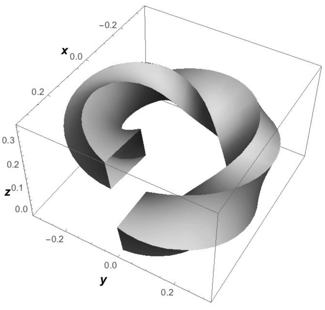
A solid rectangle with sides $d_{1}$ and $d_{2}$ can be parametrized by a map of type (4.1) by letting

where $-d_{1}/2\leq v\leq d_{1}/2$ and $-d_{2}/2\leq w\leq d_{2}/2$. We then have that

In this case we can compute the integrals in formula (3.6) to obtain (see Appendix 2 for details)

where

and

When there is no gyration, i.e. $\omega=0$, we have that

For $p=0$, this formula is the one obtained by Ogawa in [5].

In this case we have that

where the parameter $r$ is the radius of the circle used to construct the cardioidal curve. The interior of the region shown in the left part of Figure 4.4 is the region parametrized by the map $(v,w)\mapsto(\eta_{0}(v,w),\beta_{0}(v,w))$ for $0\leq v\leq 1$ and $-\pi\leq w\leq\pi$. The right part of the figure shows the channel resulting from gyrating this cross section over the Frenet-Serret frame of a helix. Under the above hypotheses we obtain

In this case, we use the series (3.10) to compute explicit formulas that approximate $\mathcal{D}$, and use numerical techniques to compute the integrals (3.6) in concrete examples.

We conclude by comparing the effective diffusion coefficients of the three types of twisted channels described above. To do a "fair" comparison we need to set the parameters of the cross sections so that their geometries are similar to second (geometric) order. We do this by equating their width functions $s_{1}$ and $s_{2}$ and their angle function $\theta$. For a fixed value of the parameter $r$ of the cardioid, the mayor and minor radii $r_{1}$ and $r_{2}$ of the elliptical cross section must be set to

and the sides $d_{1}$ and $d_{2}$ of the rectangular cross section must be set to

For the angle functions $\theta$ to be equal we simply need to use the same $\omega$ as the gyrating velocity in all cases.

We will illustrate the behaviour of the effective diffusion coefficients in these cases by letting

In Figure 4.6 we show the results obtained from the above selection of parameters by letting $r=1/20$, and in Figure 4.7 the results obtained by letting $r=1/15$. The effective diffusion formulas used in these examples are (4.3) and (4.4) for the elliptical and the rectangular case, and the cardioidal case was computed using numerical integration. To give an explanation of the behaviour just illustrated, we need the following description of the focal line.

The focal set of a 3-dimensional curve $\bm{\alpha}$ consists of the points of the form $\bm{\alpha}(u)+(1/\kappa(u))\hat{\bm{N}}(u)$. The focal line through such a point is the one having direction $\hat{\bm{B}}(u)$. The curve $\bm{\alpha}$ used in the examples in Figures 4.6 and 4.7 is a circle in the $xy$-plane with radius $a$, and in this case the focal set consists of the origin $(0,0,0)$ and the corresponding focal lines have direction $\hat{\bm{B}}=(0,0,1)$. For a given point $\bm{p}=\text{$\bm{\alpha}$}(u)+\eta(u,v,w)\hat{\bm{N}}(u)+\beta(u,v,w)\hat{\bm{B}}(u)$ in a cross section $S_{u}$, the distance of $\bm{p}$ to the corresponding focal line is

In order to simplify the arguments, let us assume that $<\eta>=0$ (which holds in our examples). Formula (3.6) can then be written as

Thus, we can make the following observations about the examples in Figures 4.6 and 4.7. The further away the cross section $S_{u}$ is from the focal line, the less influence the geometry (geometric moments information) of the cross section has on $\mathcal{D}(u)$. Notice that in Figure 4.6 the effective diffusion coefficients look more similar to each other than in Figure 4.7, where the effective diffusion coefficient for the rectangular channel has developed extra "bumps" due to the proximity of the channel to the focal line. As $r$ tends to $0$, the cross sections are further away from the focal line, and the effective diffusion coefficients look more similar to each other. In the limit when $r=0$, all the effective diffusion coefficients become equal to $D=1$.

We will now explain some of the features of the effective diffusion coefficients shown in Figures 4.6 and 4.7 in terms of the symmetries of the cross sections with respect to the normal field $\hat{\bm{N}}$. Observe that we have $0\leq u\leq\pi/2$ and $\omega=4$, so that the angle $\theta=\omega u$ covers a full cycle from $0$ to $2\pi$.

For $\theta=0,\pi/2,\pi,3\pi/2$ the ellipse is invariant under reflections with axis given by the normal vector $\hat{\bm{N}}$ at these points. This explains the four critical points of $\mathcal{D}$ at $u=0,\pi/8,\pi/4,3\pi/8$. When $u=0,\pi/4$ the mayor axis of the ellipse faces the focal line and the corresponding critical points are local maxima. When $u=\pi/8,3\pi/8$ the minor axis of the ellipse faces the focal line and the corresponding critical points are local minima. This is consistent with our observation that the closer the cross section is to the focal line, the larger the effect it has on the effective diffusion coefficient.

For $\theta=\pi/2,3\pi/2$ the cardioid is invariant under reflections with axis given by the normal vector $\hat{\bm{N}}$ at these points. This explains the two critical points of $\mathcal{D}$ at $u=\pi/8,3\pi/8$. These two points are local minima of $\mathcal{D}$, since the smallest axis of the cardioid faces the focal line for these angles. The first local minimum is smaller than the second because in the first case the "dent" of the cardioid is directed towards the focal line and in the second case this "dent" faces away from the focal line. The local maxima of $\mathcal{D}$ appearing near $u=0$ and $u=\pi/4$ can be explained again by the fact the largest axis of the cardioid faces the focal line at these angles, and the asymmetry of the the cardioid with respect to reflection along the normal line explains the fact that the $u$ values at which this maxima occur, appear with offsets (to the left and right) to the exact values $0$ and $\pi/4$.

The behaviour of the critical points in the rectangle case can be explained in a similar way as in the previous two cases, with the added effect (if the rectangle is close enough to the focal line) that the corners of the rectangle generate the "bumps" on the effective diffusion function (shown in Figure 4.7) as they get closer to the focal line.

References

- [1] P. Kalinay and K. Percus. Projection of a two-dimensional diffusion in a narrow channel onto the longitudinal dimension. The Journal of Chemical Physics, 122, 2005.
- [2] R.M. Bradley. Diffusion in a two-dimensional channel with curved midline and varying width. Phys. Rev. E, B 80, 2009.
- [3] L. Dagdug and I. Pineda. Projection of two-dimensional diffusion in a curved midline and narrow varying width channel onto the longitudinal dimension. The Journal of Chemical Physics, 137, 2012.
- [4] C. Valero and R. Herrera. Projecting diffusion along the normal bundle of a plane curve. Journal of Mathematical Physics, (5), 2014.
- [5] N. Ogawa. Diffusion in a curved cube. Physics Letters A, 377:2465–2471, 2013.
- [6] Anatoly E. Antipov, Alexander V. Barzykin, Alexander M. Berezhkovskii, Yurii A. Makhnovskii, Vladimir Yu. Zitserman, and Sergei M. Aldoshin. Effective diffusion coefficient of a brownian particle in a periodically expanded conical tube. Phys. Rev. E, 88:054101, Nov 2013.
- [7] M. Spivak. A Comprehensive Introduction to Differential Geometry, Vol II, volume 2. Publish or Perish, 1979.
- [8] M.P do Carmo. Differential Geometry of Curves and Surfaces. Prentice-Hall, 1976.