Fluorescence Correlation Spectroscopy and Nonlinear Stochastic Reaction-Diffusion
Abstract
The currently existing theory of fluorescence correlation spectroscopy (FCS) is based on the linear fluctuation theory originally developed by Einstein, Onsager, Lax, and others as a phenomenological approach to equilibrium fluctuations in bulk solutions. For mesoscopic reaction-diffusion systems with nonlinear chemical reactions among a small number of molecules, a situation often encountered in single-cell biochemistry, it is expected that FCS time correlation functions of a reaction-diffusion system can deviate from the classic results of Elson and Magde [Biopolymers (1974) 13:1-27]. We first discuss this nonlinear effect for reaction systems without diffusion. For nonlinear stochastic reaction-diffusion systems there are no closed solutions; therefore, stochastic Monte-Carlo simulations are carried out. We show that the deviation is small for a simple bimolecular reaction; the most significant deviations occur when the number of molecules is small and of the same order. Our results show that current linear FCS theory could be adequate for measurements on biological systems that contain many other sources of uncertainties. At the same time it provides a framework for future measurements of nonlinear, fluctuating chemical reactions with high-precision FCS. Extending Delbrück-Gillespie’s theory for stochastic nonlinear reactions with rapidly stirring to reaction-diffusion systems provides a mesoscopic model for chemical and biochemical reactions at nanometric and mesoscopic level such as a single biological cell.
1 Introduction
Single-molecule studies of biological macromolecules focus on conformational states of individual molecules and transitions between states [38, 5, 16, 32]. Concentration fluctuation spectroscopy, on the other hand, measures the molecular number fluctuations associated with linear, and nonlinear, biochemical reactions [9, 36]. For unimolecular reactions, these two approaches are conceptually equivalent, in statistical terms, via the multi-nomial distribution: If a single molecule has states with being the probability for the molecule in state at time , then for independent copies of the same molecule, one has the probability distribution for number of molecules in state following [20, 19]
| (1) |
where . In fact more specifically, if the first-order rate constant for transition is , then in the concentration fluctuation measurements of a system with independent copies of the molecule, the temporal correlation function is simply M times the correlation function derived from a single-molecule measurement. If we denote the “state of the reaction system” by , the rate constant for transition from to is . Experimentally, single-molecule measurements on state fluctuations have a much more superior signal-to-noise characteristics than the concentration fluctuation.
However, for reaction systems with nonlinear reactions such as , the two approaches no longer provide equivalent information; they are in fact complementary. This distinction has not been widely appreciated. Corresponding to chemistry reaction theories, the single-molecule approach parallels nicely with Kramers’ reaction rate theory [17], while the concentration fluctuation measurements is intimately related to Delbrück’s chemical master equation, or Gillespie’s stochastic kinetics, for chemical reaction systems with reaction networks [7, 13, 31]. In the latter systems, rate constants for individual reactions are supposely known a priori; complex chemical or biochemical behavior arises as a consequence of a nonlinear reaction network [32].
Fluorescence correlation spectroscopy (FCS) is one of the leading physiochemical techniques to experimentally measure concentration fluctuations of nonlinear chemical reactions with stochastic fluctuations in mesoscopic systems [33]. Other methods include conductance fluctuations for electrochemical reaction [11]. With the newfound perspective given above, especially with nonlinear chemical reactions in mind, we re-visit the original theory of FCS developed by Elson and Magde (EM) [10]. We show that the EM theory is based on the universally valid phenomenological linear approximation approach to macroscopic fluctuations, developed by Einstein for Brownian motion, Onsager and Machlup for linear Gaussian fluctuations [28], and Lax for nonequilibrium steady state [25]. A systematic exposition is given by Keizer[21]. The original EM theory was motivated by Eigen’s linear relaxation kinetics [12] and Onsager’s regression hypothesis [27]. It has been experimentally verified for concentration fluctuations in bulk solutions [26, 8].
There is a growing interest in the concentration
(or copy-number) fluctuation studies on single
live cells, both experimental [37]
and theoretical [31]. In this Letter,
we show that for some systems the linear,
phenomenological fluctuation theory breaks down, and
a mechanistic nonlinear stochastic reaction theory is
necessary.
Nonlinear chemical reaction. The nonlinear effect we discuss for FCS is also present in chemical relaxation kinetics. To illustrate this, consider the bimolecular reaction . According to Eigen’s theory, linear relaxation kinetics gives a single time constant :
| (2) |
The relaxation kinetics then is a single exponential for the concentration of : . However, the nonlinear kinetics based on the Law of Mass Action is
| (3) |
with
The term in the is due to the nonlinear effect. When the amplitude is sufficiently small, this term is negligible. Fig. 1 shows the fractional difference between the fully nonlinear relaxation kinetics given in (3) and the single exponential from the linear case. If the amplitude is small, the fractional difference will also be small and the linear approximation is valid; otherwise, there will be a significant difference between the linear and nonlinear case.
It is important to note that for nonlinear reactions the relaxation time not only depends on the individual rate constants, but also on the concentrations at equilibrium. Furthermore, for nonlinear reactions, the reaction rates depend on diffusion, as it’s clearly established in the theory of diffusion limited reactions [4, 6, 35]. Although not apparent in the Law of Mass Action, the diffusion is necessary to determine the macroscopic reaction rate. The coupling between the diffusion and the reaction rates is the actual source of the nonlinearity, and it is also the reason why the relaxation time depends on the composition at equilibrium. With this realization in mind, it becomes clear that the bimolecular association rate constant , and the diffusion constants for and used in EM theory are not independent parameters, see Appendix 5. It is worth to mention that in the MesoRD approach to stochastic reaction-diffusion, these parameters are treated as independent [18].
For stochastic reaction-diffusion kinetics, the difference between the linear and nonlinear systems can also be significant; however, the FCS systems are sufficiently complex and no analytical results are available. In order to address this issue, the present study will rely on Monte Carlo simulations to study nonlinear reaction-diffusion systems.
In Sec. 2, the implementation of an stochastic Monte Carlo method is explained. The parameters employed in the simulations are shown to be consistent with the ones used in EM theory. Sec. 3 shows the comparisons between the mesoscopic, nonlinear correlations obtained from Monte Carlo simulations and the EM theory. The discrepancies between these two are further discussed in section 4. For completeness, an appendix with the analytical results of the EM theory is included.
2 Simulation Methods
The results from the simulations performed in the present work will be compared to the results from EM theory [10]. Since some of the key molecular parameters used in the simulations are different from the “macroscopic” rate constants and diffusion coefficients in the EM theory, it is important that the parameters employed in the simulation are consistent with those from EM theory. We explain how the simulation was performed and show that the parameters are consistent.
Three-dimensional diffusion is simulated in terms of
3D random walk with time step, , and length step, .
These parameters are related to the 3D diffusion constants used in EM theory with or . The reason for different step sizes is to keep all the particles moving with a single frequency, which means, same time step and different diffusion coefficients. Initially, particles are positioned randomly with uniform distribution in a cubic box of dimensionless length 222 with periodic boundary conditions. There are three molecular species
represented by particles, , , and . At every time step, each particle moves with a distance of in one of
the , and directions at equal probability of
. Depending on if a reaction is involved, we have three cases to be discussed below in detail.
Pure diffusion. In this case, since reactions are not involved, there is only one specie (say ) of particles moving in a 3D random walk. In order to emulate FCS in simulation, we introduce a laser beam in the transverse plane with a cylindrical Gaussian intensity profile[9],
| (4) |
where is the intensity of the incident laser light at position , is the maximum intensity at the center of the beam and the focal volume is given by the radius at which . In the pure diffusion, as well as in all the other cases, the focal volume needs to be much smaller than the simulation box and considerably larger than the length step. In this case, setting the value of to the length step () as is sufficient for good accuracy. The fluctuation in the photocurrent is caused by the concentration fluctuation through
| (5) |
with,
Here, is the total number of particles and their positions. Therefore, the correlation of concentration fluctuations is just the temporal autocorrelation of the photocurrent, , calculated in the simulation as
| (6) |
where , starts from 0, and is the total number of time steps. is further normalized dividing by .
Note we are treating the molecules as point-like light sources; however, the molecular radii will be relevant when calculating the binding radius for the bimolecular reaction case.
Unimolecular isomerization. In this case, we consider a reaction of type with rate constants and , and an equilibrium constant . In the simulation, we set and as rate parameters of exponentially distributed waiting times. These are related to the probability of the reactions occurring via
respectively [13]. Without loss of generality, we assume particle and have the same diffusion coefficient and thereby the same characteristic length step . Once again, it’s sufficient to choose the focal volume . At each time step, besides of performing a random walk, particle can become with probability , and particle can become with probability . Concentration fluctuations for or are measured analogously to the pure diffusion case.
Bimolecular reaction. Some very effective and accurate methods have been developed for the bimolecular reaction with diffusion when the number of ligands is large [30, 29]. These are based on the analytical solution for the reversible diffusion-influenced reaction for an isolated pair in 1D and 3D [23, 1, 14, 24]. Unfortunately, the current work will require simulations in the nonlinear regime where we have a small number of ligands where these methods might not be appropriate. There are also other popular tools like the MesoRD and Smoldyn software to simulate these and other type of reactions [18, 3]; however, the simplicity of the simulations required allowed us to produce our own code employing a similar approach to Smoldyn[3].
Before addressing how to perfom the simulations for bimolecular reactions, note EM theory calculates the final autocorrelation function for the bimoleculer case as the sum of all the correlations weighted accordingly,
where is the correlation between molecule and , and can be or . The function contains the resulting photocurrent correlations from all the fluorescent molecules , and , including coupling effects. The autocorrelation function is the one that is actually compared to real experiments because it’s not experimentally possible to isolate the fluorescence of from that of the reaction product . However, in our computational setting, we can allow ourselves to concentrate on only one of these correlation curves, . This curve obtained from only the photocurrent fluctuations of molecule contains all the information we need, including both reaction rates. As EM theory should remain consistent, the error made when calculating the reaction rates by fitting the simulation correlation curve with the theoretical are equivalent to those made when fitting the experimental curve with the theoretical , with the exception of additional experimental errors. How to obtain the autocorrelation function that we will compare to our simulations is shown in the Appendix 5.
For the bimolecular simulations, the reaction is assumed to be with second-order rate constant (forward reaction rate), first-order rate constant (backward reaction rate) and equilibrium constant . Here, is the equilibrium concentration of specie . We assumed the diffusion coefficients to be and , since usually and are considered macromolecules and plays the role of a small ligand. Consequently, the lengths steps will obey , and a sufficiently accurate focal volume is found to be . Note the diffusion constant of a particle is not determined by its molecular weight per se but by its hydrodynamic radius. We set the probability of a backward reaction to occur in terms of the parameter as,
| (7) |
At every we check if any reaction occurs. For the forward reaction, we assume it’s diffusion limited. When the distance between molecules and is less than the binding radius , they react with probability one. The binding radius is given by the sum of the radii of and . Note that the binding radius should be much smaller than the focal volume , this condition is imposed in all the simulations. In the backward reaction, particle becomes and simply with probability . The newly formed molecule is placed where the molecule was, and the particle is placed a distance away from it in a random direction, with . If the particle happens to be placed inside the binding radius of another molecule, another random direction is chosen to avoid an artificial binding. The introduction of an unbinding radius is a possible solution to simulate the many-particle reaction accurately and address the issue of geminate recombinations in the diffusion limited model [3].
Note we called the backward rate and not . As particles and need to collide first before reacting, the effective forward rate required to compare to EM theory is unknown. Consequently, it is not clear if should be the effective backward rate either. Also note that for the bimolecular case, we do not expect the macroscopic concentrations relaxation to be exponential but a power law [15], this confirms that from equation (7) might not correspond to the effective backward rate . This is a subtle matter that will be treated in an upcoming manuscript. For the purpose of the current work, understanding some of the dynamics of geminate recombinations[2, 22] will help us address this issue.
Geminate recombinations. Geminate recombinations occur when a particle that just dissociated from a certain , associates again with it[22, 2, 3]. At first sight, it is not evident how this phenomena alters the reaction rates. One way to understand it is in terms of the waiting times. For the first reaction, the molecule is positioned randomly with a uniform distribution outside of the reaction sphere of radius . The mean first passage waiting time for the reaction to occur is the one given by Collins and Kimball’s or Smoluchowski’s theory[6, 34]. However, whenever a dissociation occurs, the particle is always positioned very near . As a result, the distribution of the initial position of the molecule should not be uniform, and the average waiting time for the forward reaction to occur again will no longer be the one given by Collins and Kimball or Smoluchowski’s theory. As the average waiting times and the rates are inversely proportional, the effective forward rate cannot be expected to be the same either [35, 34]. In other words, the just dissociated has a higher chance to bind to the same . This is conceptually prevented in the classical Law of Mass Action, and Delbruck-Gillespie theory, which require a rapid stirring reaction vessel [13].
So how to map the correct forward rate to EM theory? Let us focus on the Smoluchowski approach and call the probability of a geminate recombination to occur. In a system in equilibrium with several molecules, the law of large numbers tells us that a fraction of all the forward reactions are due to geminate recombinations. Therefore, we expect that the remaining fraction follows the forward reaction rate for irreversible reactions given by Smoluchowski’s theory. This yields the relation between the irreversible rate of Smoluchowski[6], with , and the reversible effective forward rate as[3]
| (8) |
In order to calculate the backward rate, we only need to know the equilibrium constant . From our simulation, we can calculate it in terms of the average concentrations as . However, we also know , so the effective backward rate can be calculated as
| (9) |
The only question left to answer is how to calculate the probability of geminate recombinations . As geminate recombinations are actually an stochastic process, there are many issues to deal with in order to fully address that question. A separated manuscript regarding some of these is in preparation. However, a simple approach using Smoluchowski’s original solution with an unbinding radius will be sufficient for our current purpose[3]. We can solve Smoluchowski’s steady state equation for a reversible reaction in equilibrium using an absorbing boundary condition at and a constant concentration at [3]. These boundary conditions mean that the flux at the source equals the flux at the sink in , as it’s expected from a reversible reaction at equilibrium. The solution to this boundary problem is given by
where can be understood as the concentration of or as the radial distribution function if it’s normalized. The reaction rate is given by the flux, per average concentration of molecules, ,
| (10) |
Note that as the original Smoluchowski’s irreversible rate is recovered. Comparing this result with equation (8) yields that [3]. It’s important to note this analytic result is only fully valid in the limit of infinitely accurate Brownian Motion. In our simulation, we’ll employ random walks with very small characteristic length step, so equation (10) is a good approximation of the forward rate. If the characteristic step is increased, the simulations become faster; however, a more complicated approach is necessary to calculate the correct reaction rates, as the one used by Smoldyn software[3]. For the purpose of this work, computational efficiency is not an immediate issue, so we employ characteristic length steps that are small enough to use the forward rate given in equation (10) accurately.
It is still not evident how to choose the appropriate unbinding radius . An initial guess satisfying is made. Since every different unbinding radius yields different values of the forward rate, the final concentrations at equilibrium and the equilibrium constant , the simulation is executed to yield these for the initial guess. Afterwards, the unbinding radius is recalculated in terms of the final concentrations, and the process is repeated until the unbinding radius remains practically constant between iterations. The unbinding radius in each iteration is recalculated as,
| (11) |
where is the volume of the cubic box and is the number of particles at equilibrium. This expression is obtained by assuming each molecule has it’s own mini-sphere with volume . In this sphere we can assume the behavior is the same as in Smoluchoski’s theory which involves only one copy of the molecule. Assuming is positioned at the center of the sphere , the appropriate unbinding radius would correspond to the distance between and the border of the sphere. This value is clearly given by expression (11).
Once the unbinding radius is calculated, is determined as well as the forward rate . The effective backward rate is obtained with and the equilibrium constant using equation (9). These last three parameters are precisely the ones used in EM theory [10]. In order to validate the simulation, we tested the case with one molecule fixed at the center. The forward rate was calculated using the average first passage time after each forward reaction [35, 34] from the simulation and the Smoluchowski equation for reversible reaction (10). The relative error between the two calculated forward rates was less than five percent for 100 runs with time iterations. These results provide consistency between the parameters used in our simulation and the parameters from EM theory.
3 Results
As controls, both pure diffusion and unimolecular reaction with diffusion are carried out first. The EM theory for both these linear stochastic dynamics is exact; hence, it is expected to agree completely with the simulations, aside from statistical uncertainties. This is indeed the case as shown in Figs. (2a) and (3a).
For the nonlinear reaction with diffusion, EM theory has no exact solution; however, linearization around equilibrium yields a correlation curve in the form of an integral. This integral can be approximated asymptotically for certain range of parameters, or it can be solved numerically. For details on the analytic solutions, see the Appendix 5. For certain values of the equilibrium concentration, the simulation deviates from these solutions. We account this deviation to the non-linear effects that are present in the simulation but not in EM theory. The maximum errors are calculated with the maximum norm, which for the error between and is given by .
To ensure the validity of the results, two asymptotic
limits, where the nonlinear effects are known to be negligible, are employed as a third and fourth control. In order to provide a quantification of the non-linear deviation, its magnitude is studied as a function of the forward reaction rate and the number of molecules.
All these will be further discussed in detail.
Control I: pure diffusion.
The calculated , normalized autocorrelation
function, from simulations with the number of particles, , and total measurement time, , is
plotted along the analytical solution in Fig. (2a). Aside from statistical errors, the simulation results
agree completely with the analytical solution (12) as expected. We further calculate the difference between the analytical solution and the simulation results with different total measurement time, as depicted in Fig. (2b). Consistently, it shows that this difference is decreasing with increasing total measurement time . Note that since particles are treated independently, an increase in the total measurement time is equivalent to increasing the number of particles.
Control II: unimolecular reaction with diffusion.
Analogously to the pure diffusion case, we calculate the temporal autocorrelation of the photocurrent, , for either species of particles. Without loss of generality, we choose the initial number of and particles equal, i.e. . We calculate the photocurrent for particle along with the analytic solution (14), as plotted in Fig. (3a). The simulation results are again in good agreement with the analytic solution. In addition, we calculate the difference between the analytical solution and simulation results of for different total measurement times. As depicted in Fig. (3b), the error between the analytical result and the simulation decreases as the total measurement time increases. Once more, as the particles react independently of each other, an increase in the total measurement time is equivalent to increasing the number of particles evenly.
Nonlinear reaction with diffusion.
We choose and small and of the same order. We calculate the temporal autocorrelation of the photocurrent for particle and compare it against the analytical solution. In Fig. (4a) two solutions for the correlation curve are shown: the simulation curve and the numerical approximation of the analytic solution integral (15). As and are of the same order, the asymptotic approximation of the integral is outside its range of validity (see Appendix 5), and it’s not included in the plot. A noticeable disagreement between the simulation and the numerical analytic integration result is observed as depicted in Fig. (4a). The maximum error between the simulation and the analytic solution is around , and the theory will produce an error of in the forward reaction rate if fitted to the central tendency in the simulation curve. The plots in Figs. (4b) and (4c) correspond to the two asymptotic limits where the nonlinear effects are negligible and the simulation converges to the analytic linear theory. These two limits will be discussed next.

Asymptotic limit I: large number of ligands. In the case where , the concentration of molecules barely fluctuates. Consequently, the nonlinear reaction with diffusion approaches asymptotically a linear unimolecular reaction with diffusion, i.e. the nonlinear effects are negligible. A simple example is given by the law of mass action for . If barely fluctuates around , the concentration of follows
with the concentrations of and the second order rate constant.
The last equation is clearly linear and EM theory provides an exact result for it. In Fig. 5, besides the same two solutions as plotted before, the exact analytic solution approached as becomes is also included. Since it’s in its range of validity and the non-linear effects are negligible, the asymptotic approximation of the linear analytic solution (15) is also plotted. The four solutions, including the simulation and the numerical integration of (15), converge to the same correlation curve, as expected. This result is clearly depicted in Fig. 5. It also shows consistency with our two controls, since the error decreases when increasing the number of particles. Recovering the correct asymptotic limit when serves as a third control to validate our simulation.
Asymptotic limit II: large number of all molecules.
If the number of all the molecules is increased, i.e. , the concentration of any of the species barely fluctuates around equilibrium. Analogously to
the previous case, the nonlinear effects become second order and the system approaches a linear solution, which is plotted as the exact analytic solution in Fig. 6. Additionally, the numerical analytic solution and the simulation curves are plotted as before. In this case, the asymptotic approximation of the linear analytic solution (15) is not in its range of validity, so it is not included. As we can see in Fig. 6, the simulation, the numerical analytic solution and the exact linear unimolecular solution are all converging, i.e. the non-linear effects are becoming negligible as the number and is increased. This asymptotic limit serves as a fourth control to validate the simulation.
Nonlinear deviation variation. In order to better quantify the deviation for the nonlinear reaction case shown in Fig. 4. We calculated how this deviation varies in term of the relative change in the forward reaction rate (Fig. 7) and with the uniform increase in the number of all molecules (Fig. 7).
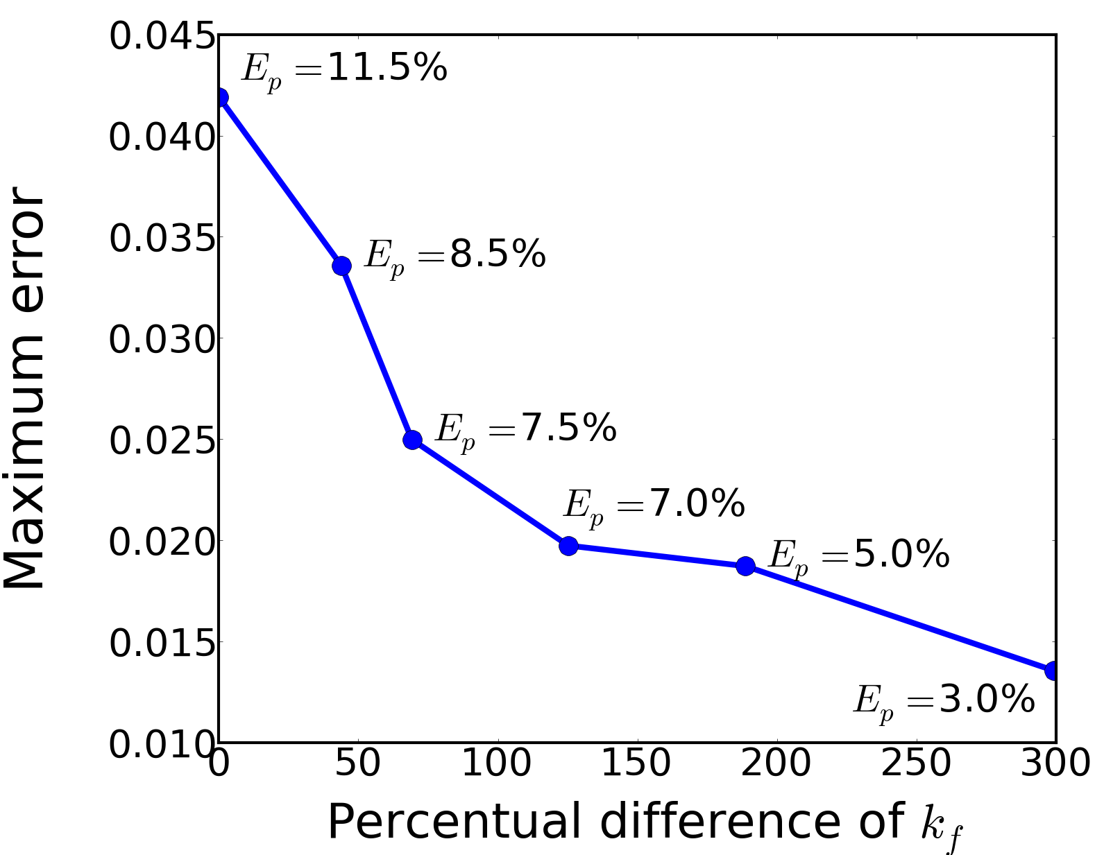

The plot shown in Fig. 7 shows the convergence to the asymptotic limit II: Large number of all molecules. As expected from our previous result, the error is gradually reduced as the number of all molecules is increased. Furthermore, on the plot in Fig. 7, we manipulated the forward reaction rates . As these rates are related to the diffusion coefficients by equation (10), the best way to manipulate the reaction rate is to modify the characteristic length step . In this case we multiplied (with ) by a constant between one and two, which yields a percentage variation of the forward reaction rate up to .
The deviation in Fig. 7 is reduced as the reaction rate is increased. This is expected from the law of mass action for , where their concentrations and satisfy in the steady state. In this expression it is clear how an increase in the forward rate can be equivalent to an increase of . Consequently this case is equivalent to the asymptotic limit I: large number of ligands. As the characteristic length step is increased, the error by approximating diffusion by a random walk is also increased. However, this error is still not relevant as the overall error shown in Fig. 7 decays as the reaction rate is increased.
Also note each point in Fig. 7 has an associated percentual error, . This was obtained by testing slightly different values for the forward rate in the analytic curve until the maximum error against the simulation was below . Ideally a least squares fitting could be employed. However, we are currently developing a faster and more robust simulation to illustrate a complete landscape of the deviations as a function of two or more parameters, which will include a least square fitting to obtain the percentual error. The results will be provided in an upcoming manuscript.
4 Discussion
We showed that our simulation recovers the correct reaction rates of the Smoluchowski’s model for reversible reactions providing consistency between the simulation parameters and the parameters used by EM theory. As first controls, the exact solutions of EM theory for the pure diffusion and the unimolecular reaction with diffusion were recovered by our simulation. In addition, to further validate the simulation, two asymptotic limits were tested. In the asymptotic limits of large number of ligands and large number of molecules, the simulation and the theoretical correlation curves converge as expected. This confirms that in these limits the nonlinear effects become negligible and linear EM theory is very accurate. However, in the case where and are not very big and have similar values (around 35 each), we showed the simulation results deviate from those of linear EM theory. As the simulation proved to be an accurate model, we account the deviations due to nonlinear effects that are depreciated in linear EM theory[9], as briefly shown in the Appendix 5.
The dependance of the deviation in the number of molecules and the reaction rates was analyzed. When employing an increasing number of all of the molecules, we observe the deviation is reduced and the system gradually reaches the asymptotic limit II, as expected. When the forward reaction rate was gradually increased up to its original value, we again observe the error is reduced. This is due the fact that increasing the reaction rate produces a similar effect to that of the increase in the number of ligands, which corresponds to the asymptotic limit I, where the error is also reduced.
For most experimental scenarios the assumptions or are appropriate, and the results provided by EM theory are very accurate. Nonetheless, the present paper showed that when the number of molecules is small, nonlinear effects are not negligible showing a deviation between the simulation of the nonlinear model and linear EM theory. However, experimental FCS correlation curves usually involve other sources of noise not considered in the simulated fluctuations, like mismatch of refractive indexes and photobleaching of fluorophores amongst others. As we found the deviation to be small with a error in the reaction rates, it is likely that the error produced by the nonlinearity is still within the experimental uncertainty of current laboratory measurements, so it might require a more carefully designed setup and clean system to test our theory.
In particular, we do not believe the nonlinear effect will be relevant in the current cellular biophysical investigations. Rather, the significance of the present work is to bring quantitative experimental measurements on nanometric, nonlinear chemical reactions a step closer to a stochastic theoretical framework. It also intends to call attention to nonlinear kinetics in the fluctuation chemistry setting. Certainly, we hope this work paves the way to study more complex nonlinear reactions with concentration fluctuations. We are certain for other more complex reaction systems the nonlinear effect can be larger. Furthermore, on the practical side, nonlinear chemical reactions in biology are widely present; so being able to show, at least in the simplest case, the EM theory works well, even in a context where nonlinearities are significant, is a relevant contribution for currenct practice of FCS in biochemistry.
With the increasing accuracy and ability of single-molecule techniques, results like the ones obtained herein will become experimentally accessible. We also believe FCS will grow more and more into an analytical tool. In a clear analytical chemistry setting, an deviation would be significant . It is true that such level of quantification is still in development; but we hope results like ours provide additional motivation. Developing nonlinear chemical reaction theory with fluctuations, in terms of FCS or more generally speaking, remains a challenge.
5 Appendix: EM theory analytic results
Three main results from EM theory [9] are incorporated in this appendix. For the three cases, pure diffusion, unimolecular isomerization and nonlinear reaction with diffusion, the full expressions for the correlation curves are given. Additional details are given to explain why EM theory is a linear theory for the bimolecular reaction.
The parameters used are the time step, with or
the diffusion length step for every time step taken, the diffusion coefficient of
and focal volume given by the radius of the Gaussian laser.
Pure diffusion. The normalized auto correlation curve for purely diffusive molecules is given by,
| (12) | |||
| (13) |
Unimolecular reaction with diffusion. The normalized autocorrelation curve of for the diffusive reaction with is given by,
| (14) |
with , and,
Nonlinear reaction with diffusion. The normalized autocorrelation curve of for the diffusive reaction with is given by the integral,
| (15) |
with
where and are the Fourier frequency variables corresponding to the spatial variables and . The integral cannot be solved exactly; nonetheless, we have two possible approaches: provide an asymptotic approximation or solve it numerically. The former, as done in EM theory[9], requires that and . The numerical solution doesn’t require any of these conditions. In section (3), we employ both approaches to compare the theory against our simulation.
In equation (15), is given by
| (16) |
with or . The quantities for are the right eigenvectors, are the left eigenvectors and are the three eigenvalues of matrix from (18). The matrix is obtained from the reaction diffusion equation for the concentration of the three molecules at position r and time . The concentration for the three molecules will be given by the vector with components and or . The full nonlinear reaction diffusion equation is given by
| (17) |
where D is a diagonal matrix with the chemical diffusion coefficients , and M is the stoichiometry matrix11 1 Matrix of reaction coefficients based on the Law of Mass action.. Note that M is not a constant coefficient matrix, since this is a nonlinear reaction, it depends on the concentration vector . Supposing the system is stationary, the chemical concentrations will reach a thermodynamic equilibrium; therefore, the mean concentration of each component will be given by the ensemble average of the concentration, i.e. . The ensemble average can be understood as the averaged quantity over many identical systems at a certain time. Although the partial differential equation (PDE) (17) is deterministic, another linear PDE can be derived for the fluctuations of the system around equilibrium. This fluctuations will be given by . Substituting into (17) and dropping the nonlinear terms we obtain the PDE for the fluctuations
| (18) |
where the constant coefficient matrix
with .
Acknowledgements
We thank helpful discussions with Drs. Noam Agmon, Steve Andrews, Attila Szabo, and Nancy Thompson. The authors would also like to thank two anonymous reviewers who greatly improved the quality of this paper. MJdR acknowledges partial support from National Science and Technology Council of Mexico (CONACyT). HQ acknowledges partial support from Pacific Northwest National Laboratory (PNNL) subcontract PR 203607. W.P. and G.L. acknowledge the funding support by the Applied Mathematics Program within the U.S. Department of Energy Office of Advanced Scientific Computing Research as part of the Collaboratory on Mathematics for Mesoscopic Modeling of Materials (CM4), under award number DE-SC0009247. PNNL is operated by Battelle for the DOE under Contract DE-AC05-76RL01830.
References
- [1] Agmon, N. Diffusion with back reaction. J. Chem. Phys 81, 6 (1984), 2811–2817.
- [2] Agmon, N., and Szabo, A. Theory of reversible diffusion-influenced reactions. J. Chem. Phys 92, 9 (1990), 5270–5284.
- [3] Andrews, S. S., and Bray, D. Stochastic simulation of chemical reactions with spatial resolution and single molecule detail. PB 1, 3 (2004), 137.
- [4] Berg, O. G. On diffusion-controlled dissociation. Chem. Phys. 31, 1 (1978), 47–57.
- [5] Bustamante, C. In singulo biochemistry: When less is more. Annu. Rev. Biochem. 77 (2008), 45–50.
- [6] Collins, F. C., and Kimball, G. E. Diffusion-controlled reaction rates. J. Colloid Sci. 4, 4 (1949), 425–437.
- [7] Delbrück, M. Statistical fluctuations in autocatalytic reactions. J. Chem. Phys 8, 1 (1940), 120–124.
- [8] Ehrenberg, M., and Rigler, R. Rotational brownian motion and fluorescence intensify fluctuations. Chem. Phys. 4, 3 (1974), 390–401.
- [9] Elson, E., and Webb, W. Concentration correlation spectroscopy: a new biophysical probe based on occupation number fluctuations. Annu. Rev. Biophys. 4, 1 (1975), 311–334.
- [10] Elson, E. L., and Magde, D. Fluorescence correlation spectroscopy. i. conceptual basis and theory. Biopolymers 13, 1 (1974), 1–27.
- [11] Feher, G., and Weissman, M. Fluctuation spectroscopy: Determination of chemical reaction kinetics from the frequency spectrum of fluctuations. Proc. Natl. Acad. Sci. U.S.A. 70, 3 (1973), 870–875.
- [12] Friess, S. Technique of organic chemistry, vol. viii, part ii: Investigation of rates and mechanisms of reactions. interscience, new york, 1963; m. eigen, l. de mayer, relax. Methods, 895–1054.
- [13] Gillespie, D. T. Stochastic simulation of chemical kinetics. Annu. Rev. Phys. Chem. 58 (2007), 35–55.
- [14] Gopich, I. V., Solntsev, K. M., and Agmon, N. Excited-state reversible geminate reaction. i. two different lifetimes. J. Chem. Phys 110, 4 (1999), 2164–2174.
- [15] Gopich, I. V., and Szabo, A. Kinetics of reversible diffusion influenced reactions: the self-consistent relaxation time approximation. J. Chem. Phys 117, 2 (2002), 507–517.
- [16] Gräslund, A., Rigler, R., and Widengren, J. Single Molecule Spectroscopy in Chemistry, Physics and Biology. Springer, 2010.
- [17] Hänggi, P., Talkner, P., and Borkovec, M. Reaction-rate theory: Fifty years after kramers. Rev. Mod. Phys. 62, 2 (1990), 251.
- [18] Hattne, J., Fange, D., and Elf, J. Stochastic reaction-diffusion simulation with mesord. Bioinformatics 21, 12 (2005), 2923–2924.
- [19] Hill, T. L. Approach of certain systems, including membranes, to steady state. J. Chem. Phys 54, 1 (1971), 34–35.
- [20] Hill, T. L., and Plesner, I. W. Studies in irreversible thermodynamics. ii. a simple class of lattice models for open systems. J. Chem. Phys 43, 1 (1965), 267–285.
- [21] Keizer, J. Statistical Thermodynamics of Nonequilibrium Processes. Springer, 1987.
- [22] Khokhlova, S. S., and Agmon, N. Comparison of alternate approaches for reversible geminate recombination. Bull. Korean Chem. Soc 33, 3 (2012), 1021.
- [23] Kim, H., and Shin, K. J. Exact solution of the reversible diffusion-influenced reaction for an isolated pair in three dimensions. Phys. Rev. Lett. 82 (1999), 1578–1581.
- [24] Kim, H., Shin, K. J., and Agmon, N. Excited-state reversible geminate recombination with quenching in one dimension. J. Chem. Phys 111, 9 (1999), 3791–3799.
- [25] Lax, M. Fluctuations from the nonequilibrium steady state. Rev. Mod. Phys. 32, 1 (1960), 25.
- [26] Magde, D., Elson, E., and Webb, W. W. Thermodynamic fluctuations in a reacting system—measurement by fluorescence correlation spectroscopy. Phys. Rev. Lett. 29 (Sep 1972), 705–708.
- [27] Onsager, L. Reciprocal relations in irreversible processes. ii. Phys. Rev. 38, 12 (1931), 2265.
- [28] Onsager, L., and Machlup, S. Fluctuations and irreversible processes. Phys. Rev. 91, 6 (1953), 1505–1512.
- [29] Popov, A. V., and Agmon, N. Three-dimensional simulation verifies theoretical asymptotics for reversible binding. Chem. Phys. Lett. 340, 1 (2001), 151–156.
- [30] Popov, A. V., and Agmon, N. Three-dimensional simulations of reversible bimolecular reactions: The simple target problem. J. Chem. Phys 115, 19 (2001), 8921–8932.
- [31] Qian, H. Cellular biology in terms of stochastic nonlinear biochemical dynamics: Emergent properties, isogenetic variations and chemical system inheritability. J. Stat. Phys. 141, 6 (2010), 990–1013.
- [32] Qian, H., and Kou, S. Statistics and related topics in single-molecule biophysics. Annu. Rev. Statstics 1 (2014), 465–492.
- [33] Rigler, R., and Elson, E. e. Fluorescence Correlation Spectroscopy: Theory and Applications. Springer Series in Chemical Physics, vol. 65, New York, 2001.
- [34] Shoup, D., and Szabo, A. Role of diffusion in ligand binding to macromolecules and cell-bound receptors. Biophys. J. 40, 1 (1982), 33–39.
- [35] Szabo, A., Schulten, K., and Schulten, Z. First passage time approach to diffusion controlled reactions. J. Chem. Phys 72, 8 (1980), 4350–4357.
- [36] Weissman, M. B. Fluctuation spectroscopy. Annu. Rev. Phys. Chem. 32, 1 (1981), 205–232.
- [37] Xie, X. S., Choi, P. J., Li, G.-W., Lee, N. K., and Lia, G. Single-molecule approach to molecular biology in living bacterial cells. Annu. Rev. Biophys. 37 (2008), 417–444.
- [38] Xie, X. S., and Trautman, J. Single-molecule optical studies at room temperature. Annu. Rev. Phys. Chem 49 (1998), 441–480.