An error correcting parser for context free grammars
that takes less than cubic time
Abstract
The problem of parsing has been studied extensively for various formal grammars. Given an input string and a grammar, the parsing problem is to check if the input string belongs to the language generated by the grammar. A closely related problem of great importance is one where the input are a string and a grammar and the task is to produce a string that belongs to the language generated by and the ‘distance’ between and is the smallest (from among all the strings in the language). Specifically, if is in the language generated by , then the output should be . Any parser that solves this version of the problem is called an error correcting parser. In 1972 Aho and Peterson presented a cubic time error correcting parser for context free grammars. Since then this asymptotic time bound has not been improved under the (standard) assumption that the grammar size is a constant. In this paper we present an error correcting parser for context free grammars that runs in time, where is the length of the input string and is the time needed to compute the tropical product of two matrices.
In this paper we also present an -approximation algorithm for the language edit distance problem that has a run time of , where is the time taken to multiply two matrices. To the best of our knowledge, no approximation algorithms have been proposed for error correcting parsing for general context free grammars.
1 Introduction
Parsing is a well studied problem owing to its numerous applications. For example, parsing finds a place in programming language translations, description of properties of semistructured data [12], protein structures prediction [11], etc. For context free grammars, two classical algorithms can be found in the literature: CYK [3, 14, 6] and Earley [4]. Both of these algorithms take time in the worst case. Valiant has shown that context free recognition can be reduced to Boolean matrix multiplication [13].
The problem of parsing with error correction (also known as the language edit distance problem) has also been studied well. Aho and Peterson presented an time algorithm for context free grammar parsing with errors. Three kinds of errors were considered, namely, insertion, deletion, and substitution. This algorithm depended quadratically on the size of the grammar and was based on Earley parser. Subsequently, Myers [9] presented an algorithm for error correcting parsing for context free grammars that also runs in cubic time but the dependence on the grammar size was linear. This algorithm is based on the CYK parser.
As far as the worst case run time is concerned, to the best of our knowledge, cubic time is the best known for the error correcting parsing problem for general context free grammars. A number of approximation algorithms have been proposed for the DYCK language (which is a very specific context free language). See e.g., [12].
In this paper we present a cubic time algorithm for error correcting parsing that is considerably simpler than the algorithms of [1] and [9]. This algorithm is based on the CYK parser. Even though the algorithm of [9] is also based on CYK parser, there are some crucial differences between our algorithm and that of [9]. We also show that the language edit distance problem can be reduced to the problem of computing the tropical product (also known as the distance product or the min-plus product) of two given matrices where . Using the current best known run time [2] for tropical matrix product, our reduction implies that the language edit distance problem can be solved exactly in time, improving the cubic run time that has remained the best since 1972.
In many applications, it may suffice to solve the language edit distance problem approximately. To the best of our knowledge, no approximation algorithms are known for general context free grammars. However, a number of such algorithms have been proposed for the Dyck language. Dyck language is a basic and fundamental context free grammar and the Dyck language edit distance is a significant generalization of string edit distance problem which has been widely studied. Also, the non-deterministic Dyck language is the hardest context free grammar in terms of parsing. The concept of approximate error correcting parsing was introduced by [7]. The algorithm of [7] takes subcubic time but its approximation factor is . If is a string in the language generated by the input grammar that has the minimum language edit distance (say ) with the input string and if an algorithm outputs a string such that the language edit distance between and is no more than , then we say that is a -approximation algorithm. Saha [12] gives the very first near-linear time algorithm for Dyck language edit distance problem with polylog approximaiton and an time algorithm with approximation where is the edit distance. [12] not only studies Dyck language edit distance problem, but also a larger class of problems including the memory checking languages, which comprise of transcripts of any popular data structure. It can also be applied to other variants of languages studied by Parnas, Ron and Rubinfeld (APPRO-RANDOM, 2001). It is noteworthy that Dyck grammar parsing (without error correction) can easily be done in linear time. On the other hand, it is known that parsing of arbitrary context free grammars is as difficult as boolean matrix multiplication [8]. For an extensive discussion on approximation algorithms for the Dyck language, please see [12]. In this paper we present an approximation algorithm for general context free grammars. Specifically, we show that if we are only interested in edit distances of no more than , then the language edit distance problem can be solved in time where ) is the time taken to multiply two matrices. (Currently the best known value for is 2.376). As a corollary, it follows that there is an -approximation algorithm for the language edit distance problem with a run time of .
1.1 Some Notations
A context free grammar is a 4-tuple , where is a set of characters (known as terminals) in the alphabet, is a set of variables known as nonterminals, is the start symbol (that is a nonterminal) and is a set of productions.
We use to denote the language generated by . Capital letters such as will be used to denote nonterminals, small letters such as will be used to denote terminals, and greek letters such as will be used to denote any string from .
A production of the form is called an -production. A production of the kind is known as a unit production.
Let be a CFG such that does not have . Then we can convert into Chomsky Normal Form (CNF). A context free grammar is in CNF if the productions in are of only two kinds: and .
Let and be two real matrices. Then the tropical (or distance) product of and is defined as: .
The edit distance between two strings and from an alphabet is the minimum number of (insert, delete, and substitution) operations needed to convert to .
In this paper we assume that the grammar size is which is a standard assumption made in many works (see e.g., [13]).
1.2 Some Preliminaries
1.2.1 A summary of Aho and Peterson’s algorithm
The algorithm of Aho and Peterson [1] is based on the parsing algorithm of Earley [4]. There are some crucial differences. Let be the input string. If is the input grammar, another grammar is constructed where has all the productions of and some additional productions that can be used to make derivations involving errors. Each such additional production is called an error production. Three kinds of errors are considered, namely, insertion, deletion, and substitution. also has some additional nonterminals. The algorithm derives the input string beginning with , minimizing the number of applications of the error productions.
The parser of [1] can be thought of as a modified version of the Earley parser. Like the algorithm of Earley, levels of lists are constructed. Each list consists of items where an item is an object of the form . Here is a production, . is a special symbol that indicates what part of the production has been processed so far, is an integer indicating input position at which the derivation of started, and is an integer indicating the number of error productions that have been used in the derivation from . If we use to denote the list of level , then the item will be in if and only if for some in , and using error productions.
The algorithm constructs the lists . An item of the form will be in , for some integer . In this case, is the minimum edit distance between and any string in .
Note that the Earley parser also works in the same manner except that an item will only have two elements: .
1.2.2 A synopsis of Valiant’s algorithm
Valiant has presented an efficient algorithm for computing the transitive closure of an upper triangular matrix. The transitive closure is with respect to matrix multiplication defined in a specific way. Each element in a matrix will be a set of items. In the case of context free recognition, each matrix element will be a set of nonterminals. If and are two sets of nonterminals, a binary operator is defined as: such that . If and are matrices where each element is a subset of , the product matrix of and is defined as follows.
Under the above definition of matrix multiplication, we can define transitive closure for any matrix as:
where and
Valiant has shown that this transitive closure can be computed in time, where is the time needed for multiplying two matrices with the above special definition of matrix product. In fact this algorithm works for the computation of transitive closure for generic operators and union as long as these operations satisfy the following properties: The outer operation (i.e., union) is commutative and associative, the inner operation () distributes over union, is a multiplicative zero and an additive identity.
2 A Simple Error Correcting Parser
In this section we present a simple error correcting parser for CFGs. This algorithm is based on the algorithm of [10]. We also utilize the concept of error productions introduced in [1]. If is the input grammar, we generate another grammar where . has all the productions in . In addition, has some additional error productions. We parse the given input string using the productions in . For each production, we associate an error count that indicates the minimum number of errors the use of the production will amount to. The goal is to parse using as few error productions as possible. Specifically, the sum of error counts of all the error productions used should be minimum. If is an error production with an error count of , we denote this rule as . If there is no integer above in any production, the error count of this production should be assumed to be .
2.1 Construction of a covering grammar
Let be the given grammar and be the given input string. Without loss of generality assume that does not have and that is in CNF. Even if is not in CNF, we could employ standard techniques to convert into this form (see e.g., [5]). We construct a new grammar as follows. has the following productions in addition to the ones in : , , and for every . Here and are new nonterminals. If is in , then add the following rules to : for every , , , and . Each production in has an error count of .
Elimination of -productions: We first eliminate the -productions in as follows. We say a nonterminal is nullable if . Let be the number of errors needed for to derive . We denote this as follows: . Call the of , denoted as . We only keep the minimum such for any nonterminal. Let the minimum for any terminal be . For example, if , and are in , then . We identify all the nullable nonterminals in using the following procedure. If is in and if both and are nullable, then is nullable as well. In this case, .
After identifying all nullable nonterminals and their values, we process each production as follows. Let be any production in . If is nullable and is not, and if , then we add the production to . If is nullable and is not, and if , then we add the production to . If both or none of and are nullable, then we do not add any additional production to while processing the production . If there are more than one productions in with the same precedent and consequent, we only keep that production for which the error count is the least.
Finally, we remove all the productions.
Elimination of unit productions: We eliminate unit productions from as follows. Let be a sequence of unit productions in and be a non unit production. In this case we add the production to , where . After processing all such sequences and adding productions to we eliminate duplicates. In particular, if there are more than one rules with the same precedent and consequent, we only keep the production with the least error count. At the end we remove all the unit productions.
Observation: Aho and Peterson [1] indicate that is a covering grammar for and prove several properties of . Note that they don’t keep any error counts with their productions. Also, the validity of the procedures we have used to eliminate and unit productions can be found in [5].
An Example. Consider the language . A CFG for this language has the productions: . We can get an equivalent grammar in CNF where and .
We can get a grammar with error productions where , and . Note that any production with no integer above has an error count of zero.
- •
Eliminating -productions: We identify nullable nonterminals. We realize that the following nonterminals are nullable: , and . For example, is nullable since we have: . We also realize: , and .
Now we process every production in and generate new relevant rules. For instance, consider the rule . Since , we add the rule to . When we process the rule , since , we realize that has to be added to . However, has already been added to . Thus we replace with .
Processing in a similar manner, we add the following productions to to get : , , and . We eliminate all the -productions from .
- •
Eliminating unit productions: We consider every sequence of unit productions in with being a non unit production. In this case we add the production to , where .
Consider the sequence . This sequence results in a new production: . The sequence suggests the addition of the production . But we have already added a better production and hence this production is ignored.
Proceeding in a similar manner we realize that we have to add the following productions to to get : , , , , , , , , , , , , , and . We eliminate all the unit productions from .
The final grammar we get is where .
2.2 The algorithm
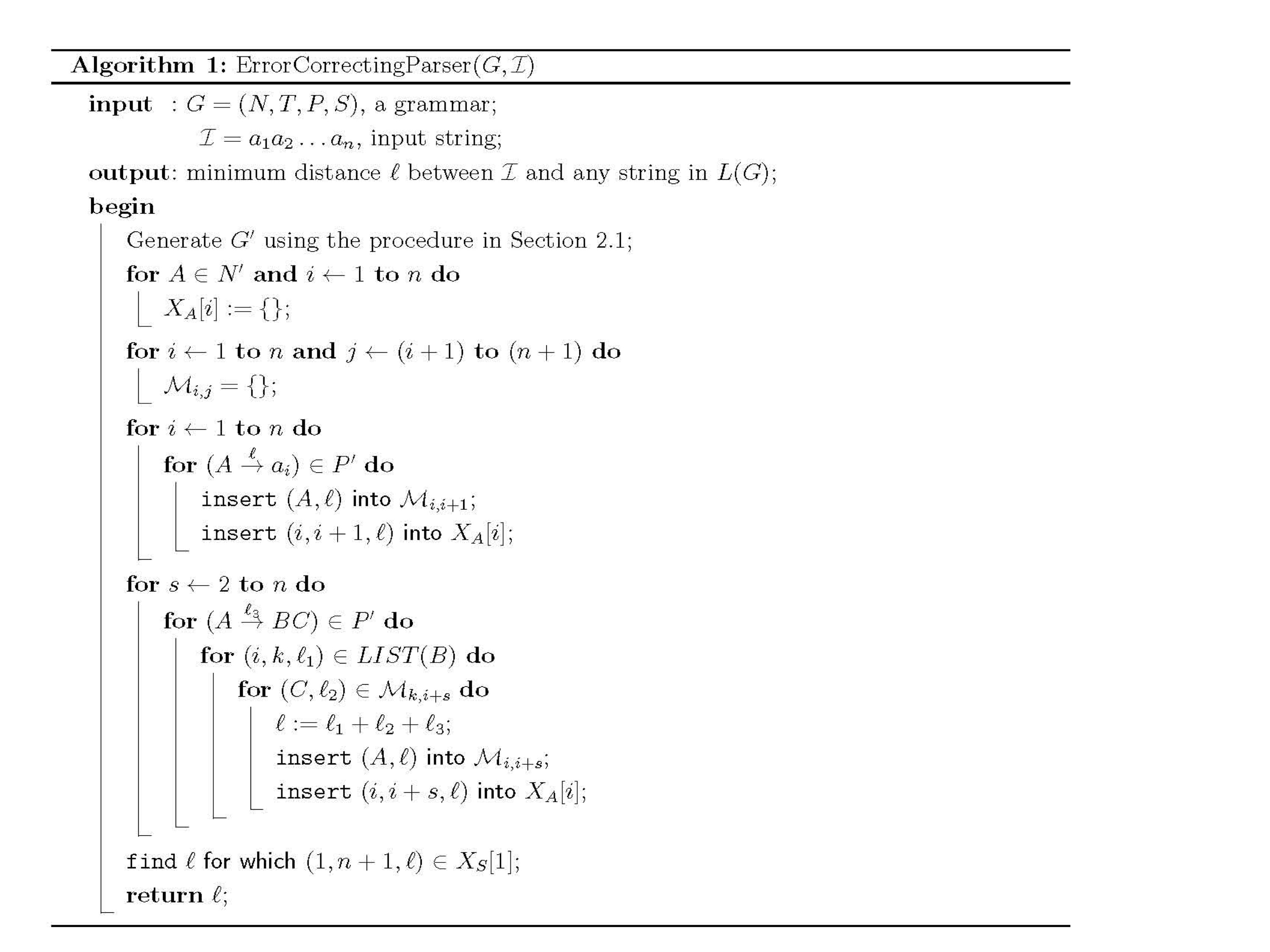
The algorithm is a modified version of an algorithm given in [10]. This algorithm in turn is a slightly different version of the CYK algorithm. Let be the grammar generated using the procedure given in Section 2.1. The basic idea behind the algorithm is the following: The algorithm has stages. In any given stage we scan through each production in and grow larger and larger parse trees. At any given time in the algorithm, each nonterminal has a list of tuples of the form . If is any nonterminal, will have tuples such that and there is no such that . If is a production in , then in any stage we process this production as follows: We scan through elements in and look for matches in . For instance, if is in (for some integer ), we check if is in , for some and . If so, we insert into . If for any has many tuples of the form we keep only one among these. Specifically, if are in , we keep only where .
We maintain the following data structures: (1) for each nonterminal , an array (call it ) of lists indexed 1 through , where is the list of all tuples from whose first item is ; and (2) an upper triangular matrix whose th entry will be those nonterminals that derive with the corresponding (minimum) error counts (for and ). There can be entries in , and for each entry in this list, we need to search for at most items in .
By induction, we can show that at the end of stage ), the algorithm would have computed all the nonterminals that span any input segment of length or less, together with the minimum error counts. (We say a nonterminal spans the input segment if it derives ; the nonterminal is said to have a ”span-length” of .)
A straight forward implementation of the above idea takes time. However, we can reduce the run time of each stage to as follows: In stage , while processing the production , work only with tuples from and whose combination will derive an input segment of length exactly . For example, if is a tuple in , the only tuple in we should look for is (for any integer ). We can look for such a tuple in time using the matrix . With this modification, each stage of the above algorithm will only take time and hence the total run time of the algorithm is . The pseudocode is given in algorithm 1.
Theorem 2.1
When the above algorithm completes, for any nonterminal , has a tuple if and only if and there is no such that .
Proof: The proof is by induction on the stage number .
Base Case: is when , i.e., , for . Note that all the nonterminals other than and are nullable. As a result, will have a production of the kind for every nonterminal and every terminal , for some integer . By the way we compute for each nonterminal and eliminate unit productions, it is clear that is the smallest integer for which .
Induction Step: Assume that the hypothesis is true for span lengths up to . We can prove it for a span length of . Let be any production in . Let be a tuple in and be a tuple in with . Then this means that , where . We add the tuple to . Also, the induction hypothesis implies that and there is no for which . Likewise, is the smallest integer for which . We consider all such productions in that will contribute tuples of the kind to and from these only keep where is the least such integer.
3 Less than Cubic Time Parser
In this section we present an error correcting parser that runs in time where is the length of the input string and is the time needed to compute the tropical product of two matrices. There are two main ingredients in this parser, namely, the procedure given in Section 2.1 for converting the given grammar into a covering grammar and Valiant’s reduction given in [13] (and summarized in Section 1.2.2).
As pointed out in Section 1.2.2, Valiant has presented an efficient algorithm for computing the transitive closure of an upper triangular matrix. The transitive closure is with respect to matrix multiplication defined in a special way. Each element in a matrix will be a set of items. In standard matrix multiplication we have two operators, namely, multiplication and addition. In the case of special matrix multiplication, these operations are replaced by and (called union). Valiant’s algorithm works as long as these operations satisfy the following properties: The outer operation (i.e., union) is commutative and associative, the inner operation distributes over union, is a zero with respect to and an identity with respect to union.
Valiant has shown that transitive closure under the above definition of matrix multiplication can be computed in time, where is the time needed for multiplying two matrices with the above special definition of matrix product.
In the context of error correcting parser we define the two operations as follows. Let be the input string. Matrix elements are sets of pairs of the kind where is a nonterminal and is an integer. We initialize an upper triangular matrix as:
| (1) |
If and are sets of pairs of the kind then is defined with the procedure in algorithm 2.
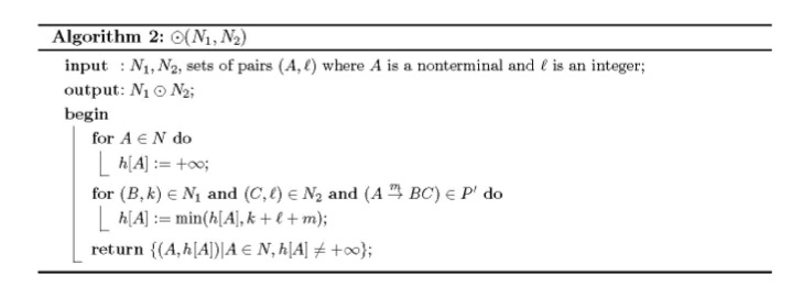
If and are sets of pairs of the kind , the union operation is defined as:
It is easy to see that the union operation is commutative and associative since if there are multiple pairs for the same nonterminal with different error counts, the union operation has the effect of keeping only one pair for each nonterminal with the least error count.
We can also verify that distributes over union. Let , and be any three sets of pairs of the type . Let , and . If , and , then . Also, and . Thus, .
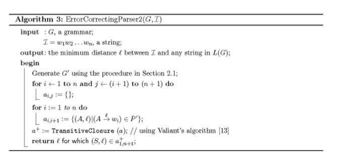
Put together, we get the following algorithm. Given a grammar and an input string , generate the grammar using the procedure in Section 2.1. Construct the matrix described in Equation 1. Compute the transitive closure of using Valiant’s algorithm [13]. will occur in for some integer . In this case, the minimum distance between and any string in is . The pseudocode is given in algorithm 3.
Note that, by definition,
where and
It is easy to see that , where is a nonterminal and is an integer in the range , will be in if and only if such that and there is no such that . Also, if .
As a result, will be in if and only if and there is no such that .
We get the following
Theorem 3.1
Error correcting parsing can be done in time where is the time needed to multiply two matrices under the new definition of matrix product.
It remains to be shown that where is the time needed to compute the tropical product of two matrices.
Let and be two matrices where the matrix elements are sets of pairs of the kind where is a nonterminal and is an integer. Let be the product of interest under the special definition of matrix product.
For each nonterminal in , we define a matrix and for each nonterminal in , we define a matrix . if , for . Likewise, if , for . The pseudocode of this operation is given in algorithm 4. Compute the tropical product of and for every nonterminal and every nonterminal .
For every production in do the following: for every , if then add to , keeping only the smallest distance if is already present in . The pseudocode is given in algorithm 5.
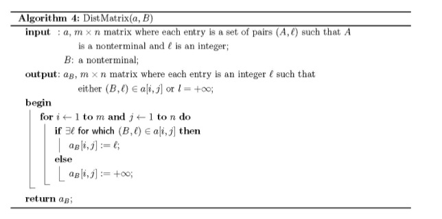
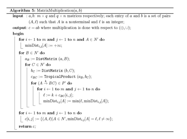
Clearly, the time spent in computing (under the new special definition of matrix product) is assuming that the size of the grammar is .
Put together we get the following theorem.
Theorem 3.2
Error correcting parsing can be done in time where is the time needed to compute the tropical product of two matrices.
Using the currently best known algorithm for tropical products [2], we get the following theorem.
Theorem 3.3
Error correcting parsing can be done in time.
Furthermore, consider the case of error correcting parsing where we know a priori that there exists a string in such that the distance between and is upper bounded by . We can solve this version of the language edit distance problem using the tropical matrix product algorithm of Zwick [15]. This algorithm multiplies two integer matrices in time if the matrix elements are in the range [15]. Here is the time taken to multiply two real matrices. Recall that when we reduce the matrix multiplication under and to tropical matrix multiplication, we have to compute the tropical product of and for every nonterminal and every nonterminal . Elements of and are integers in the range . Note that even if all the elements of are , some of the elements of and could be larger than . Before using the algorithm of [15] we have to ensure that all the elements of and are less than (where is some function of ). This can be done as follows. Before invoking the algorithm of [15], we replace every element of and by if the element is . is ’infinity’ as far as this multiplication is concerned. By doing this replacement, we are not affecting the final result of the algorithm and at the same time, we are making sure that the elements of and are .
As a result, we get the following theorem.
Theorem 3.4
Error correcting parsing can be done in time where is an upper bound on the edit distance between the input string and some string in , being the input CFG. is the time it takes to multiply two matrices.
As a corollary to the above theorem we can also get the following theorem.
Theorem 3.5
There exists an -approximation algorithm for the language edit distance problem that has a run time of , where is the time taken to multiply two matrices.
Proof: Here again, we replace every element of and by if the element is . In this case the elements of will be . We replace any element in that is larger than with . In general whenever we generate or operate on a matrix, we will ensure that the elements are . If for some , then the final answer output will be exact. If , then the algorithm will always output . Thus the theorem follows.
4 Retrieving
In all the algorithms presented above, we have focused on computing the minimum edit distance between the input string and any string in . In this section we address the problem of finding . We show that can be found in time, where . Let such that there is no such that . Let .
Realize that in the algorithms given in Section 2.2 and Section 3 we compute, for every and (with ), all the nonterminals such that spans and we also determine the least such that . In this case, there will be an entry for in the matrix . Specifically, will be in . We can utilize this information to identify an such that the edit distance between and is equal to . Note that we can deduce if we know the sequence of productions used to derive . The pseudocode is given in algorithm 6. We will invoke the algorithm as .
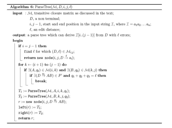
Algorithm 6 finds the first production in time. Having found the first production, we can proceed in a similar manner to find the other productions needed to derive . In the second stage we have to find a production that can be used to derive from and another production that can be used to derive from . Note that the span length of plus the span length of is and hence both the productions can be found in a total of time.
We can think of a tree where is the root and has two children and . If is the first production that can be used to derive from and is the first production that can be used to derive from , then will have two children and and will have two children and .
The rest of the tree is constructed in the same way. Clearly, the total span length of all the nonterminals in any level of the tree is and hence the time spent at each level is . Also, there can be at most levels. As a result, we get the following theorem.
Theorem 4.1
We can identify in time.
5 Conclusions
In this paper we have presented an error correcting parser for general context free languages. This algorithm takes less than cubic time, improving the 1972 algorithm of Aho and Peterson that has remained the best until now. We have also shown that if is an upper bound on the edit distance between the input string and some string of , then we can solve the parsing problem in time, where is the time it takes to multiply two matrices. As a corollary, we have presented an -approximation algorithm for the general context free language edit distance problem that runs in time .
Acknowledgements
This work has been supported in part by the following grant: NIH R01LM010101. The first author thanks Barna Saha for the introduction of this problem and Alex Russell for providing pointers to tropical matrix multiplication.
References
- [1] A.V. Aho and T.G. Peterson, A minimum distance error-correcting parser for context-free languages, SIAM Journal on Computing 1(4), 1972, 305-312.
- [2] T.M. Chan, More algorithms for all-pairs shortest paths in weighted graphs, SIAM Journal on Computing 39(5), 2010, 2075-2089.
- [3] J. Cocke and J.T. Schwartz, Programming languages and their compilers: Preliminary notes, Technical report, Courant Institute of Mathematical Sciences, New York University, 1970.
- [4] J. Earley, An efficient context-free parsing algorithm, Communications of the ACM 13, 1970, 94-102.
- [5] J.E. Hopcroft, R. Motwani, and J.D. Ullman, Introduction to Automata Theory, Languages, and Computation, Third Edition, Prentice Hall, July 9, 2006.
- [6] J. Kasami, An efficient recognition and syntax analysis algorithm for context-free languages, Report of Univ. of Hawaii, 1965.
- [7] F. Korn, B. Saha, D. Srivastava, and S. Ying, On repairing structural problems in semi-structured data, Proc. VLDB, 2013.
- [8] L. Lee, Fast context-free grammar parsing requires fast boolean matrix multiplication, Journal of the ACM 49(1), January 2002.
- [9] G. Myers, Approximately matching context-free languages, Information Processing Letters, 54, 1995.
- [10] S. Rajasekaran, Tree-adjoining language parsing in time, SIAM Journal on Computing, 25(4), 1996, 862-873.
- [11] S. Rajasekaran, S. Al Seesi, and R.A. Ammar, Improved algorithms for parsing ESLTAGs: a grammatical model suitable for RNA pseudoknots, IEEE/ACM Transactions on Computational Biology and Bioinformatics (TCBB), 7(4), 2010, pp. 619-627.
- [12] B. Saha, Efficiently computing edit distance to Dyck language, manuscript, November 2013.
- [13] L.G. Valiant, General context-free recognition in less than cubic time, Journal of Computer and System Sciences 10, 1975, 308-315.
- [14] D.H. Younger, Recognition and parsing of context-free languages in time , Information and Control 10, 1967, 189-208.
- [15] U. Zwick, All pairs shortest paths in weighted directed graphs-exact and almost exact algorithms, Foundations of Computer Science, 1998. Proceedings. 39th Annual Symposium on, IEEE, 1998.