跳到论文正文
W Papers独立论文阅读器 arXiv:1406.3339 论文正文 计算阅读时间 · 0%
引用这篇论文根据当前论文元数据生成,正式投稿前建议核对。


License: arXiv.org perpetual non-exclusive license
arXiv:1406.3339v3 [cs.AI] 10 Jul 2014

Algorithms for CVaR Optimization in MDPsThanks: Mohammad Ghavamzadeh is at Adobe Research, on leave of absence from INRIA Lille - Team SequeL.

Yinlam Chow Affiliation: Institute of Computational & Mathematical Engineering, Stanford University Affiliation: Mohammad Ghavamzadeh Affiliation: INRIA Lille - Team SequeL & Adobe Research
Abstract

In many sequential decision-making problems we may want to manage risk by minimizing some measure of variability in costs in addition to minimizing a standard criterion. Conditional value-at-risk (CVaR) is a relatively new risk measure that addresses some of the shortcomings of the well-known variance-related risk measures, and because of its computational efficiencies has gained popularity in finance and operations research. In this paper, we consider the mean-CVaR optimization problem in MDPs. We first derive a formula for computing the gradient of this risk-sensitive objective function. We then devise policy gradient and actor-critic algorithms that each uses a specific method to estimate this gradient and updates the policy parameters in the descent direction. We establish the convergence of our algorithms to locally risk-sensitive optimal policies. Finally, we demonstrate the usefulness of our algorithms in an optimal stopping problem.

1 Introduction

A standard optimization criterion for an infinite horizon Markov decision process (MDP) is the expected sum of (discounted) costs (i.e., finding a policy that minimizes the value function of the initial state of the system). However in many applications, we may prefer to minimize some measure of risk in addition to this standard optimization criterion. In such cases, we would like to use a criterion that incorporates a penalty for the variability (due to the stochastic nature of the system) induced by a given policy. In risk-sensitive MDPs [18], the objective is to minimize a risk-sensitive criterion such as the expected exponential utility [18], a variance-related measure [32, 16], or the percentile performance [17]. The issue of how to construct such criteria in a manner that will be both conceptually meaningful and mathematically tractable is still an open question.

Although most losses (returns) are not normally distributed, the typical Markiowitz mean-variance optimization [22], that relies on the first two moments of the loss (return) distribution, has dominated the risk management for over 5050 years. Numerous alternatives to mean-variance optimization have emerged in the literature, but there is no clear leader amongst these alternative risk-sensitive objective functions. Value-at-risk (VaR) and conditional value-at-risk (CVaR) are two promising such alternatives that quantify the losses that might be encountered in the tail of the loss distribution, and thus, have received high status in risk management. For (continuous) loss distributions, while VaR measures risk as the maximum loss that might be incurred w.r.t. a given confidence level α\alpha, CVaR measures it as the expected loss given that the loss is greater or equal to VaRα. Although VaR is a popular risk measure, CVaR’s computational advantages over VaR has boosted the development of CVaR optimization techniques. We provide the exact definitions of these two risk measures and briefly discuss some of the VaR’s shortcomings in Section 2. CVaR minimization was first developed by Rockafellar and Uryasev [29] and its numerical effectiveness was demonstrated in portfolio optimization and option hedging problems. Their work was then extended to objective functions consist of different combinations of the expected loss and the CVaR, such as the minimization of the expected loss subject to a constraint on CVaR. This is the objective function that we study in this paper, although we believe that our proposed algorithms can be easily extended to several other CVaR-related objective functions. Boda and Filar [10] and Bäuerle and Ott [25, 4] extended the results of [29] to MDPs (sequential decision-making). While the former proposed to use dynamic programming (DP) to optimize CVaR, an approach that is limited to small problems, the latter showed that in both finite and infinite horizon MDPs, there exists a deterministic history-dependent optimal policy for CVaR optimization (see Section 3 for more details).

Most of the work in risk-sensitive sequential decision-making has been in the context of MDPs (when the model is known) and much less work has been done within the reinforcement learning (RL) framework. In risk-sensitive RL, we can mention the work by Borkar [11, 12] who considered the expected exponential utility and those by Tamar et al. [34] and Prashanth and Ghavamzadeh [21] on several variance-related risk measures. CVaR optimization in RL is a rather novel subject. Morimura et al. [24] estimate the return distribution while exploring using a CVaR-based risk-sensitive policy. Their algorithm does not scale to large problems. Petrik and Subramanian [27] propose a method based on stochastic dual DP to optimize CVaR in large-scale MDPs. However, their method is limited to linearly controllable problems. Borkar and Jain [15] consider a finite-horizon MDP with CVaR constraint and sketch a stochastic approximation algorithm to solve it. Finally, Tamar et al. [35] have recently proposed a policy gradient algorithm for CVaR optimization.

In this paper, we develop policy gradient (PG) and actor-critic (AC) algorithms for mean-CVaR optimization in MDPs. We first derive a formula for computing the gradient of this risk-sensitive objective function. We then propose several methods to estimate this gradient both incrementally and using system trajectories (update at each time-step vs. update after observing one or more trajectories). We then use these gradient estimations to devise PG and AC algorithms that update the policy parameters in the descent direction. Using the ordinary differential equations (ODE) approach, we establish the asymptotic convergence of our algorithms to locally risk-sensitive optimal policies. Finally, we demonstrate the usefulness of our algorithms in an optimal stopping problem. In comparison to [35], while they develop a PG algorithm for CVaR optimization in stochastic shortest path problems that only considers continuous loss distributions, uses a biased estimator for VaR, is not incremental, and has no convergence proof, here we study mean-CVaR optimization, consider both discrete and continuous loss distributions, devise both PG and (several) AC algorithms (trajectory-based and incremental – plus AC helps in reducing the variance of PG algorithms), and establish convergence proof for our algorithms.

2 Preliminaries

We consider problems in which the agent’s interaction with the environment is modeled as a MDP. A MDP is a tuple ℳ=(𝒳,𝒜,C,P,P0)\mathcal{M}=(\mathcal{X},\mathcal{A},C,P,P_{0}), where 𝒳={1,…,n}\mathcal{X}=\{1,\ldots,n\} and 𝒜={1,…,m}\mathcal{A}=\{1,\ldots,m\} are the state and action spaces; C⁡(x,a)∈[−Cmax,Cmax]C(x,a)\in[-C_{\max},C_{\max}] is the bounded cost random variable whose expectation is denoted by c⁡(x,a)=𝔼⁡[C⁡(x,a)]c(x,a)=\mathbb{E}\big[C(x,a)\big]; P(⋅|x,a)P(\cdot|x,a) is the transition probability distribution; and P0​(⋅)P_{0}(\cdot) is the initial state distribution. For simplicity, we assume that the system has a single initial state x0x^{0}, i.e., P0(x)=𝟏{x=x0}P_{0}(x)=\mathbf{1}\{x=x^{0}\}. All the results of the paper can be easily extended to the case that the system has more than one initial state. We also need to specify the rule according to which the agent selects actions at each state. A stationary policy μ(⋅|x)\mu(\cdot|x) is a probability distribution over actions, conditioned on the current state. In policy gradient and actor-critic methods, we define a class of parameterized stochastic policies {μ(⋅|x;θ),x∈𝒳,θ∈Θ⊆Rκ1}\big\{\mu(\cdot|x;\theta),x\in\mathcal{X},\theta\in\Theta\subseteq R^{\kappa_{1}}\big\}, estimate the gradient of a performance measure w.r.t. the policy parameters θ\theta from the observed system trajectories, and then improve the policy by adjusting its parameters in the direction of the gradient. Since in this setting a policy μ\mu is represented by its κ1\kappa_{1}-dimensional parameter vector θ\theta, policy dependent functions can be written as a function of θ\theta in place of μ\mu. So, we use μ\mu and θ\theta interchangeably in the paper. We denote by dγμ​(x|x0)=(1−γ)​∑k=0∞γk​ℙ​(xk=x|x0=x0;μ)d_{\gamma}^{\mu}(x|x^{0})=(1-\gamma)\sum_{k=0}^{\infty}\gamma^{k}\mathbb{P}(x_{k}=x|x_{0}=x^{0};\mu) and πγμ​(x,a|x0)=dγμ​(x|x0)​μ​(a|x)\pi_{\gamma}^{\mu}(x,a|x^{0})=d_{\gamma}^{\mu}(x|x^{0})\mu(a|x) the γ\gamma-discounted visiting distribution of state xx and state-action pair (x,a)(x,a) under policy μ\mu, respectively.

Let ZZ be a bounded-mean random variable, i.e., 𝔼⁡[|Z|]<∞\mathbb{E}[|Z|]<\infty, with the cumulative distribution function F⁡(z)=ℙ⁡(Z≤z)F(z)=\mathbb{P}(Z\leq z) (e.g., one may think of ZZ as the loss of an investment strategy μ\mu). We define the value-at-risk at the confidence level α∈(0,1)\alpha\in(0,1) as VaR(Z)α=min{z∣F(z)≥α}{}_{\alpha}(Z)=\min\big\{z\mid F(z)\geq\alpha\big\}. Here the minimum is attained because FF is non-decreasing and right-continuous in zz. When FF is continuous and strictly increasing, VaR(Z)α{}_{\alpha}(Z) is the unique zz satisfying F⁡(z)=αF(z)=\alpha, otherwise, the VaR equation can have no solution or a whole range of solutions. Although VaR is a popular risk measure, it suffers from being unstable and difficult to work with numerically when ZZ is not normally distributed, which is often the case as loss distributions tend to exhibit fat tails or empirical discreteness. Moreover, VaR is not a coherent risk measure [2] and more importantly does not quantify the losses that might be suffered beyond its value at the α\alpha-tail of the distribution [28]. An alternative measure that addresses most of the VaR’s shortcomings is conditional value-at-risk, CVAR(Z)α{}_{\alpha}(Z), which is the mean of the α\alpha-tail distribution of ZZ. If there is no probability atom at VaR(Z)α{}_{\alpha}(Z), CVaR(Z)α{}_{\alpha}(Z) has a unique value that is defined as CVaR(Z)α=𝔼[Z∣Z≥VaRα(Z)]{}_{\alpha}(Z)=\mathbb{E}\big[Z\mid Z\geq\text{VaR}_{\alpha}(Z)\big]. Rockafellar and Uryasev [29] showed that

CVaRα​(Z)=minν∈⁡Hα​(Z,ν)=△minν∈⁡{ν+11−α​𝔼​[(Z−ν)+]}.\text{CVaR}_{\alpha}(Z)=\min_{\nu\in\real}H_{\alpha}(Z,\nu)\stackrel{{\scriptstyle\triangle}}{{=}}\min_{\nu\in\real}\Big\{\nu+\frac{1}{1-\alpha}\mathbb{E}\big[(Z-\nu)^{+}\big]\Big\}. (1)

Note that as a function of ν\nu, Hα​(⋅,ν)H_{\alpha}(\cdot,\nu) is finite and convex (hence continuous).

3 CVaR Optimization in MDPs

For a policy μ\mu, we define the loss of a state xx (state-action pair (x,a)(x,a)) as the sum of (discounted) costs encountered by the agent when it starts at state xx (state-action pair (x,a)(x,a)) and then follows policy μ\mu, i.e., Dθ​(x)=∑k=0∞γk​C​(xk,ak)|x0=x,μ\;D^{\theta}(x)=\sum_{k=0}^{\infty}\gamma^{k}C(x_{k},a_{k})\mid x_{0}=x,\;\mu\; and Dθ(x,a)=∑k=0∞γkC(xk,ak)∣x0=x,a0=a,μ\;D^{\theta}(x,a)=\sum_{k=0}^{\infty}\gamma^{k}C(x_{k},a_{k})\mid x_{0}=x,\;a_{0}=a,\;\mu. The expected value of these two random variables are the value and action-value functions of policy μ\mu, i.e., Vθ​(x)=𝔼⁡[Dθ​(x)]V^{\theta}(x)=\mathbb{E}\big[D^{\theta}(x)\big] and Qθ​(x,a)=𝔼⁡[Dθ​(x,a)]Q^{\theta}(x,a)=\mathbb{E}\big[D^{\theta}(x,a)\big]. The goal in the standard discounted formulation is to find an optimal policy θ∗=argminθVθ​(x0)\theta^{*}=\operatornamewithlimits{argmin}_{\theta}V^{\theta}(x^{0}).

For CVaR optimization in MDPs, we consider the following optimization problem: For a given confidence level α∈(0,1)\alpha\in(0,1) and loss tolerance β∈\beta\in\real,

minθ⁡Vθ​(x0)subject toCVaRα​(Dθ​(x0))≤β.\min_{\theta}V^{\theta}(x^{0})\hskip 9.24994pt\hskip 9.24994pt\text{subject to}\hskip 9.24994pt\hskip 9.24994pt\text{CVaR}_{\alpha}\big(D^{\theta}(x^{0})\big)\leq\beta. (2)

By Theorem 16 in [28], the optimization problem (2) is equivalent to (HαH_{\alpha} is defined by (1))

minθ,ν⁡Vθ​(x0)subject toHα​(Dθ​(x0),ν)≤β.\min_{\theta,\nu}V^{\theta}(x^{0})\hskip 9.24994pt\hskip 9.24994pt\text{subject to}\hskip 9.24994pt\hskip 9.24994ptH_{\alpha}\big(D^{\theta}(x^{0}),\nu\big)\leq\beta. (3)

To solve (3), we employ the Lagrangian relaxation procedure [5] to convert it to the following unconstrained problem:

maxλ⁡minθ,ν⁡(L⁡(θ,ν,λ)=△Vθ​(x0)+λ⁡(Hα​(Dθ​(x0),ν)−β)),\max_{\lambda}\min_{\theta,\nu}\bigg(L(\theta,\nu,\lambda)\stackrel{{\scriptstyle\triangle}}{{=}}V^{\theta}(x^{0})+\lambda\Big(H_{\alpha}\big(D^{\theta}(x^{0}),\nu\big)-\beta\Big)\bigg), (4)

where λ\lambda is the Lagrange multiplier. The goal here is to find the saddle point of L⁡(θ,ν,λ)L(\theta,\nu,\lambda), i.e., a point (θ∗,ν∗,λ∗)(\theta^{*},\nu^{*},\lambda^{*}) that satisfies L⁡(θ,ν,λ∗)≥L⁡(θ∗,ν∗,λ∗)≥L⁡(θ∗,ν∗,λ),∀θ,ν,∀λ>0L(\theta,\nu,\lambda^{*})\geq L(\theta^{*},\nu^{*},\lambda^{*})\geq L(\theta^{*},\nu^{*},\lambda),\forall\theta,\nu,\forall\lambda>0. This is achieved by descending in (θ,ν)(\theta,\nu) and ascending in λ\lambda using the gradients of L⁡(θ,ν,λ)L(\theta,\nu,\lambda) w.r.t. θ\theta, ν\nu, and λ\lambda, i.e.,11 1 The notation ∋\ni in (6) means that the right-most term is a member of the sub-gradient set ∂νL⁡(θ,ν,λ)\partial_{\nu}L(\theta,\nu,\lambda).

∇θL​(θ,ν,λ)\displaystyle\nabla_{\theta}L(\theta,\nu,\lambda) =∇θVθ​(x0)+λ(1−α)​∇θ𝔼​[(Dθ​(x0)−ν)+],\displaystyle=\nabla_{\theta}V^{\theta}(x^{0})+\frac{\lambda}{(1-\alpha)}\nabla_{\theta}\mathbb{E}\Big[\big(D^{\theta}(x^{0})-\nu\big)^{+}\Big], (5)
∂νL⁡(θ,ν,λ)\displaystyle\partial_{\nu}L(\theta,\nu,\lambda) =λ⁡(1+1(1−α)​∂ν𝔼⁡[(Dθ​(x0)−ν)+])∋λ⁡(1−1(1−α)​ℙ​(Dθ​(x0)≥ν)),\displaystyle=\lambda\bigg(1+\frac{1}{(1-\alpha)}\partial_{\nu}\mathbb{E}\Big[\big(D^{\theta}(x^{0})-\nu\big)^{+}\Big]\bigg)\ni\lambda\bigg(1-\frac{1}{(1-\alpha)}\mathbb{P}\big(D^{\theta}(x^{0})\geq\nu\big)\bigg), (6)
∇λL​(θ,ν,λ)\displaystyle\nabla_{\lambda}L(\theta,\nu,\lambda) =ν+1(1−α)​𝔼​[(Dθ​(x0)−ν)+]−β.\displaystyle=\nu+\frac{1}{(1-\alpha)}\mathbb{E}\Big[\big(D^{\theta}(x^{0})-\nu\big)^{+}\Big]-\beta. (7)

We assume that there exists a policy μ(⋅|⋅;θ)\mu(\cdot|\cdot;\theta) such that CVaR(Dθ(x0))α≤β{}_{\alpha}\big(D^{\theta}(x^{0})\big)\leq\beta (feasibility assumption). As discussed in Section 1, Bäuerle and Ott [25, 4] showed that there exists a deterministic history-dependent optimal policy for CVaR optimization. The important point is that this policy does not depend on the complete history, but only on the current time step kk, current state of the system xkx_{k}, and accumulated discounted cost ∑i=0kγi​c​(xi,ai)\sum_{i=0}^{k}\gamma^{i}c(x_{i},a_{i}).

In the following, we present a policy gradient (PG) algorithm (Sec. 4) and several actor-critic (AC) algorithms (Sec. 5.5) to optimize (4). While the PG algorithm updates its parameters after observing several trajectories, the AC algorithms are incremental and update their parameters at each time-step.

4 A Trajectory-based Policy Gradient Algorithm

In this section, we present a policy gradient algorithm to solve the optimization problem (4). The unit of observation in this algorithm is a system trajectory generated by following the current policy. At each iteration, the algorithm generates NN trajectories by following the current policy, use them to estimate the gradients in (5)-(7), and then use these estimates to update the parameters θ,ν,λ\theta,\nu,\lambda.

Let ξ={x0,a0,c0,x1,a1,c1,…,xT−1,aT−1,cT−1,xT}\xi=\{x_{0},a_{0},c_{0},x_{1},a_{1},c_{1},\ldots,x_{T-1},a_{T-1},c_{T-1},x_{T}\} be a trajectory generated by following the policy θ\theta, where x0=x0x_{0}=x^{0} and xTx_{T} is usually a terminal state of the system. After xkx_{k} visits the terminal state, it enters a recurring sink state xRx_{R} at the next time step, incurring zero cost, i.e., C⁡(xR,a)=0C(x_{R},a)=0, ∀a∈𝒜\forall a\in\mathcal{A}. Time index TT is referred as the stopping time of the MDP. Since the transition is stochastic, TT is a non-deterministic quantity. Here we assume that the policy μ\mu is proper, i.e., ∑k=0∞ℙ⁡(xk=x|x0=x0,μ)<∞\sum_{k=0}^{\infty}\mathbb{P}(x_{k}=x|x_{0}=x^{0},\mu)<\infty for every x∉{xS,xT}x\not\in\{x_{S},x_{T}\}. This further means that with probability 11, the MDP exits the transient states and hits xTx_{T} (and stays in xSx_{S}) in finite time TT. For simplicity, we assume that the agent incurs zero cost in the terminal state. Analogous results for the general case with a non-zero terminal cost can be derived using identical arguments. The loss and probability of ξ\xi are defined as D⁡(ξ)=∑k=0T−1γk​c​(xk,ak)D(\xi)=\sum_{k=0}^{T-1}\gamma^{k}c(x_{k},a_{k}) and ℙθ​(ξ)=P0​(x0)​∏k=0T−1μ⁡(ak|xk;θ)​P​(xk+1|xk,ak)\mathbb{P}_{\theta}(\xi)=P_{0}(x_{0})\prod_{k=0}^{T-1}\mu(a_{k}|x_{k};\theta)P(x_{k+1}|x_{k},a_{k}), respectively. It can be easily shown that ∇θ​log​ℙθ​(ξ)=∑k=0T−1∇θ​log​μ​(ak|xk;θ)\nabla_{\theta}\log\mathbb{P}_{\theta}(\xi)=\sum_{k=0}^{T-1}\nabla_{\theta}\log\mu(a_{k}|x_{k};\theta).

Algorithm 1 contains the pseudo-code of our proposed policy gradient algorithm. What appears inside the parentheses on the right-hand-side of the update equations are the estimates of the gradients of L⁡(θ,ν,λ)L(\theta,\nu,\lambda) w.r.t. θ,ν,λ\theta,\nu,\lambda (estimates of (5)-(7)) (see Appendix A.2). ΓΘ\Gamma_{\Theta} is an operator that projects a vector θ∈κ1\theta\in\real^{\kappa_{1}} to the closest point in a compact and convex set Θ⊂κ1\Theta\subset\real^{\kappa_{1}}, and ΓN\Gamma_{N} and ΓΛ\Gamma_{\Lambda} are projection operators to [−Cmax1−γ,Cmax1−γ][-\frac{C_{\max}}{1-\gamma},\frac{C_{\max}}{1-\gamma}] and [0,λmax][0,\lambda_{\max}], respectively. These projection operators are necessary to ensure the convergence of the algorithm. The step-size schedules satisfy the standard conditions for stochastic approximation algorithms, and ensures that the VaR parameter ν\nu update is on the fastest time-scale {ζ3​(i)}\big\{\zeta_{3}(i)\big\}, the policy parameter θ\theta update is on the intermediate time-scale {ζ2​(i)}\big\{\zeta_{2}(i)\big\}, and the Lagrange multiplier λ\lambda update is on the slowest time-scale {ζ1​(i)}\big\{\zeta_{1}(i)\big\} (see Appendix A.1 for the conditions on the step-size schedules). This results in a three time-scale stochastic approximation algorithm. We prove that our policy gradient algorithm converges to a (local) saddle point of the risk-sensitive objective function L⁡(θ,ν,λ)L(\theta,\nu,\lambda) (see Appendix A.3).

 Input: parameterized policy μ(⋅|⋅;θ)\mu(\cdot|\cdot;\theta), confidence level α\alpha, loss tolerance β\beta and Lagrangian threshold λmax\lambda_{\max}
 Initialization: policy parameter θ=θ0\theta=\theta_{0}, VaR parameter ν=ν0\nu=\nu_{0}, and the Lagrangian parameter λ=λ0\lambda=\lambda_{0}
 while 1 do
  for i=0,1,2,…i=0,1,2,\ldots do
   for j=1,2,…j=1,2,\ldots do
     Generate NN trajectories {ξj,i}j=1N\{\xi_{j,i}\}_{j=1}^{N} by starting at x0=x0x_{0}=x^{0} and following the current policy θi\theta_{i}.
   end for
ν\nu Update:    νi+1=ΓN[νi−ζ3(i)(λi−λi(1−α)​N∑j=1N𝟏{D(ξj,i)≥νi})]\displaystyle\nu_{i+1}=\Gamma_{N}\bigg[\nu_{i}-\zeta_{3}(i)\bigg(\lambda_{i}-\frac{\lambda_{i}}{(1-\alpha)N}\sum_{j=1}^{N}\mathbf{1}\big\{D(\xi_{j,i})\geq\nu_{i}\big\}\bigg)\bigg]
θ\theta Update:    θi+1=ΓΘ[θi−ζ2(i)(1N∑j=1N∇θlogℙθ(ξj,i)|θ=θiD(ξj,i)\displaystyle\theta_{i+1}=\Gamma_{\Theta}\bigg[\theta_{i}-\zeta_{2}(i)\bigg(\frac{1}{N}\sum_{j=1}^{N}\nabla_{\theta}\log\mathbb{P}_{\theta}(\xi_{j,i})|_{\theta=\theta_{i}}D(\xi_{j,i})
+λi(1−α)​N∑j=1N∇θlogℙθ(ξj,i)|θ=θi(D(ξj,i)−νi)𝟏{D(ξj,i)≥νi})]\displaystyle\hskip 52.39618pt+\frac{\lambda_{i}}{(1-\alpha)N}\sum_{j=1}^{N}\nabla_{\theta}\log\mathbb{P}_{\theta}(\xi_{j,i})|_{\theta=\theta_{i}}\big(D(\xi_{j,i})-\nu_{i}\big)\mathbf{1}\big\{D(\xi_{j,i})\geq\nu_{i}\big\}\bigg)\bigg]
λ\lambda Update:    λi+1=ΓΛ[λi+ζ1(i)(νi−β+1(1−α)​N∑j=1N(D(ξj,i)−νi)𝟏{D(ξj,i)≥νi})]\displaystyle\lambda_{i+1}=\Gamma_{\Lambda}\bigg[\lambda_{i}+\zeta_{1}(i)\bigg(\nu_{i}-\beta+\frac{1}{(1-\alpha)N}\sum_{j=1}^{N}\big(D(\xi_{j,i})-\nu_{i}\big)\mathbf{1}\big\{D(\xi_{j,i})\geq\nu_{i}\big\}\bigg)\bigg]
  end for
  if {λi}\{\lambda_{i}\} converges to λmax\lambda_{\max} then
   Set λmax←2​λmax\lambda_{\max}\leftarrow 2\lambda_{\max}.
  else
   return parameters ν,θ,λ\nu,\theta,\lambda and break
  end if
 end while
Algorithm 1 Trajectory-based Policy Gradient Algorithm for CVaR Optimization

5 Incremental Actor-Critic Algorithms

As mentioned in Section 4, the unit of observation in our policy gradient algorithm (Algorithm 1) is a system trajectory. This may result in high variance for the gradient estimates, especially when the length of the trajectories is long. To address this issue, in this section, we propose actor-critic algorithms that use linear approximation for some quantities in the gradient estimates and update the parameters incrementally (after each state-action transition). To develop our actor-critic algorithms, we should show how the gradients of (5)-(7) are estimated in an incremental fashion. We show this in the next four subsections, followed by a subsection that contains the algorithms.

5.1 Gradient w.r.t. the Policy Parameters θ\theta

The gradient of our objective function w.r.t. the policy parameters θ\theta in (5) may be rewritten as

∇θL​(θ,ν,λ)=∇θ(𝔼⁡[Dθ​(x0)]+λ(1−α)​𝔼​[(Dθ​(x0)−ν)+]).\nabla_{\theta}L(\theta,\nu,\lambda)=\nabla_{\theta}\left(\mathbb{E}\big[D^{\theta}(x^{0})\big]+\frac{\lambda}{(1-\alpha)}\mathbb{E}\Big[\big(D^{\theta}(x^{0})-\nu\big)^{+}\Big]\right). (8)

Given the original MDP ℳ=(𝒳,𝒜,C,P,P0)\mathcal{M}=(\mathcal{X},\mathcal{A},C,P,P_{0}) and the parameter λ\lambda, we define the augmented MDP ℳ¯=(𝒳¯,𝒜¯,C¯,P¯,P¯0)\bar{\mathcal{M}}=(\bar{\mathcal{X}},\bar{\mathcal{A}},\bar{C},\bar{P},\bar{P}_{0}) as 𝒳¯=𝒳×\bar{\mathcal{X}}=\mathcal{X}\times\real, 𝒜¯=𝒜\bar{\mathcal{A}}=\mathcal{A}, P¯0(x,s)=P0(x)𝟏{s=s0}\bar{P}_{0}(x,s)=P_{0}(x)\mathbf{1}\{s=s^{0}\}, and

C¯​(x,s,a)\displaystyle\bar{C}(x,s,a) ={λ​(−s)+/(1−α)if x=xTC⁡(x,a)otherwise,\displaystyle=\left\{\begin{array}[]{cc}\lambda(-s)^{+}/(1-\alpha)&\text{if $x=x_{T}$}\\ C(x,a)&\text{otherwise}\end{array}\right.\!\!, P¯(x′,s′|x,s,a)={P⁡(x′|x,a)if s′=(s−C⁡(x,a))/γ0otherwise\displaystyle\,\bar{P}(x^{\prime},s^{\prime}|x,s,a)=\left\{\begin{array}[]{ll}P(x^{\prime}|x,a)&\text{if $s^{\prime}=\big(s-C(x,a)\big)/\gamma$}\\ 0&\text{otherwise}\end{array}\right.

where xTx_{T} is any terminal state of the original MDP ℳ\mathcal{M} and sTs_{T} is the value of the ss part of the state when a policy θ\theta reaches a terminal state xTx_{T} after TT steps, i.e., sT=1γT​(s0−∑k=0T−1γk​C​(xk,ak))s_{T}=\frac{1}{\gamma^{T}}\big(s^{0}-\sum_{k=0}^{T-1}\gamma^{k}C(x_{k},a_{k})\big). We define a class of parameterized stochastic policies {μ(⋅|x,s;θ),(x,s)∈𝒳¯,θ∈Θ⊆Rκ1}\big\{\mu(\cdot|x,s;\theta),(x,s)\in\bar{\mathcal{X}},\theta\in\Theta\subseteq R^{\kappa_{1}}\big\} for this augmented MDP. Thus, the total (discounted) loss of this trajectory can be written as

∑k=0T−1γk​C​(xk,ak)+γT​C¯​(xT,sT,a)=Dθ​(x0)+λ(1−α)​(Dθ​(x0)−s0)+.\sum_{k=0}^{T-1}\gamma^{k}C(x_{k},a_{k})+\gamma^{T}\bar{C}(x_{T},s_{T},a)=D^{\theta}(x^{0})+\frac{\lambda}{(1-\alpha)}\big(D^{\theta}(x^{0})-s^{0}\big)^{+}. (9)

From (9), it is clear that the quantity in the parenthesis of (8) is the value function of the policy θ\theta at state (x0,s0=ν)(x^{0},s^{0}=\nu) in the augmented MDP ℳ¯\bar{\mathcal{M}}, i.e., Vθ​(x0,ν)V^{\theta}(x^{0},\nu). Thus, it is easy to show that (the proof of the second equality can be found in the literature, e.g., [26])

∇θL(θ,ν,λ)=∇θVθ(x0,ν)=11−γ∑x,s,aπγθ(x,s,a|x0,ν)∇logμ(a|x,s;θ)Qθ(x,s,a),\nabla_{\theta}L(\theta,\nu,\lambda)=\nabla_{\theta}V^{\theta}(x^{0},\nu)=\frac{1}{1-\gamma}\sum_{x,s,a}\pi_{\gamma}^{\theta}(x,s,a|x^{0},\nu)\;\nabla\log\mu(a|x,s;\theta)\;Q^{\theta}(x,s,a), (10)

where πγθ\pi_{\gamma}^{\theta} is the discounted visiting distribution (defined in Section 2) and QθQ^{\theta} is the action-value function of policy θ\theta in the augmented MDP ℳ¯\bar{\mathcal{M}}. We can show that 11−γ∇logμ(ak|xk,sk;θ)⋅δk\frac{1}{1-\gamma}\nabla\log\mu(a_{k}|x_{k},s_{k};\theta)\cdot\delta_{k} is an unbiased estimate of ∇θL​(θ,ν,λ)\nabla_{\theta}L(\theta,\nu,\lambda), where δk=C¯​(xk,sk,ak)+γ​V^​(xk+1,sk+1)−V^​(xk,sk)\delta_{k}=\bar{C}(x_{k},s_{k},a_{k})+\gamma\widehat{V}(x_{k+1},s_{k+1})-\widehat{V}(x_{k},s_{k}) is the temporal-difference (TD) error in ℳ¯\bar{\mathcal{M}}, and V^\widehat{V} is an unbiased estimator of VθV^{\theta} (see e.g. [8]). In our actor-critic algorithms, the critic uses linear approximation for the value function Vθ​(x,s)≈v⊤​ϕ​(x,s)=V~θ,v​(x,s)V^{\theta}(x,s)\approx v^{\top}\phi(x,s)=\widetilde{V}^{\theta,v}(x,s), where the feature vector ϕ⁡(⋅)\phi(\cdot) is from low-dimensional space κ2\real{}^{\kappa_{2}}.

5.2 Gradient w.r.t. the Lagrangian Parameter λ\lambda

We may rewrite the gradient of our objective function w.r.t. the Lagrangian parameters λ\lambda in (7) as

∇λL​(θ,ν,λ)=ν−β+∇λ(𝔼⁡[Dθ​(x0)]+λ(1−α)​𝔼​[(Dθ​(x0)−ν)+])=(a)ν−β+∇λVθ​(x0,ν).\nabla_{\lambda}L(\theta,\nu,\lambda)=\nu-\beta+\nabla_{\lambda}\left(\mathbb{E}\big[D^{\theta}(x^{0})\big]+\frac{\lambda}{(1-\alpha)}\mathbb{E}\Big[\big(D^{\theta}(x^{0})-\nu\big)^{+}\Big]\right)\stackrel{{\scriptstyle\text{(a)}}}{{=}}\nu-\beta+\nabla_{\lambda}V^{\theta}(x^{0},\nu). (11)

Similar to Section 5.1, (a) comes from the fact that the quantity in the parenthesis in (11) is Vθ​(x0,ν)V^{\theta}(x^{0},\nu), the value function of the policy θ\theta at state (x0,ν)(x^{0},\nu) in the augmented MDP ℳ¯\bar{\mathcal{M}}. Note that the dependence of Vθ​(x0,ν)V^{\theta}(x^{0},\nu) on λ\lambda comes from the definition of the cost function C¯\bar{C} in ℳ¯\bar{\mathcal{M}}. We now derive an expression for ∇λVθ​(x0,ν)\nabla_{\lambda}V^{\theta}(x^{0},\nu), which in turn will give us an expression for ∇λL​(θ,ν,λ)\nabla_{\lambda}L(\theta,\nu,\lambda).

Lemma 1

The gradient of Vθ​(x0,ν)V^{\theta}(x^{0},\nu) w.r.t. the Lagrangian parameter λ\lambda may be written as

∇λVθ(x0,ν)=11−γ∑x,s,aπγθ(x,s,a|x0,ν)1(1−α)𝟏{x=xT}(−s)+.\nabla_{\lambda}V^{\theta}(x^{0},\nu)=\frac{1}{1-\gamma}\sum_{x,s,a}\pi_{\gamma}^{\theta}(x,s,a|x^{0},\nu)\frac{1}{(1-\alpha)}\mathbf{1}\{x=x_{T}\}(-s)^{+}. (12)

Proof. See Appendix B.2. ■\blacksquare

From Lemma 1 and (11), it is easy to see that ν−β+1(1−γ)​(1−α)𝟏{x=xT}(−s)+\nu-\beta+\frac{1}{(1-\gamma)(1-\alpha)}\mathbf{1}\{x=x_{T}\}(-s)^{+} is an unbiased estimate of ∇λL​(θ,ν,λ)\nabla_{\lambda}L(\theta,\nu,\lambda). An issue with this estimator is that its value is fixed to νk−β\nu_{k}-\beta all along a system trajectory, and only changes at the end to νk−β+1(1−γ)​(1−α)​(−sT)+\nu_{k}-\beta+\frac{1}{(1-\gamma)(1-\alpha)}(-s_{T})^{+}. This may affect the incremental nature of our actor-critic algorithm. To address this issue, we propose a different approach to estimate the gradients w.r.t. θ\theta and λ\lambda in Sec. 5.4 (of course this does not come for free).

Another important issue is that the above estimator is unbiased only if the samples are generated from the distribution πγθ(⋅|x0,ν)\pi_{\gamma}^{\theta}(\cdot|x^{0},\nu). If we just follow the policy, then we may use νk−β+γk(1−α)𝟏{xk=xT}(−sk)+\nu_{k}-\beta+\frac{\gamma^{k}}{(1-\alpha)}\mathbf{1}\{x_{k}=x_{T}\}(-s_{k})^{+} as an estimate for ∇λL​(θ,ν,λ)\nabla_{\lambda}L(\theta,\nu,\lambda) (see (20) and (22) in Algorithm 2). Note that this is an issue for all discounted actor-critic algorithms that their (likelihood ratio based) estimate for the gradient is unbiased only if the samples are generated from πγθ\pi_{\gamma}^{\theta}, and not just when we simply follow the policy. Although this issue was known in the community, there is a recent paper that investigates it in details [36]. Moreover, this might be a main reason that we have no convergence analysis (to the best of our knowledge) for (likelihood ratio based) discounted actor-critic algorithms.22 2 Note that the discounted actor-critic algorithm with convergence proof in [6] is based on SPSA.

5.3 Sub-Gradient w.r.t. the VaR Parameter ν\nu

We may rewrite the sub-gradient of our objective function w.r.t. the VaR parameters ν\nu in (6) as

∂νL⁡(θ,ν,λ)∋λ⁡(1−1(1−α)​ℙ​(∑k=0∞γk​C​(xk,ak)≥ν∣x0=x0;θ)).\partial_{\nu}L(\theta,\nu,\lambda)\ni\lambda\bigg(1-\frac{1}{(1-\alpha)}\mathbb{P}\Big(\sum_{k=0}^{\infty}\gamma^{k}C(x_{k},a_{k})\geq\nu\mid x_{0}=x^{0};\theta\Big)\bigg). (13)

From the definition of the augmented MDP ℳ¯\bar{\mathcal{M}}, the probability in (13) may be written as ℙ⁡(sT≤0∣x0=x0,s0=ν;θ)\mathbb{P}(s_{T}\leq 0\mid x_{0}=x^{0},s_{0}=\nu;\theta), where sTs_{T} is the ss part of the state in ℳ¯\bar{\mathcal{M}} when we reach a terminal state, i.e., x=xTx=x_{T} (see Section 5.1). Thus, we may rewrite (13) as

∂νL⁡(θ,ν,λ)∋λ⁡(1−1(1−α)​ℙ​(sT≤0∣x0=x0,s0=ν;θ)).\partial_{\nu}L(\theta,\nu,\lambda)\ni\lambda\Big(1-\frac{1}{(1-\alpha)}\mathbb{P}\big(s_{T}\leq 0\mid x_{0}=x^{0},s_{0}=\nu;\theta\big)\Big). (14)

From (14), it is easy to see that λ−λ𝟏{sT≤0}/(1−α)\lambda-\lambda\mathbf{1}\{s_{T}\leq 0\}/(1-\alpha) is an unbiased estimate of the sub-gradient of L⁡(θ,ν,λ)L(\theta,\nu,\lambda) w.r.t. ν\nu. An issue with this (unbiased) estimator is that it can be only applied at the end of a system trajectory (i.e., when we reach the terminal state xTx_{T}), and thus, using it prevents us of having a fully incremental algorithm. In fact, this is the estimator that we use in our semi trajectory-based actor-critic algorithm (see (21) in Algorithm 2).

One approach to estimate this sub-gradient incrementally, hence having a fully incremental algorithm, is to use simultaneous perturbation stochastic approximation (SPSA) method [9]. The idea of SPSA is to estimate the sub-gradient g⁡(ν)∈∂νL⁡(θ,ν,λ)g(\nu)\in\partial_{\nu}L(\theta,\nu,\lambda) using two values of gg at ν−=ν−Δ\nu^{-}=\nu-\Delta and ν+=ν+Δ\nu^{+}=\nu+\Delta, where Δ>0\Delta>0 is a positive perturbation (see Sec. 5.5 for the detailed description of Δ\Delta).33 3 SPSA-based gradient estimate was first proposed in [33] and has been widely used in various settings, especially those involving high-dimensional parameter. The SPSA estimate described above is two-sided. It can also be implemented single-sided, where we use the values of the function at ν\nu and ν+\nu^{+}. We refer the readers to [9] for more details on SPSA and to [21] for its application in learning in risk-sensitive MDPs. In order to see how SPSA can help us to estimate our sub-gradient incrementally, note that

∂νL⁡(θ,ν,λ)=λ+∂ν(𝔼⁡[Dθ​(x0)]+λ(1−α)​𝔼​[(Dθ​(x0)−ν)+])=(a)λ+∂νVθ​(x0,ν).\partial_{\nu}L(\theta,\nu,\lambda)=\lambda+\partial_{\nu}\left(\mathbb{E}\big[D^{\theta}(x^{0})\big]+\frac{\lambda}{(1-\alpha)}\mathbb{E}\Big[\big(D^{\theta}(x^{0})-\nu\big)^{+}\Big]\right)\stackrel{{\scriptstyle\text{(a)}}}{{=}}\lambda+\partial_{\nu}V^{\theta}(x^{0},\nu). (15)

Similar to Sections 5.1 and 5.2, (a) comes from the fact that the quantity in the parenthesis in (15) is Vθ​(x0,ν)V^{\theta}(x^{0},\nu), the value function of the policy θ\theta at state (x0,ν)(x^{0},\nu) in the augmented MDP ℳ¯\bar{\mathcal{M}}. Since the critic uses a linear approximation for the value function, i.e., Vθ​(x,s)≈v⊤​ϕ​(x,s)V^{\theta}(x,s)\approx v^{\top}\phi(x,s), in our actor-critic algorithms (see Section 5.1 and Algorithm 2), the SPSA estimate of the sub-gradient would be of the form g⁡(ν)≈λ+v⊤​[ϕ⁡(x0,ν+)−ϕ⁡(x0,ν−)]/2​Δg(\nu)\approx\lambda+v^{\top}\big[\phi(x^{0},\nu^{+})-\phi(x^{0},\nu^{-})\big]/2\Delta (see (18) in Algorithm 2).

5.4 An Alternative Approach to Compute the Gradients

In this section, we present an alternative way to compute the gradients, especially those w.r.t. θ\theta and λ\lambda. This allows us to estimate the gradient w.r.t. λ\lambda in a (more) incremental fashion (compared to the method of Section 5.2), with the cost of the need to use two different linear function approximators (instead of one used in Algorithm 2). In this approach, we define the augmented MDP slightly different than the one in Section 5.2. The only difference is in the definition of the cost function, which is defined here as (note that C⁡(x,a)C(x,a) has been replaced by 00 and λ\lambda has been removed)

C¯​(x,s,a)={(−s)+/(1−α)if x=xT,0otherwise,\bar{C}(x,s,a)=\left\{\begin{array}[]{cc}(-s)^{+}/(1-\alpha)&\text{if $x=x_{T}$,}\\ 0&\text{otherwise,}\end{array}\right.

where xTx_{T} is any terminal state of the original MDP ℳ\mathcal{M}. It is easy to see that the term 1(1−α)​𝔼​[(Dθ​(x0)−ν)+]\frac{1}{(1-\alpha)}\mathbb{E}\Big[\big(D^{\theta}(x^{0})-\nu\big)^{+}\Big] appearing in the gradients of (5)-(7) is the value function of the policy θ\theta at state (x0,ν)(x^{0},\nu) in this augmented MDP. As a result, we have

Gradient w.r.t. θ\theta: It is easy to see that now this gradient (5) is the gradient of the value function of the original MDP, ∇θVθ​(x0)\nabla_{\theta}V^{\theta}(x^{0}), plus λ\lambda times the gradient of the value function of the augmented MDP, ∇θVθ​(x0,ν)\nabla_{\theta}V^{\theta}(x^{0},\nu), both at the initial states of these MDPs (with abuse of notation, we use VV for the value function of both MDPs). Thus, using linear approximators u⊤​f​(x,s)u^{\top}f(x,s) and v⊤​ϕ​(x,s)v^{\top}\phi(x,s) for the value functions of the original and augmented MDPs, ∇θL​(θ,ν,λ)\nabla_{\theta}L(\theta,\nu,\lambda) can be estimated as ∇θ​log​μ​(ak|xk,sk;θ)⋅(ϵk+λ​δk)\nabla_{\theta}\log\mu(a_{k}|x_{k},s_{k};\theta)\cdot(\epsilon_{k}+\lambda\delta_{k}), where ϵk\epsilon_{k} and δk\delta_{k} are the TD-errors of these MDPs.

Gradient w.r.t. λ\lambda: Similar to the case for θ\theta, it is easy to see that this gradient (7) is ν−β\nu-\beta plus the value function of the augmented MDP, Vθ​(x0,ν)V^{\theta}(x^{0},\nu), and thus, can be estimated incrementally as ∇λL​(θ,ν,λ)≈ν−β+v⊤​ϕ​(x,s)\nabla_{\lambda}L(\theta,\nu,\lambda)\approx\nu-\beta+v^{\top}\phi(x,s).

Sub-Gradient w.r.t. ν\nu: This sub-gradient (6) is λ\lambda times one plus the gradient w.r.t. ν\nu of the value function of the augmented MDP, ∇νVθ​(x0,ν)\nabla_{\nu}V^{\theta}(x^{0},\nu), and thus using SPSA, can be estimated incrementally as λ⁡(1+v⊤​[ϕ⁡(x0,ν+)−ϕ⁡(x0,ν−)]2​Δ)\lambda\big(1+\frac{v^{\top}\big[\phi(x^{0},\nu^{+})-\phi(x^{0},\nu^{-})\big]}{2\Delta}\big).

Algorithm 3 in Appendix B.3 contains the pseudo-code of the resulting algorithm.

5.5 Actor-Critic Algorithms

In this section, we present two actor-critic algorithms for optimizing the risk-sensitive measure (4). These algorithms are based on the gradient estimates of Sections 5.1-5.3. While the first algorithm (SPSA-based) is fully incremental and updates all the parameters θ,ν,λ\theta,\nu,\lambda at each time-step, the second one updates θ\theta at each time-step and updates ν\nu and λ\lambda only at the end of each trajectory, thus given the name semi trajectory-based. Algorithm 2 contains the pseudo-code of these algorithms. The projection operators ΓΘ\Gamma_{\Theta}, ΓN\Gamma_{N}, and ΓΛ\Gamma_{\Lambda} are defined as in Section 4 and are necessary to ensure the convergence of the algorithms. The step-size schedules satisfy the standard conditions for stochastic approximation algorithms, and ensures that the critic update is on the fastest time-scale {ζ4​(k)}\big\{\zeta_{4}(k)\big\}, the policy and VaR parameter updates are on the intermediate time-scale, with ν\nu-update {ζ3​(k)}\big\{\zeta_{3}(k)\big\} being faster than θ\theta-update {ζ2​(k)}\big\{\zeta_{2}(k)\big\}, and finally the Lagrange multiplier update is on the slowest time-scale {ζ1​(k)}\big\{\zeta_{1}(k)\big\} (see Appendix B.1 for the conditions on these step-size schedules). This results in four time-scale stochastic approximation algorithms. We prove that these actor-critic algorithms converge to a (local) saddle point of the risk-sensitive objective function L⁡(θ,ν,λ)L(\theta,\nu,\lambda) (see Appendix B.4).

 Input: Parameterized policy μ(⋅|⋅;θ)\mu(\cdot|\cdot;\theta) and value function feature vector ϕ⁡(⋅)\phi(\cdot) (both over the augmented MDP ℳ¯\bar{\mathcal{M}}), confidence level α\alpha, loss tolerance β\beta and Lagrangian threshold λmax\lambda_{\max}
 Initialization: policy parameters θ=θ0\theta=\theta_{0}; VaR parameter ν=ν0\nu=\nu_{0}; Lagrangian parameter λ=λ0\lambda=\lambda_{0}; value function weight vector v=v0v=v_{0}
 while 1 do
  // (1) SPSA-based Algorithm:
  for k=0,1,2,…k=0,1,2,\ldots do
   Draw action ak∼μ(⋅|xk,sk;θk)\;a_{k}\sim\mu(\cdot|x_{k},s_{k};\theta_{k});                       Observe cost C¯​(xk,sk,ak)\;\bar{C}(x_{k},s_{k},a_{k});
   Observe next state (xk+1,sk+1)∼P¯(⋅|xk,sk,ak)(x_{k+1},s_{k+1})\sim\bar{P}(\cdot|x_{k},s_{k},a_{k});   // note that sk+1=(sk−C⁡(xk,ak))/γs_{k+1}=(s_{k}-C\big(x_{k},a_{k})\big)/\gamma\; (see Sec. 5.1)
TD Error:    δk​(vk)=C¯​(xk,sk,ak)+γ​vk⊤​ϕ​(xk+1,sk+1)−vk⊤​ϕ​(xk,sk)\displaystyle\delta_{k}(v_{k})=\bar{C}(x_{k},s_{k},a_{k})+\gamma v_{k}^{\top}\phi(x_{k+1},s_{k+1})-v_{k}^{\top}\phi(x_{k},s_{k}) (16)
Critic Update:    vk+1=vk+ζ4​(k)​δk​(vk)​ϕ​(xk,sk)\displaystyle v_{k+1}=v_{k}+\zeta_{4}(k)\delta_{k}(v_{k})\phi(x_{k},s_{k}) (17)
Actor Updates:    νk+1=ΓN​(νk−ζ3​(k)​(λk+vk⊤​[ϕ⁡(x0,νk+Δk)−ϕ⁡(x0,νk−Δk)]2​Δk))\displaystyle\nu_{k+1}=\Gamma_{N}\left(\nu_{k}-\zeta_{3}(k)\Big(\lambda_{k}+\frac{v_{k}^{\top}\big[\phi\big(x^{0},\nu_{k}+\Delta_{k}\big)-\phi(x^{0},\nu_{k}-\Delta_{k})\big]}{2\Delta_{k}}\Big)\right) (18)
θk+1=ΓΘ​(θk−ζ2​(k)1−γ​∇θ​log⁡μ⁡(ak|xk,sk;θ)|θ=θk⋅δk​(vk))\displaystyle\theta_{k+1}=\Gamma_{\Theta}\Big(\theta_{k}-\frac{\zeta_{2}(k)}{1-\gamma}\nabla_{\theta}\log\mu(a_{k}|x_{k},s_{k};\theta)|_{\theta=\theta_{k}}\cdot\delta_{k}(v_{k})\Big) (19)
λk+1=ΓΛ(λk+ζ1(k)(νk−β+γk1−α𝟏{xk=xT}(−sk)+))\displaystyle\lambda_{k+1}=\Gamma_{\Lambda}\Big(\lambda_{k}+\zeta_{1}(k)\big(\nu_{k}-\beta+\frac{\gamma^{k}}{1-\alpha}\mathbf{1}\{x_{k}=x_{T}\}(-s_{k})^{+}\big)\Big) (20)
  end for
  // (2) Semi Trajectory-based Algorithm:
  for i=0,1,2,…i=0,1,2,\ldots do
   Set k=0\;k=0 and (xk,sk)=(x0,νi)\;(x_{k},s_{k})=(x^{0},\nu_{i})
   while xk≠xTx_{k}\neq x_{T} do
     Draw action ak∼μ(⋅|xk,sk;θk)\;a_{k}\sim\mu(\cdot|x_{k},s_{k};\theta_{k});     Observe C¯​(xk,sk,ak)\;\bar{C}(x_{k},s_{k},a_{k})\; and (xk+1,sk+1)∼P¯(⋅|xk,sk,ak)\;(x_{k+1},s_{k+1})\sim\bar{P}(\cdot|x_{k},s_{k},a_{k})
     For fixed values of νi\nu_{i} and λi\lambda_{i}, execute (16)-(17) and (19) with (ζ4​(k),ζ2​(k))(\zeta_{4}(k),\zeta_{2}(k)) replaced by (ζ4​(i),ζ2​(i))(\zeta_{4}(i),\zeta_{2}(i));                                k←k+1k\leftarrow k+1;
   end while          // we reach a terminal state (xT,sT)(x_{T},s_{T}) (end of the trajectory)
ν\nu Update:    νi+1=ΓN(νi−ζ2(i)(λi−λi1−α𝟏{sT≤0}))\displaystyle\nu_{i+1}=\Gamma_{N}\left(\nu_{i}-\zeta_{2}(i)\Big(\lambda_{i}-\frac{\lambda_{i}}{1-\alpha}\mathbf{1}\big\{s_{T}\leq 0\big\}\Big)\right) (21)
λ\lambda Update:    λi+1=ΓΛ​(λi+ζ1​(i)​(νi−β+γT(1−α)​(−sT)+))\displaystyle\lambda_{i+1}=\Gamma_{\Lambda}\Big(\lambda_{i}+\zeta_{1}(i)\big(\nu_{i}-\beta+\frac{\gamma^{T}}{(1-\alpha)}(-s_{T})^{+}\big)\Big) (22)
  end for
  if {λi}\{\lambda_{i}\} converges to λmax\lambda_{\max} then
   Set λmax←2​λmax\lambda_{\max}\leftarrow 2\lambda_{\max}.
  else
   return policy and value function parameters v,ν,θ,λv,\nu,\theta,\lambda and break
  end if
 end while
Algorithm 2 Actor-Critic Algorithm for CVaR Optimization

6 Experimental Results

We consider an optimal stopping problem in which the state at each time step k≤Tk\leq T consists of the cost ckc_{k} and time kk, i.e., x=(ck,k)x=(c_{k},k), where TT is the stopping time. The agent (buyer) should decide either to accept the present cost or wait. If she accepts or when k=Tk=T, the system reaches a terminal state and the cost ckc_{k} is received, otherwise, she receives the cost php_{h} and the new state is (ck+1,k+1)(c_{k+1},k+1), where ck+1c_{k+1} is fu​ckf_{u}c_{k} w.p. pp and fd​ckf_{d}c_{k} w.p. 1−p1-p (fu>1f_{u}>1 and fd<1f_{d}<1 are constants). Moreover, there is a discounted factor γ∈(0,1)\gamma\in(0,1) to account for the increase in the buyer’s affordability. The problem has been described in more details in Appendix C. Note that if we change cost to reward and minimization to maximization, this is exactly the American option pricing problem, a standard testbed to evaluate risk-sensitive algorithms (e.g., [34]). Since the state space is continuous, solving for an exact solution via DP is infeasible, and thus, it requires approximation and sampling techniques.

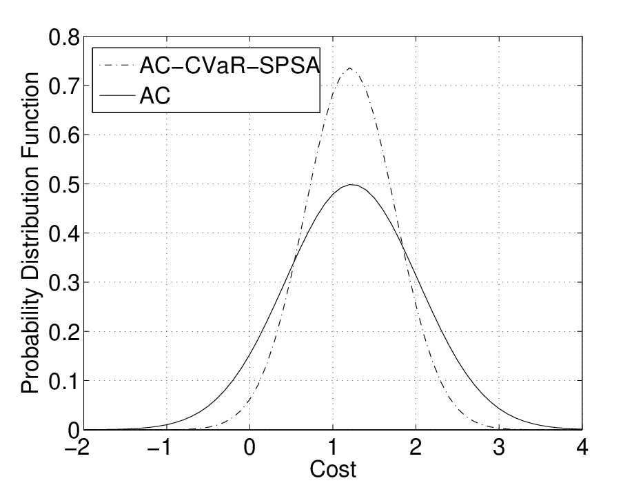
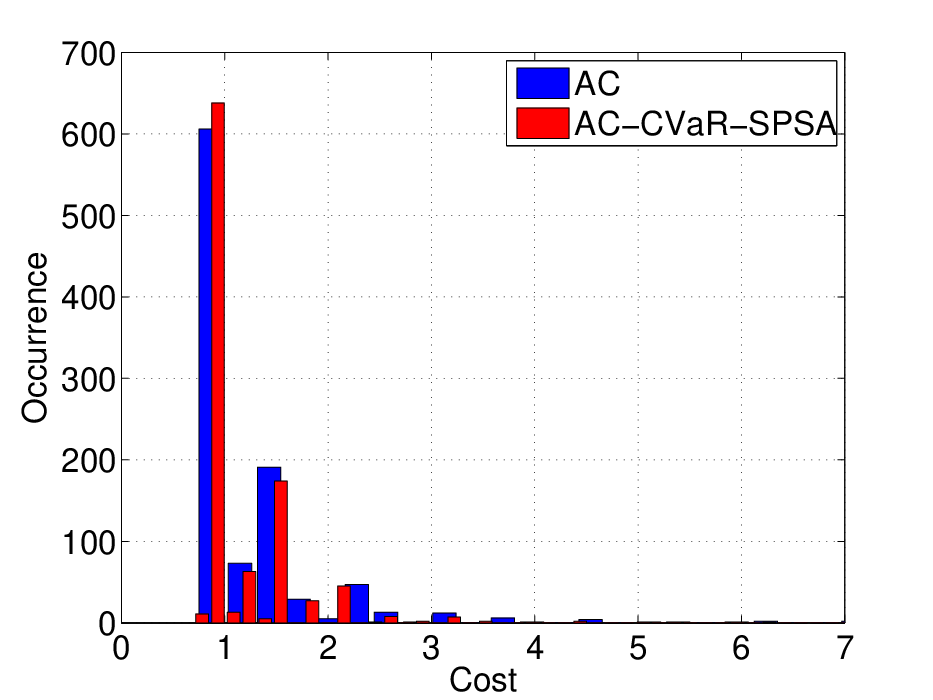
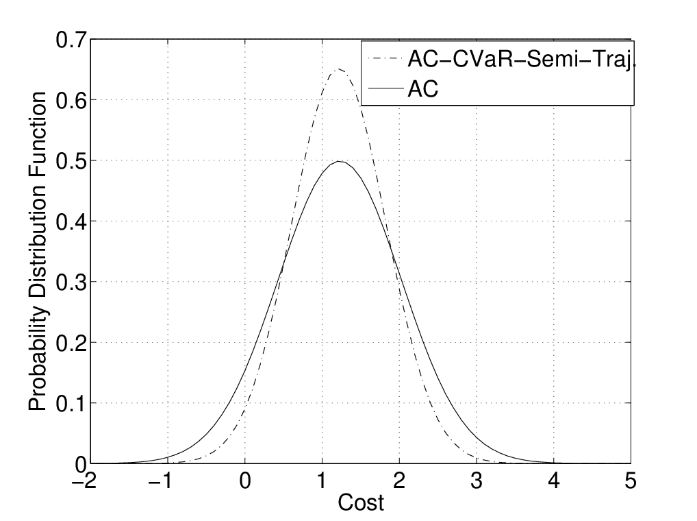
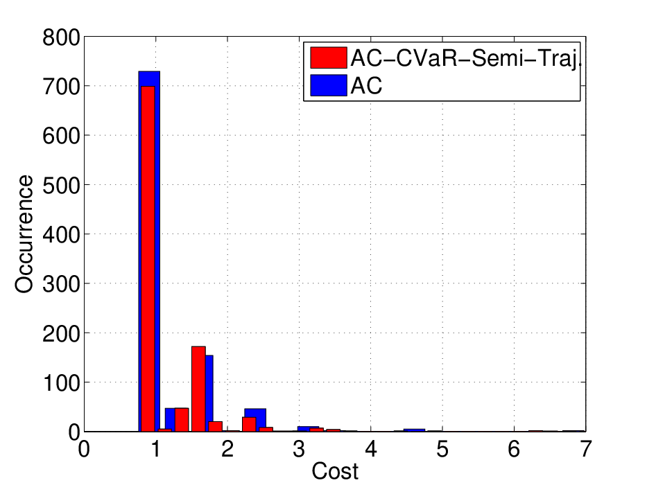
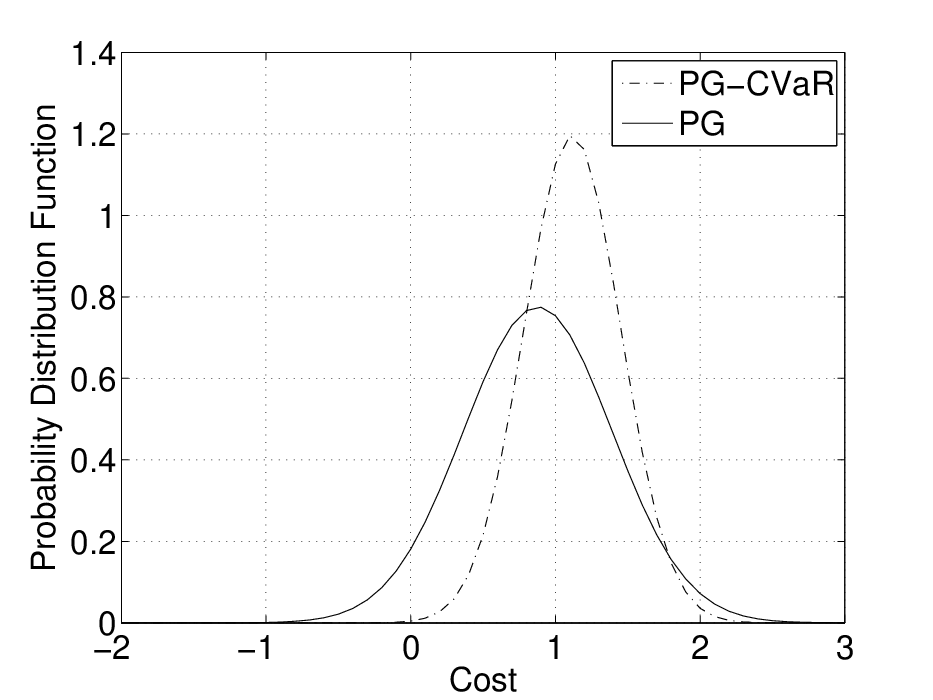
We compare the performance of our risk-sensitive policy gradient Alg. 1 (PG-CVaR) and two actor-critic Algs. 2 (AC-CVaR-SPSA,AC-CVaR-Semi-Traj) with their risk-neutral counterparts (PG and AC) (see Appendix C for the details of these experiments). Fig. 1 shows the distribution of the discounted cumulative cost Dθ​(x0)D^{\theta}(x^{0}) for the policy θ\theta learned by each of these algorithms. From left to right, the columns display the first two moments, the whole (distribution), and zoom on the right-tail of these distributions. The results indicate that the risk-sensitive algorithms yield a higher expected loss, but less variance, compared to the risk-neutral methods. More precisely, the loss distributions of the risk-sensitive algorithms have lower right-tail than their risk-neutral counterparts. Table 1 summarizes the performance of these algorithms. The numbers reiterate what we concluded from Fig. 1.
Refer to caption
Refer to caption
Refer to caption
Refer to caption
Refer to caption
Refer to caption
Refer to caption
Refer to caption
Refer to caption
Figure 1: Loss distributions for the policies learned by the risk-sensitive and risk-neutral algorithms.
𝔼⁡(Dθ​(x0))\mathbb{E}(D^{\theta}(x^{0})) σ2​(Dθ​(x0))\sigma^{2}(D^{\theta}(x^{0})) CVaR​(Dθ​(x0))\text{CVaR}(D^{\theta}(x^{0})) ℙ⁡(Dθ​(x0)≥β)\mathbb{P}(D^{\theta}(x^{0})\geq\beta)
PG 0.8780 0.2647 2.0855 0.058
PG-CVaR 1.1128 0.1109 1.7620 0.012
AC 1.1963 0.6399 2.6479 0.029
AC-CVaR-SPSA 1.2031 0.2942 2.3865 0.031
AC-CVaR-Semi-Traj. 1.2169 0.3747 2.3889 0.026
Table 1: Performance comparison for the policies learned by the risk-sensitive and risk-neutral algorithms.

7 Conclusions and Future Work

We proposed novel policy gradient and actor critic (AC) algorithms for CVaR optimization in MDPs. We provided proofs of convergence (in the appendix) to locally risk-sensitive optimal policies for the proposed algorithms. Further, using an optimal stopping problem, we observed that our algorithms resulted in policies whose loss distributions have lower right-tail compared to their risk-neutral counterparts. This is extremely important for a risk averse decision-maker, especially if the right-tail contains catastrophic losses. Future work includes: 1) Providing convergence proofs for our AC algorithms when the samples are generated by following the policy and not from its discounted visiting distribution (this can be wasteful in terms of samples), 2) Here we established asymptotic limits for our algorithms. To the best of our knowledge, there are no convergence rate results available for multi-timescale stochastic approximation schemes, and hence, for AC algorithms. This is true even for the AC algorithms that do not incorporate any risk criterion. It would be an interesting research direction to obtain finite-time bounds on the quality of the solution obtained by these algorithms, 3) Since interesting losses in the CVaR optimization problems are those that exceed the VaR, in order to compute more accurate estimates of the gradients, it is necessary to generate more samples in the right-tail of the loss distribution (events that are observed with a very low probability). Although importance sampling methods have been used to address this problem [3, 35], several issues, particularly related to the choice of the sampling distribution, have remained unsolved that are needed to be investigated, and finally, 4) Evaluating our algorithms in more challenging problems.

References

  • [1] Eitan Altman, Konstantin E Avrachenkov, and Rudesindo Núñez-Queija. Perturbation analysis for denumerable markov chains with application to queueing models. Advances in Applied Probability, pages 839–853, 2004.
  • [2] P. Artzner, F. Delbaen, J. Eber, and D. Heath. Coherent measures of risk. Journal of Mathematical Finance, 9(3):203–228, 1999.
  • [3] O. Bardou, N. Frikha, and G. Pagès. Computing VaR and CVaR using stochastic approximation and adaptive unconstrained importance sampling. Monte Carlo Methods and Applications, 15(3):173–210, 2009.
  • [4] N. Bäuerle and J. Ott. Markov decision processes with average-value-at-risk criteria. Mathematical Methods of Operations Research, 74(3):361–379, 2011.
  • [5] D. Bertsekas. Nonlinear programming. Athena Scientific, 1999.
  • [6] S. Bhatnagar. An actor-critic algorithm with function approximation for discounted cost constrained Markov decision processes. Systems & Control Letters, 59(12):760–766, 2010.
  • [7] S. Bhatnagar and K. Lakshmanan. An online actor-critic algorithm with function approximation for constrained Markov decision processes. Journal of Optimization Theory and Applications, pages 1–21, 2012.
  • [8] S. Bhatnagar, R. Sutton, M. Ghavamzadeh, and M. Lee. Natural actor-critic algorithms. Automatica, 45(11):2471–2482, 2009.
  • [9] S. Bhatnagar, H. Prasad, and L.A. Prashanth. Stochastic Recursive Algorithms for Optimization, volume 434. Springer, 2013.
  • [10] K. Boda and J. Filar. Time consistent dynamic risk measures. Mathematical Methods of Operations Research, 63(1):169–186, 2006.
  • [11] V. Borkar. A sensitivity formula for the risk-sensitive cost and the actor-critic algorithm. Systems & Control Letters, 44:339–346, 2001.
  • [12] V. Borkar. Q-learning for risk-sensitive control. Mathematics of Operations Research, 27:294–311, 2002.
  • [13] V. Borkar. An actor-critic algorithm for constrained Markov decision processes. Systems & Control Letters, 54(3):207–213, 2005.
  • [14] V. Borkar. Stochastic approximation: a dynamical systems viewpoint. Cambridge University Press, 2008.
  • [15] V. Borkar and R. Jain. Risk-constrained Markov decision processes. IEEE Transaction on Automatic Control, 2014.
  • [16] J. Filar, L. Kallenberg, and H. Lee. Variance-penalized Markov decision processes. Mathematics of Operations Research, 14(1):147–161, 1989.
  • [17] J. Filar, D. Krass, and K. Ross. Percentile performance criteria for limiting average Markov decision processes. IEEE Transaction of Automatic Control, 40(1):2–10, 1995.
  • [18] R. Howard and J. Matheson. Risk sensitive Markov decision processes. Management Science, 18(7):356–369, 1972.
  • [19] Hassan K Khalil and JW Grizzle. Nonlinear systems, volume 3. Prentice hall Upper Saddle River, 2002.
  • [20] Harold J Kushner and G George Yin. Stochastic approximation algorithms and applications. Springer, 1997.
  • [21] Prashanth L.A. and M. Ghavamzadeh. Actor-critic algorithms for risk-sensitive MDPs. In Proceedings of Advances in Neural Information Processing Systems 26, pages 252–260, 2013.
  • [22] H. Markowitz. Portfolio Selection: Efficient Diversification of Investment. John Wiley and Sons, 1959.
  • [23] Paul Milgrom and Ilya Segal. Envelope theorems for arbitrary choice sets. Econometrica, 70(2):583–601, 2002.
  • [24] T. Morimura, M. Sugiyama, M. Kashima, H. Hachiya, and T. Tanaka. Nonparametric return distribution approximation for reinforcement learning. In Proceedings of the 27th International Conference on Machine Learning, pages 799–806, 2010.
  • [25] J. Ott. A Markov Decision Model for a Surveillance Application and Risk-Sensitive Markov Decision Processes. PhD thesis, Karlsruhe Institute of Technology, 2010.
  • [26] J. Peters, S. Vijayakumar, and S. Schaal. Natural actor-critic. In Proceedings of the Sixteenth European Conference on Machine Learning, pages 280–291, 2005.
  • [27] M. Petrik and D. Subramanian. An approximate solution method for large risk-averse Markov decision processes. In Proceedings of the 28th International Conference on Uncertainty in Artificial Intelligence, 2012.
  • [28] R. Rockafellar and S. Uryasev. Conditional value-at-risk for general loss distributions. Journal of Banking and Finance, 2:s1–41, 2000.
  • [29] R. Rockafellar and S. Uryasev. Optimization of conditional value-at-risk. Journal of Risk, 26:1443–1471, 2002.
  • [30] EP Ryan. An integral invariance principle for differential inclusions with applications in adaptive control. SIAM Journal on Control and Optimization, 36(3):960–980, 1998.
  • [31] Tony Shardlow and Andrew M Stuart. A perturbation theory for ergodic markov chains and application to numerical approximations. SIAM journal on numerical analysis, 37(4):1120–1137, 2000.
  • [32] M. Sobel. The variance of discounted Markov decision processes. Applied Probability, pages 794–802, 1982.
  • [33] J. Spall. Multivariate stochastic approximation using a simultaneous perturbation gradient approximation. IEEE Transactions on Automatic Control, 37(3):332–341, 1992.
  • [34] A. Tamar, D. Di Castro, and S. Mannor. Policy gradients with variance related risk criteria. In Proceedings of the Twenty-Ninth International Conference on Machine Learning, pages 387–396, 2012.
  • [35] A. Tamar, Y. Glassner, and S. Mannor. Policy gradients beyond expectations: Conditional value-at-risk. arXiv:1404.3862v1, 2014.
  • [36] P. Thomas. Bias in natural actor-critic algorithms. In Proceedings of the Thirty-First International Conference on Machine Learning, 2014.

Appendix A Technical Details of the Trajectory-based Policy Gradient Algorithm

A.1 Assumptions

We make the following assumptions for the step-size schedules in our algorithms:

(A1) For any state-action pair (x,a)(x,a), μ⁡(a|x;θ)\mu(a|x;\theta) is continuously differentiable in θ\theta and ∇θμ​(a|x;θ)\nabla_{\theta}\mu(a|x;\theta) is a Lipschitz function in θ\theta for every a∈𝒜a\in\mathcal{A} and x∈𝒳x\in\mathcal{X}.

(A2) The Markov chain induced by any policy θ\theta is irreducible and aperiodic.

(A3) The step size schedules {ζ3​(i)}\{\zeta_{3}(i)\}, {ζ2​(i)}\{\zeta_{2}(i)\}, and {ζ1​(i)}\{\zeta_{1}(i)\} satisfy

∑iζ1​(i)=∑iζ2​(i)=∑iζ3​(i)=∞,\displaystyle\sum_{i}\zeta_{1}(i)=\sum_{i}\zeta_{2}(i)=\sum_{i}\zeta_{3}(i)=\infty, (23)
∑iζ1​(i)2,∑iζ2​(i)2,∑iζ3​(i)2<∞,\displaystyle\sum_{i}\zeta_{1}(i)^{2},\;\;\;\sum_{i}\zeta_{2}(i)^{2},\;\;\;\sum_{i}\zeta_{3}(i)^{2}<\infty, (24)
ζ1​(i)=o⁡(ζ2​(i)),ζ2​(i)=o⁡(ζ3​(i)).\displaystyle\zeta_{1}(i)=o\big(\zeta_{2}(i)\big),\;\;\;\zeta_{2}(i)=o\big(\zeta_{3}(i)\big). (25)

(23) and (24) are standard step-size conditions in stochastic approximation algorithms, and (25) indicates that the update corresponds to {ζ3​(i)}\{\zeta_{3}(i)\} is on the fastest time-scale, the update corresponds to {ζ2​(i)}\{\zeta_{2}(i)\} is on the intermediate time-scale, and the update corresponds to {ζ1​(i)}\{\zeta_{1}(i)\} is on the slowest time-scale.

A.2 Computing the Gradients

i) ∇θL​(θ,ν,λ)\nabla_{\theta}L(\theta,\nu,\lambda): Gradient of L⁡(θ,ν,λ)L(\theta,\nu,\lambda) w.r.t. θ\theta

By expanding the expectations in the definition of the objective function L⁡(θ,ν,λ)L(\theta,\nu,\lambda) in (4), we obtain

L⁡(θ,ν,λ)=∑ξℙθ​(ξ)​D​(ξ)+λ​ν+λ1−α​∑ξℙθ​(ξ)​(D⁡(ξ)−ν)+−λ​β.L(\theta,\nu,\lambda)=\sum_{\xi}\mathbb{P}_{\theta}(\xi)D(\xi)+\lambda\nu+\frac{\lambda}{1-\alpha}\sum_{\xi}\mathbb{P}_{\theta}(\xi)\big(D(\xi)-\nu\big)^{+}-\lambda\beta.

By taking gradient with respect to θ\theta, we have

∇θL​(θ,ν,λ)=∑ξ∇θℙθ​(ξ)​D​(ξ)+λ1−α​∑ξ∇θℙθ​(ξ)​(D⁡(ξ)−ν)+.\nabla_{\theta}L(\theta,\nu,\lambda)=\sum_{\xi}\nabla_{\theta}\mathbb{P}_{\theta}(\xi)D(\xi)+\frac{\lambda}{1-\alpha}\sum_{\xi}\nabla_{\theta}\mathbb{P}_{\theta}(\xi)\big(D(\xi)-\nu\big)^{+}.

This gradient can rewritten as

∇θL(θ,ν,λ)=∑ξℙθ(ξ)⋅∇θlogℙθ(ξ)(D(ξ)+λ1−α(D(ξ)−ν)𝟏{D(ξ)≥ν}),\nabla_{\theta}L(\theta,\nu,\lambda)=\sum_{\xi}\mathbb{P}_{\theta}(\xi)\cdot\nabla_{\theta}\log\mathbb{P}_{\theta}(\xi)\left(D(\xi)+\frac{\lambda}{1-\alpha}\big(D(\xi)-\nu\big)\mathbf{1}\big\{D(\xi)\geq\nu\big\}\right), (26)

where

∇θ​log​ℙθ​(ξ)=∇θ{∑k=0T−1logP(xk+1|xk,ak)+logμ(ak|xk;θ)+log𝟏{x0=x0}}=∑k=0T−11μ⁡(ak|xk;θ)​∇θμ​(ak|xk;θ)=∑k=0T−1∇θ​log​μ​(ak|xk;θ).\begin{split}\nabla_{\theta}\log\mathbb{P}_{\theta}(\xi)=&\nabla_{\theta}\left\{\sum_{k=0}^{T-1}\log P(x_{k+1}|x_{k},a_{k})+\log\mu(a_{k}|x_{k};\theta)+\log\mathbf{1}\{x_{0}=x^{0}\}\right\}\\ =&\sum_{k=0}^{T-1}\frac{1}{\mu(a_{k}|x_{k};\theta)}\nabla_{\theta}\mu(a_{k}|x_{k};\theta)\\ =&\sum_{k=0}^{T-1}\nabla_{\theta}\log\mu(a_{k}|x_{k};\theta).\end{split}

ii) ∂νL⁡(θ,ν,λ)\partial_{\nu}L(\theta,\nu,\lambda): Sub-differential of L⁡(θ,ν,λ)L(\theta,\nu,\lambda) w.r.t. ν\nu

From the definition of L⁡(θ,ν,λ)L(\theta,\nu,\lambda), we can easily see that L⁡(θ,ν,λ)L(\theta,\nu,\lambda) is a convex function in ν\nu for any fixed θ∈Θ\theta\in\Theta. Note that for every fixed ν\nu and any ν′\nu^{\prime}, we have

(D⁡(ξ)−ν′)+−(D⁡(ξ)−ν)+≥g⋅(ν′−ν),\big(D(\xi)-\nu^{\prime}\big)^{+}-\big(D(\xi)-\nu\big)^{+}\geq g\cdot(\nu^{\prime}-\nu),

where gg is any element in the set of sub-derivatives:

g∈∂ν(D(ξ)−ν)+=△{−1if ν<D⁡(ξ),−q:q∈[0,1]if ν=D⁡(ξ),0otherwise.g\in\partial_{\nu}\big(D(\xi)-\nu\big)^{+}\stackrel{{\scriptstyle\triangle}}{{=}}\begin{cases}-1&\text{if $\nu<D(\xi)$},\\ -q:q\in[0,1]&\text{if $\nu=D(\xi)$},\\ 0&\text{otherwise}.\end{cases}

Since L⁡(θ,ν,λ)L(\theta,\nu,\lambda) is finite-valued for any ν∈\nu\in\real, by the additive rule of sub-derivatives, we have

∂νL(θ,ν,λ)={−λ1−α∑ξℙθ(ξ)𝟏{D(ξ)>ν}−λ​q1−α∑ξℙθ(ξ)𝟏{D(ξ)=ν}+λ∣q∈[0,1]}.\partial_{\nu}L(\theta,\nu,\lambda)=\left\{-\frac{\lambda}{1-\alpha}\sum_{\xi}\mathbb{P}_{\theta}(\xi)\mathbf{1}\big\{D(\xi)>\nu\big\}-\frac{\lambda q}{1-\alpha}\sum_{\xi}\mathbb{P}_{\theta}(\xi)\mathbf{1}\big\{D(\xi)=\nu\big\}+\lambda\mid q\in[0,1]\right\}. (27)

In particular for q=1q=1, we may write the sub-gradient of L⁡(θ,ν,λ)L(\theta,\nu,\lambda) w.r.t. ν\nu as

∂νL(θ,ν,λ)|q=0=λ−λ1−α∑ξℙθ(ξ)⋅𝟏{D(ξ)≥ν}orλ−λ1−α∑ξℙθ(ξ)⋅𝟏{D(ξ)≥ν}∈∂νL(θ,ν,λ).\partial_{\nu}L(\theta,\nu,\lambda)|_{q=0}=\lambda-\frac{\lambda}{1-\alpha}\sum_{\xi}\mathbb{P}_{\theta}(\xi)\cdot\mathbf{1}\big\{D(\xi)\geq\nu\big\}\hskip 9.24994pt\text{or}\hskip 9.24994pt\lambda-\frac{\lambda}{1-\alpha}\sum_{\xi}\mathbb{P}_{\theta}(\xi)\cdot\mathbf{1}\big\{D(\xi)\geq\nu\big\}\in\partial_{\nu}L(\theta,\nu,\lambda).

iii) ∇λL​(θ,ν,λ)\nabla_{\lambda}L(\theta,\nu,\lambda): Gradient of L⁡(θ,ν,λ)L(\theta,\nu,\lambda) w.r.t. λ\lambda

Since L⁡(θ,ν,λ)L(\theta,\nu,\lambda) is a linear function in λ\lambda, obviously one can express the gradient of L⁡(θ,ν,λ)L(\theta,\nu,\lambda) w.r.t. λ\lambda as follows:

∇λL(θ,ν,λ)=ν−β+11−α∑ξℙθ(ξ)⋅(D(ξ)−ν)𝟏{D(ξ)≥ν}.\nabla_{\lambda}L(\theta,\nu,\lambda)=\nu-\beta+\frac{1}{1-\alpha}\sum_{\xi}\mathbb{P}_{\theta}(\xi)\cdot\big(D(\xi)-\nu\big)\mathbf{1}\big\{D(\xi)\geq\nu\big\}. (28)

A.3 Proof of Convergence of the Policy Gradient Algorithm

In this section, we prove the convergence of our policy gradient algorithm (Algorithm 1).

Theorem 2

Suppose λ∗∈[0,λmax)\lambda^{\ast}\in[0,\lambda_{\max}). Then the sequence of (θ,λ)−(\theta,\lambda)-updates in Algorithm 1 converges to a (local) saddle point (θ∗,ν∗,λ∗)(\theta^{*},\nu^{\ast},\lambda^{*}) of our objective function L⁡(θ,ν,λ)L(\theta,\nu,\lambda) almost surely, i.e., it satisfies L⁡(θ,ν,λ∗)≥L⁡(θ∗,ν∗,λ∗)≥L⁡(θ∗,ν∗,λ),∀(θ,ν)∈Θ×[−Cmax1−γ,Cmax1−γ]∩B(θ∗,ν∗)​(r)L(\theta,\nu,\lambda^{*})\geq L(\theta^{*},\nu^{\ast},\lambda^{*})\geq L(\theta^{*},\nu^{\ast},\lambda),\forall(\theta,\nu)\in\Theta\times[-\frac{C_{\max}}{1-\gamma},\frac{C_{\max}}{1-\gamma}]\cap B_{(\theta^{*},\nu^{*})}(r) for some r>0r>0 and ∀λ∈[0,λmax]\forall\lambda\in[0,\lambda_{\max}]. Note that B(θ∗,ν∗)​(r)B_{(\theta^{*},\nu^{*})}(r) represents a hyper-dimensional ball centered at (θ∗,ν∗)(\theta^{*},\nu^{*}) with radius rr.

Since ν\nu converges on the faster timescale than θ\theta and λ\lambda, the ν\nu-update can be rewritten by assuming (θ,λ)(\theta,\lambda) as invariant quantities, i.e.,

νi+1=ΓN[νi−ζ3(i)(λ−λ(1−α)​N∑j=1N𝟏{D(ξj,i)≥νi})].\nu_{i+1}=\Gamma_{N}\bigg[\nu_{i}-\zeta_{3}(i)\bigg(\lambda-\frac{\lambda}{(1-\alpha)N}\sum_{j=1}^{N}\mathbf{1}\big\{D(\xi_{j,i})\geq\nu_{i}\big\}\bigg)\bigg]. (29)

Consider the continuous time dynamics of ν\nu defined using differential inclusion

ν˙∈Υν​[−g⁡(ν)],∀g⁡(ν)∈∂νL⁡(θ,ν,λ),\dot{\nu}\in\Upsilon_{\nu}\left[-g(\nu)\right],\quad\quad\forall g(\nu)\in\partial_{\nu}L(\theta,\nu,\lambda), (30)

where

Υν​[K⁡(ν)]:=lim0<η→0ΓN​(ν+η​K​(ν))−ΓN​(ν)η.\Upsilon_{\nu}[K(\nu)]:=\lim_{0<\eta\rightarrow 0}\frac{\Gamma_{N}(\nu+\eta K(\nu))-\Gamma_{N}(\nu)}{\eta}.

and ΓN\Gamma_{N} is the Euclidean projection operator of ν\nu to [−Cmax1−γ,Cmax1−γ][-\frac{C_{\max}}{1-\gamma},\frac{C_{\max}}{1-\gamma}], i.e., ΓN​(ν)=arg⁡minν^∈[−Cmax1−γ,Cmax1−γ]​12​‖ν−ν^‖22\Gamma_{N}(\nu)=\arg\min_{\hat{\nu}\in[-\frac{C_{\max}}{1-\gamma},\frac{C_{\max}}{1-\gamma}]}\frac{1}{2}\|\nu-\hat{\nu}\|^{2}_{2}. In general ΓN​(ν)\Gamma_{N}(\nu) is not necessarily differentiable. Υν​[K​(ν)]\Upsilon_{\nu}[K(\nu)] is the left directional derivative of the function ΓN​(ν)\Gamma_{N}(\nu) in the direction of K⁡(ν)K(\nu). By using the left directional derivative Υν​[−g​(ν)]\Upsilon_{\nu}\left[-g(\nu)\right] in the sub-gradient descent algorithm for ν\nu, the gradient will point at the descent direction along the boundary of ν\nu whenever the ν−\nu-update hits its boundary.

Furthermore, since ν\nu converges on the faster timescale than θ\theta, and λ\lambda is on the slowest time-scale, the θ\theta-update can be rewritten using the converged ν∗​(θ)\nu^{*}(\theta) and assuming λ\lambda as an invariant quantity, i.e.,

θi+1=ΓΘ[θi−ζ2(i)(1N∑j=1N∇θlogℙθ(ξj,i)|θ=θiD(ξj,i)+λ(1−α)​N∑j=1N∇θlogℙθ(ξj,i)|θ=θi(D(ξj,i)−ν)𝟏{D(ξj,i)≥ν∗(θi)})].\begin{split}\theta_{i+1}=&\Gamma_{\Theta}\bigg[\theta_{i}-\zeta_{2}(i)\bigg(\frac{1}{N}\sum_{j=1}^{N}\nabla_{\theta}\log\mathbb{P}_{\theta}(\xi_{j,i})|_{\theta=\theta_{i}}D(\xi_{j,i})\\ &\hskip 52.39618pt+\frac{\lambda}{(1-\alpha)N}\sum_{j=1}^{N}\nabla_{\theta}\log\mathbb{P}_{\theta}(\xi_{j,i})|_{\theta=\theta_{i}}\big(D(\xi_{j,i})-\nu\big)\mathbf{1}\big\{D(\xi_{j,i})\geq\nu^{*}(\theta_{i})\big\}\bigg)\bigg].\end{split}

Consider the continuous time dynamics of θ∈Θ\theta\in\Theta:

θ˙=Υθ​[−∇θL​(θ,ν,λ)]|ν=ν∗​(θ),\dot{\theta}=\Upsilon_{\theta}\left[-\nabla_{\theta}L(\theta,\nu,\lambda)\right]|_{\nu=\nu^{*}(\theta)}, (31)

where

Υθ​[K⁡(θ)]:=lim0<η→0ΓΘ​(θ+η​K​(θ))−ΓΘ​(θ)η.\Upsilon_{\theta}[K(\theta)]:=\lim_{0<\eta\rightarrow 0}\frac{\Gamma_{\Theta}(\theta+\eta K(\theta))-\Gamma_{\Theta}(\theta)}{\eta}.

and ΓΘ\Gamma_{\Theta} is the Euclidean projection operator of θ\theta to Θ\Theta, i.e., ΓΘ​(θ)=arg⁡minθ^∈Θ​12​‖θ−θ^‖22\Gamma_{\Theta}(\theta)=\arg\min_{\hat{\theta}\in\Theta}\frac{1}{2}\|\theta-\hat{\theta}\|^{2}_{2}. Similar to the analysis of ν\nu, Υθ​[K​(θ)]\Upsilon_{\theta}[K(\theta)] is the left directional derivative of the function ΓΘ​(θ)\Gamma_{\Theta}(\theta) in the direction of K⁡(θ)K(\theta). By using the left directional derivative Υθ​[−∇θL​(θ,ν,λ)]\Upsilon_{\theta}\left[-\nabla_{\theta}L(\theta,\nu,\lambda)\right] in the gradient descent algorithm for θ\theta, the gradient will point at the descent direction along the boundary of Θ\Theta whenever the θ−\theta-update hits its boundary.

Finally, since λ\lambda-update converges in a slowest time-scale, the λ\lambda-update can be rewritten using the converged θ∗​(λ)\theta^{*}(\lambda) and ν∗​(λ)\nu^{*}(\lambda), i.e.,

λi+1=ΓΛ​(λi+ζ1​(i)​(ν∗​(λi)+11−α​1N​∑j=1N(D⁡(ξj,i)−ν∗​(λi))+−β)).\lambda_{i+1}=\Gamma_{\Lambda}\left(\lambda_{i}+\zeta_{1}(i)\bigg(\nu^{*}(\lambda_{i})+\frac{1}{1-\alpha}\frac{1}{N}\sum_{j=1}^{N}\big(D(\xi_{j,i})-\nu^{*}(\lambda_{i})\big)^{+}-\beta\bigg)\right). (32)

Consider the continuous time system

λ˙​(t)=Υλ​[∇λL​(θ,ν,λ)|θ=θ∗​(λ),ν=ν∗​(λ)],λ⁡(t)≥0,\dot{\lambda}(t)=\Upsilon_{\lambda}\left[\nabla_{\lambda}L(\theta,\nu,\lambda)\bigg|_{\theta=\theta^{*}(\lambda),\nu=\nu^{*}(\lambda)}\right],\quad\quad\lambda(t)\geq 0, (33)

where

Υλ​[K⁡(λ)]:=lim0<η→0ΓΛ​(λ+η​K​(λ))−ΓΛ​(λ)η.\Upsilon_{\lambda}[K(\lambda)]:=\lim_{0<\eta\rightarrow 0}\frac{\Gamma_{\Lambda}\big(\lambda+\eta K(\lambda)\big)-\Gamma_{\Lambda}(\lambda)}{\eta}.

and ΓΛ\Gamma_{\Lambda} is the Euclidean projection operator of λ\lambda to [0,λmax][0,\lambda_{\max}], i.e., ΓΛ​(λ)=arg⁡minλ^∈[0,λmax]​12​‖λ−λ^‖22\Gamma_{\Lambda}(\lambda)=\arg\min_{\hat{\lambda}\in[0,\lambda_{\max}]}\frac{1}{2}\|\lambda-\hat{\lambda}\|^{2}_{2}. Similar to the analysis of (ν,θ)(\nu,\theta), Υλ​[K​(λ)]\Upsilon_{\lambda}[K(\lambda)] is the left directional derivative of the function ΓΛ​(λ)\Gamma_{\Lambda}(\lambda) in the direction of K⁡(λ)K(\lambda). By using the left directional derivative Υλ​[∇λL​(θ,ν,λ)]\Upsilon_{\lambda}\left[\nabla_{\lambda}L(\theta,\nu,\lambda)\right] in the gradient ascent algorithm for λ\lambda, the gradient will point at the ascent direction along the boundary of [0,λmax][0,\lambda_{\max}] whenever the λ−\lambda-update hits its boundary.

Define

L∗​(λ)=L⁡(θ∗​(λ),ν∗​(λ),λ),L^{*}(\lambda)=L(\theta^{\ast}(\lambda),\nu^{\ast}(\lambda),\lambda),

for λ≥0\lambda\geq 0 where (θ∗​(λ),ν∗​(λ))∈Θ×[−Cmax1−γ,Cmax1−γ](\theta^{\ast}(\lambda),\nu^{\ast}(\lambda))\in\Theta\times[-\frac{C_{\max}}{1-\gamma},\frac{C_{\max}}{1-\gamma}] is a local minimum of L⁡(θ,ν,λ)L(\theta,\nu,\lambda) for fixed λ≥0\lambda\geq 0, i.e., L⁡(θ,ν,λ)≥L⁡(θ∗​(λ),ν∗​(λ),λ)L(\theta,\nu,\lambda)\geq L(\theta^{\ast}(\lambda),\nu^{\ast}(\lambda),\lambda) for any (θ,ν)∈Θ×[−Cmax1−γ,Cmax1−γ]∩B(θ∗​(λ),ν∗​(λ))​(r)(\theta,\nu)\in\Theta\times[-\frac{C_{\max}}{1-\gamma},\frac{C_{\max}}{1-\gamma}]\cap B_{(\theta^{\ast}(\lambda),\nu^{\ast}(\lambda))}(r) for some r>0r>0.

Next, we want to show that the ODE (33) is actually a gradient ascent of the Lagrangian function using the envelope theorem in mathematical economics [23]. The envelope theorem describes sufficient conditions for the derivative of L∗L^{*} with respect to λ\lambda where it equals to the partial derivative of the objective function LL with respect to λ\lambda, holding (θ,ν)(\theta,\nu) at its local optimum (θ,ν)=(θ∗​(λ),ν∗​(λ))(\theta,\nu)=(\theta^{\ast}(\lambda),\nu^{\ast}(\lambda)). We will show that ∇λL∗​(λ)\nabla_{\lambda}L^{\ast}(\lambda) coincides with with ∇λL​(θ,ν,λ)|θ=θ∗​(λ),ν=ν∗​(λ)\nabla_{\lambda}L(\theta,\nu,\lambda)|_{\theta=\theta^{\ast}(\lambda),\nu=\nu^{\ast}(\lambda)} as follows.

Theorem 3

The value function L∗L^{*} is absolutely continuous. Furthermore,

L∗​(λ)=L∗​(0)+∫0λ∇λ′L​(θ,ν,λ′)|θ=θ∗​(s),ν=ν∗​(s),λ′=s​𝑑s,λ≥0.L^{*}(\lambda)=L^{*}(0)+\int_{0}^{\lambda}\nabla_{\lambda^{\prime}}L(\theta,\nu,\lambda^{\prime})\Big|_{\theta=\theta^{*}(s),\nu=\nu^{*}(s),\lambda^{\prime}=s}ds,\,\,\lambda\geq 0. (34)

Proof. The proof follows from analogous arguments of Lemma 4.3 in [13]. From the definition of L∗L^{*}, observe that for any λ′,λ′′≥0\lambda^{\prime},\lambda^{\prime\prime}\geq 0 with λ′<λ′′\lambda^{\prime}<\lambda^{\prime\prime},

|L∗​(λ′′)−L∗​(λ′)|≤supθ∈Θ,ν∈[−Cmax1−γ,Cmax1−γ]|L⁡(θ,ν,λ′′)−L⁡(θ,ν,λ′)|=supθ∈Θ,ν∈[−Cmax1−γ,Cmax1−γ]|∫λ′λ′′∇λL​(θ,ν,s)​ds|≤∫λ′λ′′supθ∈Θ,ν∈[−Cmax1−γ,Cmax1−γ]|∇λL​(θ,ν,s)|​ds≤3​Cmax(1−α)​(1−γ)​(λ′′−λ′).\small\begin{split}|L^{*}(\lambda^{\prime\prime})-L^{*}(\lambda^{\prime})|\leq&\sup_{\theta\in\Theta,\nu\in[-\frac{C_{\max}}{1-\gamma},\frac{C_{\max}}{1-\gamma}]}|L(\theta,\nu,\lambda^{\prime\prime})-L(\theta,\nu,\lambda^{\prime})|\\ =&\sup_{\theta\in\Theta,\nu\in[-\frac{C_{\max}}{1-\gamma},\frac{C_{\max}}{1-\gamma}]}\left|\int_{\lambda^{\prime}}^{\lambda^{\prime\prime}}\nabla_{\lambda}L(\theta,\nu,s)ds\right|\\ \leq&\int_{\lambda^{\prime}}^{\lambda^{\prime\prime}}\sup_{\theta\in\Theta,\nu\in[\frac{-C_{\max}}{1-\gamma},\frac{C_{\max}}{1-\gamma}]}\left|\nabla_{\lambda}L(\theta,\nu,s)\right|ds\leq\frac{3C_{\max}}{(1-\alpha)(1-\gamma)}(\lambda^{\prime\prime}-\lambda^{\prime}).\end{split}

This implies that L∗L^{*} is absolutely continuous. Therefore, L∗L^{*} is continuous everywhere and differentiable almost everywhere.

By the Milgrom-Segal envelope theorem of mathematical economics (Theorem 1 of [23]), one can conclude that the derivative of L∗​(λ)L^{*}(\lambda) coincides with the derivative of L⁡(θ,ν,λ)L(\theta,\nu,\lambda) at the point of differentiability λ\lambda and θ=θ∗​(λ)\theta=\theta^{*}(\lambda), ν=ν∗​(λ)\nu=\nu^{*}(\lambda). Also since L∗L^{*} is absolutely continuous, the limit of (L∗​(λ)−L∗​(λ′))/(λ−λ′)(L^{*}(\lambda)-L^{*}(\lambda^{\prime}))/(\lambda-\lambda^{\prime}) at λ↑λ′\lambda\uparrow\lambda^{\prime} (or λ↓λ′\lambda\downarrow\lambda^{\prime}) coincides with the lower/upper directional derivatives if λ′\lambda^{\prime} is a point of non-differentiability. Thus, there is only a countable number of non-differentiable points in L∗L^{*} and each point of non-differentiability has the same directional derivatives as the point slightly beneath (in the case of λ↓λ′\lambda\downarrow\lambda^{\prime}) or above (in the case of λ↑λ′\lambda\uparrow\lambda^{\prime}) it. As the set of non-differentiable points of L∗L^{*} has measure zero, it can then be interpreted that ∇λL∗​(λ)\nabla_{\lambda}L^{\ast}(\lambda) coincides with ∇λL​(θ,ν,λ)|θ=θ∗​(λ),ν=ν∗​(λ)\nabla_{\lambda}L(\theta,\nu,\lambda)|_{\theta=\theta^{*}(\lambda),\nu=\nu^{*}(\lambda)}, i.e., expression (34) holds. ■\blacksquare

Remark 1

It can be easily shown that L∗​(λ)L^{*}(\lambda) is a concave function. Since for given θ\theta and ν\nu, L⁡(θ,ν,λ)L(\theta,\nu,\lambda) is a linear function in λ\lambda. Therefore, for any α′∈[0,1]\alpha^{\prime}\in[0,1], α′​L∗​(λ1)+(1−α′)​L∗​(λ2)≤L∗​(α′​λ1+(1−α′)​λ2)\alpha^{\prime}L^{*}(\lambda_{1})+(1-\alpha^{\prime})L^{*}(\lambda_{2})\leq L^{*}(\alpha^{\prime}\lambda_{1}+(1-\alpha^{\prime})\lambda_{2}), i.e., L∗​(λ)L^{*}(\lambda) is a concave function. Concavity of L∗L^{*} implies that it is continuous and directionally (both left hand and right hand) differentiable in int dom​(L∗)\text{int dom}(L^{*}). Furthermore at any λ=λ~\lambda=\tilde{\lambda} such that the derivative of L⁡(θ,ν,λ)L(\theta,\nu,\lambda) with respect of λ\lambda at θ=θ∗​(λ),ν=ν∗​(λ)\theta=\theta^{*}(\lambda),\nu=\nu^{*}(\lambda) exists, by Theorem 1 of [23], ∇λL∗​(λ)|λ=λ~+=(L∗​(λ~+)−L∗​(λ~))/(λ~+−λ~)≥∇λL​(θ,ν,λ)|θ=θ∗​(λ),ν=ν∗​(λ),λ=λ~≥(L∗​(λ~−)−L∗​(λ~))/(λ~−−λ~)=∇λL∗​(λ)|λ=λ~−\nabla_{\lambda}L^{*}(\lambda)|_{\lambda=\tilde{\lambda}_{+}}=(L^{*}(\tilde{\lambda}_{+})-L^{*}(\tilde{\lambda}))/(\tilde{\lambda}_{+}-\tilde{\lambda})\geq\nabla_{\lambda}L(\theta,\nu,\lambda)|_{\theta=\theta^{*}(\lambda),\nu=\nu^{*}(\lambda),\lambda=\tilde{\lambda}}\geq(L^{*}(\tilde{\lambda}_{-})-L^{*}(\tilde{\lambda}))/(\tilde{\lambda}_{-}-\tilde{\lambda})=\nabla_{\lambda}L^{*}(\lambda)|_{\lambda=\tilde{\lambda}_{-}}. Furthermore concavity of L∗L^{*} implies ∇λL∗​(λ)|λ=λ~+≤∇λL∗​(λ)|λ=λ~−\nabla_{\lambda}L^{*}(\lambda)|_{\lambda=\tilde{\lambda}_{+}}\leq\nabla_{\lambda}L^{*}(\lambda)|_{\lambda=\tilde{\lambda}_{-}}. Combining these arguments, one obtains ∇λL∗​(λ)|λ=λ~+=∇λL​(θ,ν,λ)|θ=θ∗​(λ),ν=ν∗​(λ),λ=λ~=∇λL∗​(λ)|λ=λ~−\nabla_{\lambda}L^{*}(\lambda)|_{\lambda=\tilde{\lambda}_{+}}=\nabla_{\lambda}L(\theta,\nu,\lambda)|_{\theta=\theta^{*}(\lambda),\nu=\nu^{*}(\lambda),\lambda=\tilde{\lambda}}=\nabla_{\lambda}L^{*}(\lambda)|_{\lambda=\tilde{\lambda}_{-}}.

In order to prove the main convergence result, we need the following standard assumptions and remarks.

Assumption 4

For any given x0∈𝒳x^{0}\in\mathcal{X} and θ∈Θ\theta\in\Theta, the set {(ν,g⁡(ν))∣g⁡(ν)∈∂νL⁡(θ,ν,λ)}\big\{\big(\nu,g(\nu)\big)\mid g(\nu)\in\partial_{\nu}L(\theta,\nu,\lambda)\big\} is closed.

Remark 2

For any given θ∈Θ\theta\in\Theta, λ≥0\lambda\geq 0, and g⁡(ν)∈∂νL⁡(θ,ν,λ)g(\nu)\in\partial_{\nu}L(\theta,\nu,\lambda), we have

|g⁡(ν)|≤3​λ​(1+|ν|)/(1−α).|g(\nu)|\leq 3\lambda(1+|\nu|)/(1-\alpha). (35)

To see this, recall from definition that gg can be parameterized by qq as, for q∈[0,1]q\in[0,1],

g(ν)=−λ(1−α)∑ξℙθ(ξ)𝟏{D(ξ)>ν}−λ​q1−α∑ξℙθ(ξ)𝟏{D(ξ)=ν}+λ.g(\nu)=-\frac{\lambda}{(1-\alpha)}\sum_{\xi}\mathbb{P}_{\theta}(\xi)\mathbf{1}\left\{D(\xi)>\nu\right\}-\frac{\lambda q}{1-\alpha}\sum_{\xi}\mathbb{P}_{\theta}(\xi)\mathbf{1}\left\{D(\xi)=\nu\right\}+\lambda.

It is obvious that |𝟏{D(ξ)=ν}|,|𝟏{D(ξ)>ν}|≤1+|ν|\left|\mathbf{1}\left\{D(\xi)=\nu\right\}\right|,\left|\mathbf{1}\left\{D(\xi)>\nu\right\}\right|\leq 1+|\nu|. Thus, |∑ξℙθ(ξ)𝟏{D(ξ)>ν}|≤supξ|𝟏{D(ξ)>ν}|≤1+|ν|\left|\sum_{\xi}\mathbb{P}_{\theta}(\xi)\mathbf{1}\left\{D(\xi)>\nu\right\}\right|\leq\sup_{\xi}\left|\mathbf{1}\left\{D(\xi)>\nu\right\}\right|\leq 1+|\nu|, and |∑ξℙθ(ξ)𝟏{D(ξ)=ν}|≤1+|ν|\left|\sum_{\xi}\mathbb{P}_{\theta}(\xi)\mathbf{1}\left\{D(\xi)=\nu\right\}\right|\leq 1+|\nu|. Recalling 0<(1−q),(1−α)<10<(1-q),\,(1-\alpha)<1, these arguments imply the claim of (35).

Before getting into the main result, we need the following technical proposition.

Proposition 5

∇θL​(θ,ν,λ)\nabla_{\theta}L(\theta,\nu,\lambda) is Lipschitz in θ\theta.

Proof. Recall that

∇θL(θ,ν,λ)=∑ξℙθ(ξ)⋅∇θlogℙθ(ξ)(D(ξ)+λ1−α(D(ξ)−ν)𝟏{D(ξ)≥ν})\nabla_{\theta}L(\theta,\nu,\lambda)=\sum_{\xi}\mathbb{P}_{\theta}(\xi)\cdot\nabla_{\theta}\log\mathbb{P}_{\theta}(\xi)\left(D(\xi)+\frac{\lambda}{1-\alpha}\big(D(\xi)-\nu\big)\mathbf{1}\big\{D(\xi)\geq\nu\big\}\right)

and ∇θ​log​ℙθ​(ξ)=∑k=0T−1∇θμ​(ak|xk;θ)/μ⁡(ak|xk;θ)\nabla_{\theta}\log\mathbb{P}_{\theta}(\xi)=\sum_{k=0}^{T-1}\nabla_{\theta}\mu(a_{k}|x_{k};\theta)/\mu(a_{k}|x_{k};\theta) whenever μ⁡(ak|xk;θ)∈(0,1]\mu(a_{k}|x_{k};\theta)\in(0,1]. Now Assumption (A1) implies that ∇θμ​(ak|xk;θ)\nabla_{\theta}\mu(a_{k}|x_{k};\theta) is a Lipschitz function in θ\theta for any a∈𝒜a\in\mathcal{A} and k∈{0,…,T−1}k\in\{0,\ldots,T-1\} and μ⁡(ak|xk;θ)\mu(a_{k}|x_{k};\theta) is differentiable in θ\theta. Therefore, by recalling that ℙθ(ξ)=∏k=0T−1P(xk+1|xk,ak)μ(ak|xk;θ)𝟏{x0=x0}\mathbb{P}_{\theta}(\xi)=\prod_{k=0}^{T-1}P(x_{k+1}|x_{k},a_{k})\mu(a_{k}|x_{k};\theta)\mathbf{1}\{x_{0}=x^{0}\} and by combining these arguments and noting that the sum of products of Lipschitz functions is Lipschitz, one concludes that ∇θL​(θ,ν,λ)\nabla_{\theta}L(\theta,\nu,\lambda) is Lipschitz in θ\theta. ■\blacksquare

Remark 3

∇θL​(θ,ν,λ)\nabla_{\theta}L(\theta,\nu,\lambda) is Lipschitz in θ\theta implies that ‖∇θL​(θ,ν,λ)‖2≤2​(‖∇θL​(θ0,ν,λ)‖+‖θ0‖)2+2​‖θ‖2\|\nabla_{\theta}L(\theta,\nu,\lambda)\|^{2}\leq 2(\|\nabla_{\theta}L(\theta_{0},\nu,\lambda)\|+\|\theta_{0}\|)^{2}+2\|\theta\|^{2} which further implies that

‖∇θL​(θ,ν,λ)‖2≤K1​(1+‖θ‖2).\|\nabla_{\theta}L(\theta,\nu,\lambda)\|^{2}\leq K_{1}(1+\|\theta\|^{2}).

for K1=2​max⁡(1,(‖∇θL​(θ0,ν,λ)‖+‖θ0‖)2)>0K_{1}=2\max(1,(\|\nabla_{\theta}L(\theta_{0},\nu,\lambda)\|+\|\theta_{0}\|)^{2})>0. Similarly, ∇θ​log​ℙθ​(ξ)\nabla_{\theta}\log\mathbb{P}_{\theta}(\xi) is Lipschitz implies that

‖∇θ​log​ℙθ​(ξ)‖2≤K2​(ξ)​(1+‖θ‖2).\|\nabla_{\theta}\log\mathbb{P}_{\theta}(\xi)\|^{2}\leq K_{2}(\xi)(1+\|\theta\|^{2}).

for a positive random variable K2​(ξ)K_{2}(\xi). Furthermore, since T<∞T<\infty w.p. 11, μ⁡(ak|xk;θ)∈(0,1]\mu(a_{k}|x_{k};\theta)\in(0,1] and ∇θμ​(ak|xk;θ)\nabla_{\theta}\mu(a_{k}|x_{k};\theta) is Lipschitz for any k<Tk<T, K2​(ξ)<∞K_{2}(\xi)<\infty w.p. 11.

We are now in a position to prove the convergence analysis of Theorem 2.

Proof. [Proof of Theorem 2] We split the proof into the following four steps:

Step 1 (Convergence of ν−\nu-update)

Since ν\nu converges in a faster time scale than θ\theta and λ\lambda, one can assume both θ\theta and λ\lambda as fixed quantities in the ν\nu-update, i.e.,

νi+1=ΓN(νi+ζ3(i)(λ(1−α)​N∑j=1N𝟏{D(ξj,i)≥νi}−λ+δνi+1)),\nu_{i+1}=\Gamma_{N}\left(\nu_{i}+\zeta_{3}(i)\left(\frac{\lambda}{(1-\alpha)N}\sum_{j=1}^{N}\mathbf{1}\big\{D(\xi_{j,i})\geq\nu_{i}\big\}-\lambda+\delta\nu_{i+1}\right)\right), (36)

and

δνi+1=λ1−α(−1N∑j=1N𝟏{D(ξj,i)≥νi}+∑ξℙθ(ξ)𝟏{D(ξ)≥νi}).\delta\nu_{i+1}=\frac{\lambda}{1-\alpha}\left(-\frac{1}{N}\sum_{j=1}^{N}\mathbf{1}\big\{D(\xi_{j,i})\geq\nu_{i}\big\}+\sum_{\xi}\mathbb{P}_{\theta}(\xi)\mathbf{1}\{D(\xi)\geq\nu_{i}\}\right). (37)

First, one can show that δ​νi+1\delta\nu_{i+1} is square integrable, i.e.

𝔼⁡[‖δ​νi+1‖2∣Fν,i]≤4​(λmax1−α)2\mathbb{E}[\|\delta\nu_{i+1}\|^{2}\mid F_{\nu,i}]\leq 4\left(\frac{\lambda_{\max}}{1-\alpha}\right)^{2}

where ℱν,i=σ⁡(νm,δ​νm,m≤i)\mathcal{F}_{\nu,i}=\sigma\big(\nu_{m},\,\delta\nu_{m},\,m\leq i\big) is the filtration of νi\nu_{i} generated by different independent trajectories.

Second, since the history trajectories are generated based on the sampling probability mass function ℙθ​(ξ)\mathbb{P}_{\theta}(\xi), expression (27) implies that 𝔼⁡[δ​νi+1∣ℱν,i]=0\mathbb{E}\left[\delta\nu_{i+1}\mid\mathcal{F}_{\nu,i}\right]=0. Therefore, the ν\nu-update is a stochastic approximation of the ODE (30) with a Martingale difference error term, i.e.,

λ1−α∑ξℙθ(ξ)𝟏{D(ξ)≥νi}−λ∈−∂νL(θ,ν,λ)|ν=νi.\frac{\lambda}{1-\alpha}\sum_{\xi}\mathbb{P}_{\theta}(\xi)\mathbf{1}\{D(\xi)\geq\nu_{i}\}-\lambda\in-\partial_{\nu}L(\theta,\nu,\lambda)|_{\nu=\nu_{i}}.

Then one can invoke Corollary 4 in Chapter 5 of [14] (stochastic approximation theory for non-differentiable systems) to show that the sequence {νi},νi∈[−Cmax1−γ,Cmax1−γ]\{\nu_{i}\},\;\nu_{i}\in[-\frac{C_{\max}}{1-\gamma},\frac{C_{\max}}{1-\gamma}] converges almost surely to a fixed point ν∗∈[−Cmax1−γ,Cmax1−γ]\nu^{*}\in[-\frac{C_{\max}}{1-\gamma},\frac{C_{\max}}{1-\gamma}] of differential inclusion (31), where ν∗∈Nc:={ν∈[−Cmax1−γ,Cmax1−γ]:Υν[−g(ν)]=0,g(ν)∈∂νL(θ,ν,λ)}\nu^{\ast}\in N_{c}:=\{\nu\in[-\frac{C_{\max}}{1-\gamma},\frac{C_{\max}}{1-\gamma}]:\Upsilon_{\nu}[-g(\nu)]=0,\,g(\nu)\in\partial_{\nu}L(\theta,\nu,\lambda)\}. To justify the assumptions of this theorem, 1) from Remark 2, the Lipschitz property is satisfied, i.e., supg⁡(ν)∈∂νL⁡(θ,ν,λ)|g⁡(ν)|≤3​λ​(1+|ν|)/(1−α)\sup_{g(\nu)\in\partial_{\nu}L(\theta,\nu,\lambda)}|g(\nu)|\leq 3\lambda(1+|\nu|)/(1-\alpha), 2) ∂νL⁡(θ,ν,λ)\partial_{\nu}L(\theta,\nu,\lambda) is a convex compact set by definition, 3) Assumption 4 implies that {(ν,g⁡(ν))∣g⁡(ν)∈∂νL⁡(θ,ν,λ)}\{(\nu,g(\nu))\mid g(\nu)\in\partial_{\nu}L(\theta,\nu,\lambda)\} is a closed set. This implies ∂νL⁡(θ,ν,λ)\partial_{\nu}L(\theta,\nu,\lambda) is an upper semi-continuous set valued mapping 4) the step-size rule follows from (A.1), 5) the Martingale difference assumption follows from (37), and 6) νi∈[−Cmax1−γ,Cmax1−γ]\nu_{i}\in[-\frac{C_{\max}}{1-\gamma},\frac{C_{\max}}{1-\gamma}], ∀i\forall i implies that supi‖νi‖<∞\sup_{i}\|\nu_{i}\|<\infty almost surely.

Consider the ODE of ν∈\nu\in\real in (30), we define the set-valued derivative of LL as follows:

Dt​L​(θ,ν,λ)={g⁡(ν)​Υν​[−g⁡(ν)]∣∀g⁡(ν)∈∂νL⁡(θ,ν,λ)}.D_{t}L(\theta,\nu,\lambda)=\big\{g(\nu)\Upsilon_{\nu}\big[-g(\nu)\big]\mid\forall g(\nu)\in\partial_{\nu}L(\theta,\nu,\lambda)\big\}.

One may conclude that

maxg⁡(ν)⁡Dt​L​(θ,ν,λ)=max⁡{g⁡(ν)​Υν​[−g⁡(ν)]∣g⁡(ν)∈∂νL⁡(θ,ν,λ)}.\max_{g(\nu)}D_{t}L(\theta,\nu,\lambda)=\max\big\{g(\nu)\Upsilon_{\nu}\big[-g(\nu)\big]\mid g(\nu)\in\partial_{\nu}L(\theta,\nu,\lambda)\big\}.

We have the following cases:

Case 1: When ν∈(−Cmax1−γ,Cmax1−γ)\nu\in(-\frac{C_{\max}}{1-\gamma},\frac{C_{\max}}{1-\gamma}).
For every g⁡(ν)∈∂νL⁡(θ,ν,λ)g(\nu)\in\partial_{\nu}L(\theta,\nu,\lambda), there exists a sufficiently small η0>0\eta_{0}>0 such that ν−η0​g​(ν)∈[−Cmax1−γ,Cmax1−γ]\nu-\eta_{0}g(\nu)\in[-\frac{C_{\max}}{1-\gamma},\frac{C_{\max}}{1-\gamma}] and

ΓN​(θ−η0​g​(ν))−θ=−η0​g​(ν).\Gamma_{N}\big(\theta-\eta_{0}g(\nu)\big)-\theta=-\eta_{0}g(\nu).

Therefore, the definition of Υθ​[−g​(ν)]\Upsilon_{\theta}[-g(\nu)] implies

maxg⁡(ν)⁡Dt​L​(θ,ν,λ)=max⁡{−g2​(ν)∣g⁡(ν)∈∂νL⁡(θ,ν,λ)}≤0.\max_{g(\nu)}D_{t}L(\theta,\nu,\lambda)=\max\big\{-g^{2}(\nu)\mid g(\nu)\in\partial_{\nu}L(\theta,\nu,\lambda)\big\}\leq 0. (38)

The maximum is attained because ∂νL⁡(θ,ν,λ)\partial_{\nu}L(\theta,\nu,\lambda) is a convex compact set and g⁡(ν)​Υν​[−g⁡(ν)]g(\nu)\Upsilon_{\nu}\big[-g(\nu)\big] is a continuous function. At the same time, we have maxg⁡(ν)⁡Dt​L​(θ,ν,λ)<0\max_{g(\nu)}D_{t}L(\theta,\nu,\lambda)<0 whenever 0∉∂νL⁡(θ,ν,λ)0\not\in\partial_{\nu}L(\theta,\nu,\lambda).

Case 2: When ν∈{−Cmax1−γ,Cmax1−γ}\nu\in\{-\frac{C_{\max}}{1-\gamma},\frac{C_{\max}}{1-\gamma}\} and for any g⁡(ν)∈∂Lν​(θ,ν,λ)g(\nu)\in\partial L_{\nu}(\theta,\nu,\lambda) such that ν−η​g​(ν)∈[−Cmax1−γ,Cmax1−γ]\nu-\eta g(\nu)\in[-\frac{C_{\max}}{1-\gamma},\frac{C_{\max}}{1-\gamma}], for any η∈(0,η0]\eta\in(0,\eta_{0}] and some η0>0\eta_{0}>0.
The condition ν−η​g​(ν)∈[−Cmax1−γ,Cmax1−γ]\nu-\eta g(\nu)\in[-\frac{C_{\max}}{1-\gamma},\frac{C_{\max}}{1-\gamma}] implies that

Υν​[−g⁡(ν)]=−g⁡(ν).\Upsilon_{\nu}\big[-g(\nu)\big]=-g(\nu).

Then we obtain

maxg⁡(ν)⁡Dt​L​(θ,ν,λ)=max⁡{−g2​(ν)∣g⁡(ν)∈∂νL⁡(θ,ν,λ)}≤0.\max_{g(\nu)}D_{t}L(\theta,\nu,\lambda)=\max\big\{-g^{2}(\nu)\mid g(\nu)\in\partial_{\nu}L(\theta,\nu,\lambda)\big\}\leq 0. (39)

Furthermore, we have maxg⁡(ν)⁡Dt​L​(θ,ν,λ)<0\max_{g(\nu)}D_{t}L(\theta,\nu,\lambda)<0 whenever 0∉∂νL⁡(θ,ν,λ)0\not\in\partial_{\nu}L(\theta,\nu,\lambda).

Case 3: When ν∈{−Cmax1−γ,Cmax1−γ}\nu\in\{-\frac{C_{\max}}{1-\gamma},\frac{C_{\max}}{1-\gamma}\} and there exists a non-empty set 𝒢(ν):={g(ν)∈∂Lν(θ,ν,λ)∣θ−ηg(ν)∉[−Cmax1−γ,Cmax1−γ],∃η∈(0,η0],∀η0>0}\mathcal{G}(\nu):=\{g(\nu)\in\partial L_{\nu}(\theta,\nu,\lambda)\mid\theta-\eta g(\nu)\not\in[-\frac{C_{\max}}{1-\gamma},\frac{C_{\max}}{1-\gamma}],\,\exists\eta\in(0,\eta_{0}],\,\forall\eta_{0}>0\}.
First, consider any g⁡(ν)∈𝒢⁡(ν)g(\nu)\in\mathcal{G}(\nu). For any η>0\eta>0, define νη:=ν−η​g​(ν)\nu_{\eta}:=\nu-\eta g(\nu). The above condition implies that when 0<η→00<\eta\rightarrow 0, ΓN​[νη]\Gamma_{N}\big[\nu_{\eta}\big] is the projection of νη\nu_{\eta} to the tangent space of [−Cmax1−γ,Cmax1−γ][-\frac{C_{\max}}{1-\gamma},\frac{C_{\max}}{1-\gamma}]. For any elements ν^∈[−Cmax1−γ,Cmax1−γ]\hat{\nu}\in[-\frac{C_{\max}}{1-\gamma},\frac{C_{\max}}{1-\gamma}], since the following set {ν∈[−Cmax1−γ,Cmax1−γ]:‖ν−νη‖2≤‖ν^−νη‖2}\{\nu\in[-\frac{C_{\max}}{1-\gamma},\frac{C_{\max}}{1-\gamma}]:\|\nu-\nu_{\eta}\|_{2}\leq\|\hat{\nu}-\nu_{\eta}\|_{2}\} is compact, the projection of νη\nu_{\eta} on [−Cmax1−γ,Cmax1−γ][-\frac{C_{\max}}{1-\gamma},\frac{C_{\max}}{1-\gamma}] exists. Furthermore, since f⁡(ν):=12​(ν−νη)2f(\nu):=\frac{1}{2}(\nu-\nu_{\eta})^{2} is a strongly convex function and ∇f​(ν)=ν−νη\nabla f(\nu)=\nu-\nu_{\eta}, by first order optimality condition, one obtains

∇f​(νη∗)​(ν−νη∗)=(νη∗−νη)​(ν−νη∗)≥0,∀ν∈[−Cmax1−γ,Cmax1−γ]\nabla f(\nu_{\eta}^{\ast})(\nu-\nu_{\eta}^{\ast})=(\nu_{\eta}^{\ast}-\nu_{\eta})(\nu-\nu_{\eta}^{\ast})\geq 0,\quad\forall\nu\in\left[-\frac{C_{\max}}{1-\gamma},\frac{C_{\max}}{1-\gamma}\right]

where νη∗\nu_{\eta}^{\ast} is an unique projection of νη\nu_{\eta} (the projection is unique because f⁡(ν)f(\nu) is strongly convex and [−Cmax1−γ,Cmax1−γ][-\frac{C_{\max}}{1-\gamma},\frac{C_{\max}}{1-\gamma}] is a convex compact set). Since the projection (minimizer) is unique, the above equality holds if and only if ν=νη∗\nu=\nu_{\eta}^{\ast}.

Therefore, for any ν∈[−Cmax1−γ,Cmax1−γ]\nu\in[-\frac{C_{\max}}{1-\gamma},\frac{C_{\max}}{1-\gamma}] and η>0\eta>0,

g⁡(ν)​Υν​[−g⁡(ν)]=g⁡(ν)​(lim0<η→0νη∗−νη)=(lim0<η→0ν−νηη)​(lim0<η→0νη∗−νη)=lim0<η→0−‖νη∗−ν‖2η2+lim0<η→0(νη∗−νη)​(νη∗−νη2)≤0.\begin{split}&g(\nu)\Upsilon_{\nu}\big[-g(\nu)\big]=g(\nu)\left(\lim_{0<\eta\rightarrow 0}\frac{\nu_{\eta}^{\ast}-\nu}{\eta}\right)\\ =&\left(\lim_{0<\eta\rightarrow 0}\frac{\nu-\nu_{\eta}}{\eta}\right)\left(\lim_{0<\eta\rightarrow 0}\frac{\nu_{\eta}^{\ast}-\nu}{\eta}\right)=\lim_{0<\eta\rightarrow 0}\frac{-\|\nu_{\eta}^{\ast}-\nu\|^{2}}{\eta^{2}}+\lim_{0<\eta\rightarrow 0}\big(\nu_{\eta}^{\ast}-\nu_{\eta}\big)\left(\frac{\nu_{\eta}^{\ast}-\nu}{\eta^{2}}\right)\leq 0.\end{split}

Second, for any g⁡(ν)∈∂νL⁡(θ,ν,λ)∩𝒢​(ν)cg(\nu)\in\partial_{\nu}L(\theta,\nu,\lambda)\cap\mathcal{G}(\nu)^{c}, one obtains ν−η​g​(ν)∈[−Cmax1−γ,Cmax1−γ]\nu-\eta g(\nu)\in[-\frac{C_{\max}}{1-\gamma},\frac{C_{\max}}{1-\gamma}], for any η∈(0,η0]\eta\in(0,\eta_{0}] and some η0>0\eta_{0}>0. In this case, the arguments follow from case 2 and the following expression holds, Υν​[−g⁡(ν)]=−g⁡(ν)\Upsilon_{\nu}\big[-g(\nu)\big]=-g(\nu).

Combining these arguments, one concludes that

maxg⁡(ν)⁡Dt​L​(θ,ν,λ)≤max⁡{max⁡{g⁡(ν)​Υν​[−g⁡(ν)]∣g⁡(ν)∈𝒢⁡(ν)},max⁡{−g2​(ν)∣g⁡(ν)∈∂νL⁡(θ,ν,λ)∩𝒢​(ν)c}}≤0.\small\begin{split}&\max_{g(\nu)}D_{t}L(\theta,\nu,\lambda)\\ \leq&\max\left\{\max\big\{g(\nu)\;\Upsilon_{\nu}\big[-g(\nu)\big]\mid g(\nu)\in\mathcal{G}(\nu)\big\},\max\big\{-g^{2}(\nu)\mid g(\nu)\in\partial_{\nu}L(\theta,\nu,\lambda)\cap\mathcal{G}(\nu)^{c}\big\}\right\}\leq 0.\end{split} (40)

This quantity is non-zero whenever 0∉{g⁡(ν)​Υν​[−g⁡(ν)]∣∀g⁡(ν)∈∂νL⁡(θ,ν,λ)}0\not\in\{g(\nu)\;\Upsilon_{\nu}\big[-g(\nu)\big]\mid\forall g(\nu)\in\partial_{\nu}L(\theta,\nu,\lambda)\} (this is because, for any g⁡(ν)∈∂νL⁡(θ,ν,λ)∩𝒢​(ν)cg(\nu)\in\partial_{\nu}L(\theta,\nu,\lambda)\cap\mathcal{G}(\nu)^{c}, one obtains g⁡(ν)​Υν​[−g⁡(ν)]=−g​(ν)2g(\nu)\;\Upsilon_{\nu}\big[-g(\nu)\big]=-g(\nu)^{2}).

Thus, by similar arguments one may conclude that maxg⁡(ν)⁡Dt​L​(θ,ν,λ)≤0\max_{g(\nu)}D_{t}L(\theta,\nu,\lambda)\leq 0 and it is non-zero if Υν​[−g⁡(ν)]≠0\Upsilon_{\nu}\big[-g(\nu)\big]\neq 0 for every g⁡(ν)∈∂νL⁡(θ,ν,λ)g(\nu)\in\partial_{\nu}L(\theta,\nu,\lambda). Therefore, by Lasalle’s invariance principle for differential inclusion (see Theorem 2.11 [30]), the above arguments imply that with any initial condition θ⁡(0)\theta(0), the state trajectory ν⁡(t)\nu(t) of (31) converges to a stable stationary point ν∗\nu^{\ast} in the positive invariant set NcN_{c}. Since maxg⁡(ν)⁡Dt​L​(θ,ν,λ)≤0\max_{g(\nu)}D_{t}L(\theta,\nu,\lambda)\leq 0, ν˙\dot{\nu} is a descent direction of L⁡(θ,ν,λ)L(\theta,\nu,\lambda) for fixed θ\theta and λ\lambda, i.e., L⁡(θ,ν∗,λ)≤L⁡(θ,ν⁡(t),λ)≤L⁡(θ,ν⁡(0),λ)L(\theta,\nu^{\ast},\lambda)\leq L(\theta,\nu(t),\lambda)\leq L(\theta,\nu(0),\lambda) for any t≥0t\geq 0.

Step 2 (Convergence of θ−\theta-update)

Since θ\theta converges in a faster time scale than λ\lambda and ν\nu converges faster than θ\theta, one can assume λ\lambda as a fixed quantity and ν\nu as a converged quantity ν∗​(θ)\nu^{*}(\theta) in the θ\theta-update. The θ\theta-update can be rewritten as a stochastic approximation, i.e.,

θi+1=ΓΘ​(θi+ζ2​(i)​(−∇θL​(θ,ν,λ)|θ=θi,ν=ν∗​(θi)+δ​θi+1)),\theta_{i+1}=\Gamma_{\Theta}\left(\theta_{i}+\zeta_{2}(i)\bigg(-\nabla_{\theta}L(\theta,\nu,\lambda)|_{\theta=\theta_{i},\nu=\nu^{*}(\theta_{i})}+\delta\theta_{i+1}\bigg)\right), (41)

where

δ​θi+1=∇θL​(θ,ν,λ)|θ=θi,ν=ν∗​(θi)−1N​∑j=1N∇θ​log​ℙθ​(ξj,i)∣θ=θi​D​(ξj,i)−λ(1−α)​N∑j=1N∇θlogℙθ(ξj,i)|θ=θi(D(ξj,i)−ν∗(θi))𝟏{D(ξj,i)≥ν∗(θi)}.\begin{split}\delta\theta_{i+1}=&\nabla_{\theta}L(\theta,\nu,\lambda)|_{\theta=\theta_{i},\nu=\nu^{*}(\theta_{i})}\!-\!\frac{1}{N}\sum_{j=1}^{N}\nabla_{\theta}\log\mathbb{P}_{\theta}(\xi_{j,i})\mid_{\theta=\theta_{i}}D(\xi_{j,i})\\ &-\frac{\lambda}{(1-\alpha)N}\sum_{j=1}^{N}\nabla_{\theta}\log\mathbb{P}_{\theta}(\xi_{j,i})|_{\theta=\theta_{i}}\big(D(\xi_{j,i})-\nu^{*}(\theta_{i})\big)\mathbf{1}\big\{D(\xi_{j,i})\geq\nu^{*}(\theta_{i})\big\}.\end{split} (42)

First, one can show that δ​θi+1\delta\theta_{i+1} is square integrable, i.e., 𝔼⁡[‖δ​θi+1‖2∣Fθ,i]≤Ki​(1+‖θi‖2)\mathbb{E}[\|\delta\theta_{i+1}\|^{2}\mid F_{\theta,i}]\leq K_{i}(1+\|\theta_{i}\|^{2}) for some Ki>0K_{i}>0, where ℱθ,i=σ⁡(θm,δ​θm,m≤i)\mathcal{F}_{\theta,i}=\sigma\big(\theta_{m},\,\delta\theta_{m},\,m\leq i\big) is the filtration of θi\theta_{i} generated by different independent trajectories. To see this, notice that

‖δ​θi+1‖2≤2​(∇θL​(θ,ν,λ)|θ=θi,ν=ν∗​(θi))2+2N2​(Cmax1−γ+2​λ​Cmax(1−α)​(1−γ))2​(∑j=1N∇θ​log​ℙθ​(ξj,i)∣θ=θi)2≤2​K1,i​(1+‖θi‖2)+2NN2​(Cmax1−γ+2​λmax​Cmax(1−α)​(1−γ))2​(∑j=1N‖∇θ​log​ℙθ​(ξj,i)∣θ=θi‖2)≤2​K1,i​(1+‖θi‖2)+2NN2​(Cmax1−γ+2​λmax​Cmax(1−α)​(1−γ))2​(∑j=1NK2​(ξj,i)​(1+‖θi‖2))≤(K1,i+2N−1N​(Cmax1−γ+2​λmax​Cmax(1−α)​(1−γ))2​max1≤j≤N​K2​(ξj,i))​(+‖θi‖2)\small\begin{split}\|\delta\theta_{i+1}\|^{2}\leq&2\left(\nabla_{\theta}L(\theta,\nu,\lambda)|_{\theta=\theta_{i},\nu=\nu^{*}(\theta_{i})}\right)^{2}+\frac{2}{N^{2}}\left(\frac{C_{\max}}{1-\gamma}+\frac{2\lambda C_{\max}}{(1-\alpha)(1-\gamma)}\right)^{2}\left(\sum_{j=1}^{N}\nabla_{\theta}\log\mathbb{P}_{\theta}(\xi_{j,i})\mid_{\theta=\theta_{i}}\right)^{2}\\ \leq&2K_{1,i}(1+\|\theta_{i}\|^{2})+\frac{2^{N}}{N^{2}}\left(\frac{C_{\max}}{1-\gamma}+\frac{2\lambda_{\max}C_{\max}}{(1-\alpha)(1-\gamma)}\right)^{2}\left(\sum_{j=1}^{N}\left\|\nabla_{\theta}\log\mathbb{P}_{\theta}(\xi_{j,i})\mid_{\theta=\theta_{i}}\right\|^{2}\right)\\ \leq&2K_{1,i}(1+\|\theta_{i}\|^{2})+\frac{2^{N}}{N^{2}}\left(\frac{C_{\max}}{1-\gamma}+\frac{2\lambda_{\max}C_{\max}}{(1-\alpha)(1-\gamma)}\right)^{2}\left(\sum_{j=1}^{N}K_{2}(\xi_{j,i})(1+\|\theta_{i}\|^{2})\right)\\ \leq&2\!\left(K_{1,i}\!+\!\frac{2^{N-1}}{N}\left(\frac{C_{\max}}{1-\gamma}+\frac{2\lambda_{\max}C_{\max}}{(1-\alpha)(1-\gamma)}\right)^{2}\max_{1\leq j\leq N}K_{2}(\xi_{j,i})\right)\!(1\!+\!\|\theta_{i}\|^{2})\end{split}

The Lipschitz upper bounds are due to results in Remark 3. Since K2​(ξj,i)<∞K_{2}(\xi_{j,i})<\infty w.p. 11, there exists K2,i<∞K_{2,i}<\infty such that max1≤j≤N⁡K2​(ξj,i)≤K2,i\max_{1\leq j\leq N}K_{2}(\xi_{j,i})\leq K_{2,i}. Furthermore, T<∞T<\infty w.p. 11 implies 𝔼⁡[T2∣ℱθ,i]<∞\mathbb{E}[T^{2}\mid\mathcal{F}_{\theta,i}]<\infty. By combining these results, one concludes that 𝔼⁡[‖δ​θi+1‖2∣Fθ,i]≤Ki​(+‖θi‖2)\mathbb{E}[\|\delta\theta_{i+1}\|^{2}\mid F_{\theta,i}]\leq K_{i}(1\!+\!\|\theta_{i}\|^{2}) where

Ki=2​(K1,i+2N−1​K2,iN​(Cmax1−γ+2​λmax​Cmax(1−α)​(1−γ))2)<∞.K_{i}=2\left(K_{1,i}\!+\!\frac{2^{N-1}K_{2,i}}{N}\left(\frac{C_{\max}}{1-\gamma}+\frac{2\lambda_{\max}C_{\max}}{(1-\alpha)(1-\gamma)}\right)^{2}\right)<\infty.

Second, since the history trajectories are generated based on the sampling probability mass function ℙθi​(ξ)\mathbb{P}_{\theta_{i}}(\xi), expression (26) implies that 𝔼⁡[δ​θi+1∣ℱθ,i]=0\mathbb{E}\left[\delta\theta_{i+1}\mid\mathcal{F}_{\theta,i}\right]=0. Therefore, the θ\theta-update is a stochastic approximation of the ODE (31) with a Martingale difference error term. In addition, from the convergence analysis of ν−\nu-update, ν∗​(θ)\nu^{\ast}(\theta) is an asymptotically stable equilibrium point of {νi}\{\nu_{i}\}. From (27), ∂νL⁡(θ,ν,λ)\partial_{\nu}L(\theta,\nu,\lambda) is a Lipschitz set-valued mapping in θ\theta (since ℙθ​(ξ)\mathbb{P}_{\theta}(\xi) is Lipschitz in θ\theta), it can be easily seen that ν∗​(θ)\nu^{\ast}(\theta) is a Lipschitz continuous mapping of θ\theta.

Now consider the continuous time system θ∈Θ\theta\in\Theta in (31). We may write

d​L​(θ,ν,λ)d​t|ν=ν∗​(θ)=(∇θL​(θ,ν,λ)|ν=ν∗​(θ))⊤​Υθ​[−∇θL​(θ,ν,λ)|ν=ν∗​(θ)].\frac{dL(\theta,\nu,\lambda)}{dt}\bigg|_{\nu=\nu^{*}(\theta)}=\big(\nabla_{\theta}L(\theta,\nu,\lambda)|_{\nu=\nu^{*}(\theta)}\big)^{\top}\;\Upsilon_{\theta}\big[-\nabla_{\theta}L(\theta,\nu,\lambda)|_{\nu=\nu^{*}(\theta)}\big]. (43)

We have the following cases:

Case 1: When θ∈Θ∘\theta\in\Theta^{\circ}.
Since Θ∘\Theta^{\circ} is the interior of the set Θ\Theta and Θ\Theta is a convex compact set, there exists a sufficiently small η0>0\eta_{0}>0 such that θ−η0​∇θL​(θ,ν,λ)|ν=ν∗​(θ)∈Θ\theta-\eta_{0}\nabla_{\theta}L(\theta,\nu,\lambda)|_{\nu=\nu^{*}(\theta)}\in\Theta and

ΓΘ​(θ−η0​∇θL​(θ,ν,λ)|ν=ν∗​(θ))−θ=−η0​∇θL​(θ,ν,λ)|ν=ν∗​(θ).\Gamma_{\Theta}\big(\theta-\eta_{0}\nabla_{\theta}L(\theta,\nu,\lambda)|_{\nu=\nu^{*}(\theta)}\big)-\theta=-\eta_{0}\nabla_{\theta}L(\theta,\nu,\lambda)|_{\nu=\nu^{*}(\theta)}.

Therefore, the definition of Υθ​[−∇θL​(θ,ν,λ)|ν=ν∗​(θ)]\Upsilon_{\theta}\big[-\nabla_{\theta}L(\theta,\nu,\lambda)|_{\nu=\nu^{*}(\theta)}\big] implies

d​L​(θ,ν,λ)d​t|ν=ν∗​(θ)=−‖∇θL​(θ,ν,λ)|ν=ν∗​(θ)‖2≤0.\frac{dL(\theta,\nu,\lambda)}{dt}\bigg|_{\nu=\nu^{*}(\theta)}=-\left\|\nabla_{\theta}L(\theta,\nu,\lambda)|_{\nu=\nu^{*}(\theta)}\right\|^{2}\leq 0. (44)

At the same time, we have d​L​(θ,ν,λ)/d​t|ν=ν∗​(θ)<0{dL(\theta,\nu,\lambda)}/{dt}|_{\nu=\nu^{*}(\theta)}<0 whenever ‖∇θL​(θ,ν,λ)|ν=ν∗​(θ)‖≠0\|\nabla_{\theta}L(\theta,\nu,\lambda)|_{\nu=\nu^{*}(\theta)}\|\neq 0.

Case 2: When θ∈∂Θ\theta\in\partial\Theta and θ−η​∇θL​(θ,ν,λ)|ν=ν∗​(θ)∈Θ\theta-\eta\nabla_{\theta}L(\theta,\nu,\lambda)|_{\nu=\nu^{*}(\theta)}\in\Theta for any η∈(0,η0]\eta\in(0,\eta_{0}] and some η0>0\eta_{0}>0.
The condition θ−η​∇θL​(θ,ν,λ)|ν=ν∗​(θ)∈Θ\theta-\eta\nabla_{\theta}L(\theta,\nu,\lambda)|_{\nu=\nu^{*}(\theta)}\in\Theta implies that

Υθ​[−∇θL​(θ,ν,λ)|ν=ν∗​(θ)]=−∇θL​(θ,ν,λ)|ν=ν∗​(θ).\Upsilon_{\theta}\big[-\nabla_{\theta}L(\theta,\nu,\lambda)|_{\nu=\nu^{*}(\theta)}\big]=-\nabla_{\theta}L(\theta,\nu,\lambda)|_{\nu=\nu^{*}(\theta)}.

Then we obtain

d​L​(θ,ν,λ)d​t|ν=ν∗​(θ)=−‖∇θL​(θ,ν,λ)|ν=ν∗​(θ)‖2≤0.\begin{split}\frac{dL(\theta,\nu,\lambda)}{dt}\bigg|_{\nu=\nu^{*}(\theta)}=-\left\|\nabla_{\theta}L(\theta,\nu,\lambda)|_{\nu=\nu^{*}(\theta)}\right\|^{2}\leq 0.\end{split} (45)

Furthermore, d​L​(θ,ν,λ)/d​t|ν=ν∗​(θ)<0{dL(\theta,\nu,\lambda)}/{dt}|_{\nu=\nu^{*}(\theta)}<0 when ‖∇θL​(θ,ν,λ)|ν=ν∗​(θ)‖≠0\|\nabla_{\theta}L(\theta,\nu,\lambda)|_{\nu=\nu^{*}(\theta)}\|\neq 0.

Case 3: When θ∈∂Θ\theta\in\partial\Theta and θ−η​∇θL​(θ,ν,λ)|ν=ν∗​(θ)∉Θ\theta-\eta\nabla_{\theta}L(\theta,\nu,\lambda)|_{\nu=\nu^{*}(\theta)}\not\in\Theta for some η∈(0,η0]\eta\in(0,\eta_{0}] and any η0>0\eta_{0}>0.
For any η>0\eta>0, define θη:=θ−η​∇θL​(θ,ν,λ)|ν=ν∗​(θ)\theta_{\eta}:=\theta-\eta\nabla_{\theta}L(\theta,\nu,\lambda)|_{\nu=\nu^{*}(\theta)}. The above condition implies that when 0<η→00<\eta\rightarrow 0, ΓΘ​[θη]\Gamma_{\Theta}\big[\theta_{\eta}\big] is the projection of θη\theta_{\eta} to the tangent space of Θ\Theta. For any elements θ^∈Θ\hat{\theta}\in\Theta, since the following set {θ∈Θ:‖θ−θη‖2≤‖θ^−θη‖2}\{\theta\in\Theta:\|\theta-\theta_{\eta}\|_{2}\leq\|\hat{\theta}-\theta_{\eta}\|_{2}\} is compact, the projection of θη\theta_{\eta} on Θ\Theta exists. Furthermore, since f⁡(θ):=12​‖θ−θη‖22f(\theta):=\frac{1}{2}\|\theta-\theta_{\eta}\|_{2}^{2} is a strongly convex function and ∇f​(θ)=θ−θη\nabla f(\theta)=\theta-\theta_{\eta}, by first order optimality condition, one obtains

∇f(θη∗)⊤(θ−θη∗)=(θη∗−θη)⊤(θ−θη∗)≥0,∀θ∈Θ\nabla f(\theta_{\eta}^{\ast})^{\top}(\theta-\theta_{\eta}^{\ast})=(\theta_{\eta}^{\ast}-\theta_{\eta})^{\top}(\theta-\theta_{\eta}^{\ast})\geq 0,\quad\forall\theta\in\Theta

where θη∗\theta_{\eta}^{\ast} is an unique projection of θη\theta_{\eta} (the projection is unique because f⁡(θ)f(\theta) is strongly convex and Θ\Theta is a convex compact set). Since the projection (minimizer) is unique, the above equality holds if and only if θ=θη∗\theta=\theta_{\eta}^{\ast}.

Therefore, for any θ∈Θ\theta\in\Theta and η>0\eta>0,

(∇θL​(θ,ν,λ)|ν=ν∗​(θ))⊤​Υθ​[−∇θL​(θ,ν,λ)|ν=ν∗​(θ)]=(∇θL​(θ,ν,λ)|ν=ν∗​(θ))⊤​(lim0<η→0θη∗−θη)=(lim0<η→0θ−θηη)⊤​(lim0<η→0θη∗−θη)=lim0<η→0−‖θη∗−θ‖2η2+lim0<η→0(θη∗−θη)⊤​(θη∗−θη2)≤0.\begin{split}&\big(\nabla_{\theta}L(\theta,\nu,\lambda)|_{\nu=\nu^{*}(\theta)}\big)^{\top}\;\Upsilon_{\theta}\big[-\nabla_{\theta}L(\theta,\nu,\lambda)|_{\nu=\nu^{*}(\theta)}\big]=\big(\nabla_{\theta}L(\theta,\nu,\lambda)|_{\nu=\nu^{*}(\theta)}\big)^{\top}\left(\lim_{0<\eta\rightarrow 0}\frac{\theta_{\eta}^{\ast}-\theta}{\eta}\right)\\ =&\left(\lim_{0<\eta\rightarrow 0}\frac{\theta-\theta_{\eta}}{\eta}\right)^{\top}\left(\lim_{0<\eta\rightarrow 0}\frac{\theta_{\eta}^{\ast}-\theta}{\eta}\right)=\lim_{0<\eta\rightarrow 0}\frac{-\|\theta_{\eta}^{\ast}-\theta\|^{2}}{\eta^{2}}+\lim_{0<\eta\rightarrow 0}\big(\theta_{\eta}^{\ast}-\theta_{\eta}\big)^{\top}\left(\frac{\theta_{\eta}^{\ast}-\theta}{\eta^{2}}\right)\leq 0.\end{split}

From these arguments, one concludes that d​L​(θ,ν,λ)/d​t|ν=ν∗​(θ)≤0{dL(\theta,\nu,\lambda)}/{dt}|_{\nu=\nu^{*}(\theta)}\leq 0 and this quantity is non-zero whenever ‖Υθ​[−∇θL​(θ,ν,λ)|ν=ν∗​(θ)]‖≠0\left\|\Upsilon_{\theta}\left[-\nabla_{\theta}L(\theta,\nu,\lambda)|_{\nu=\nu^{*}(\theta)}\right]\right\|\neq 0.

Therefore, by Lasalle’s invariance principle [19], the above arguments imply that with any initial condition θ⁡(0)\theta(0), the state trajectory θ⁡(t)\theta(t) of (31) converges to a stable stationary point θ∗\theta^{\ast} in the positive invariant set Θc\Theta_{c} and L⁡(θ∗,ν∗​(θ∗),λ)≤L⁡(θ⁡(t),ν∗​(θ⁡(t)),λ)≤L⁡(θ⁡(0),ν∗​(θ⁡(0)),λ)L(\theta^{\ast},\nu^{\ast}(\theta^{\ast}),\lambda)\leq L(\theta(t),\nu^{\ast}(\theta(t)),\lambda)\leq L(\theta(0),\nu^{\ast}(\theta(0)),\lambda) for any t≥0t\geq 0.

Based on the above properties and noting that 1) from Proposition 5, ∇θL​(θ,ν,λ)\nabla_{\theta}L(\theta,\nu,\lambda) is a Lipschitz function in θ\theta, 2) the step-size rule follows from Section A.1, 3) expression (47) implies that δ​θi+1\delta\theta_{i+1} is a square integrable Martingale difference, and 4) θi∈Θ\theta_{i}\in\Theta, ∀i\forall i implies that supi‖θi‖<∞\sup_{i}\|\theta_{i}\|<\infty almost surely, one can invoke Theorem 2 in Chapter 6 of [14] (multi-time scale stochastic approximation theory) to show that the sequence {θi},θi∈Θ\{\theta_{i}\},\;\theta_{i}\in\Theta converges almost surely to a fixed point θ∗∈Θ\theta^{*}\in\Theta of ODE (31), where θ∗∈Θc:={θ∈Θ:Υθ​[−∇θL​(θ,ν,λ)|ν=ν∗​(θ)]=0}\theta^{\ast}\in\Theta_{c}:=\{\theta\in\Theta:\Upsilon_{\theta}[-\nabla_{\theta}L(\theta,\nu,\lambda)|_{\nu=\nu^{*}(\theta)}]=0\}. Also, it can be easily seen that Θc\Theta_{c} is a closed subset of the compact set Θ\Theta, which is a compact set as well.

Step 3 (Local Minimum)

Now, we want to show that {θi,νi}\{\theta_{i},\nu_{i}\} converges to a local minimum of L⁡(θ,ν,λ)L(\theta,\nu,\lambda) for fixed λ\lambda. Recall {θi,νi}\{\theta_{i},\nu_{i}\} converges to (θ∗,ν∗):=(θ∗,ν∗​(θ∗))(\theta^{\ast},\nu^{\ast}):=(\theta^{\ast},\nu^{\ast}(\theta^{\ast})). From previous arguments on (ν,θ)(\nu,\theta) convergence analysis imply that with any initial condition (θ⁡(0),ν⁡(0))(\theta(0),\nu(0)), the state trajectories θ⁡(t)\theta(t) and OPENν⁡(t))\nu(t)) of (30) and (31) converge to the set of stationary points (θ∗,ν∗)(\theta^{\ast},\nu^{\ast}) in the positive invariant set Θc×Nc\Theta_{c}\times N_{c} and L⁡(θ∗,ν∗,λ)≤L⁡(θ⁡(t),ν∗​(θ⁡(t)),λ)≤L⁡(θ⁡(0),ν∗​(θ⁡(0)),λ)≤L⁡(θ⁡(0),ν⁡(t),λ)≤L⁡(θ⁡(0),ν⁡(0),λ)L(\theta^{\ast},\nu^{\ast},\lambda)\leq L(\theta(t),\nu^{\ast}(\theta(t)),\lambda)\leq L(\theta(0),\nu^{\ast}(\theta(0)),\lambda)\leq L(\theta(0),\nu(t),\lambda)\leq L(\theta(0),\nu(0),\lambda) for any t≥0t\geq 0.

By contradiction, suppose (θ∗,ν∗)(\theta^{\ast},\nu^{\ast}) is not a local minimum. Then there exists (θ¯,ν¯)∈Θ×[−Cmax1−γ,Cmax1−γ]∩B(θ∗,ν∗)​(r)(\bar{\theta},\bar{\nu})\in\Theta\times[-\frac{C_{\max}}{1-\gamma},\frac{C_{\max}}{1-\gamma}]\cap B_{(\theta^{\ast},\nu^{\ast})}(r) such that L⁡(θ¯,ν¯,λ)=min(θ,ν)∈Θ×[−Cmax1−γ,Cmax1−γ]∩B(θ∗,ν∗)​(r)⁡L⁡(θ,ν,λ)L(\bar{\theta},\bar{\nu},\lambda)=\min_{(\theta,\nu)\in\Theta\times[-\frac{C_{\max}}{1-\gamma},\frac{C_{\max}}{1-\gamma}]\cap B_{(\theta^{\ast},\nu^{\ast})}(r)}L(\theta,\nu,\lambda). The minimum is attained by Weierstrass extreme value theorem. By putting θ⁡(0)=θ¯\theta(0)=\bar{\theta}, the above arguments imply that

L⁡(θ¯,ν¯,λ)=min(θ,ν)∈Θ×[−Cmax1−γ,Cmax1−γ]∩B(θ∗,ν∗)​(r)⁡L⁡(θ,ν,λ)<L⁡(θ∗,ν∗,λ)≤L⁡(θ¯,ν¯,λ)L(\bar{\theta},\bar{\nu},\lambda)=\min_{(\theta,\nu)\in\Theta\times[-\frac{C_{\max}}{1-\gamma},\frac{C_{\max}}{1-\gamma}]\cap B_{(\theta^{\ast},\nu^{\ast})}(r)}L(\theta,\nu,\lambda)<L(\theta^{\ast},\nu^{\ast},\lambda)\leq L(\bar{\theta},\bar{\nu},\lambda)

which is clearly a contradiction. Therefore, the stationary point (θ∗,ν∗)(\theta^{\ast},\nu^{\ast}) is a local minimum of L⁡(θ,ν,λ)L(\theta,\nu,\lambda) as well.

Step 4 (Convergence of λ−\lambda-update)

Since λ\lambda-update converges in the slowest time scale, it can be rewritten using the converged θ∗​(λ)=θ∗​(ν∗​(λ),λ)\theta^{*}(\lambda)=\theta^{*}(\nu^{*}(\lambda),\lambda) and ν∗​(λ)\nu^{*}(\lambda), i.e.,

λi+1=ΓΛ​(λi+ζ1​(i)​(∇λL​(θ,ν,λ)|θ=θ∗​(λi),ν=ν∗​(λi),λ=λi+δ​λi+1))\lambda_{i+1}=\Gamma_{\Lambda}\left(\lambda_{i}+\zeta_{1}(i)\bigg(\nabla_{\lambda}L(\theta,\nu,\lambda)\bigg|_{\theta=\theta^{*}(\lambda_{i}),\nu=\nu^{*}(\lambda_{i}),\lambda=\lambda_{i}}+\delta\lambda_{i+1}\bigg)\right) (46)

where

δ​λi+1=−∇λL​(θ,ν,λ)|θ=θ∗​(λ),ν=ν∗​(λ),λ=λi+(ν∗​(λi)+11−α​1N​∑j=1N(D⁡(ξj,i)−ν∗​(λi))+−β).\begin{split}&\delta\lambda_{i+1}=-\nabla_{\lambda}L(\theta,\nu,\lambda)\bigg|_{\theta=\theta^{*}(\lambda),\nu=\nu^{*}(\lambda),\lambda=\lambda_{i}}+\bigg(\nu^{*}(\lambda_{i})+\frac{1}{1-\alpha}\frac{1}{N}\sum_{j=1}^{N}\big(D(\xi_{j,i})-\nu^{*}(\lambda_{i})\big)^{+}-\beta\bigg).\end{split} (47)

From (28), it is obvious that ∇λL​(θ,ν,λ)\nabla_{\lambda}L(\theta,\nu,\lambda) is a constant function of λ\lambda. Similar to θ−\theta-update, one can easily show that δ​λi+1\delta\lambda_{i+1} is square integrable, i.e.,

𝔼⁡[‖δ​λi+1‖2∣ℱλ,i]≤2​(β+3​Cmax(1−γ)​(1−α))2,\mathbb{E}[\|\delta\lambda_{i+1}\|^{2}\mid\mathcal{F}_{\lambda,i}]\leq 2\left(\beta+\frac{3C_{\max}}{(1-\gamma)(1-\alpha)}\right)^{2},

where ℱλ,i=σ⁡(λm,δ​λm,m≤i)\mathcal{F}_{\lambda,i}=\sigma\big(\lambda_{m},\,\delta\lambda_{m},\,m\leq i\big) is the filtration of λ\lambda generated by different independent trajectories. Furthermore, expression (28) implies that 𝔼⁡[δ​λi+1∣ℱλ,i]=0\mathbb{E}\left[\delta\lambda_{i+1}\mid\mathcal{F}_{\lambda,i}\right]=0. Therefore, the λ\lambda-update is a stochastic approximation of the ODE (33) with a Martingale difference error term. In addition, from the convergence analysis of (θ,ν)−(\theta,\nu)-update, (θ∗​(λ),ν∗​(λ))(\theta^{\ast}(\lambda),\nu^{\ast}(\lambda)) is an asymptotically stable equilibrium point of {θi,νi}\{\theta_{i},\nu_{i}\}. From (26), ∇θL​(θ,ν,λ)\nabla_{\theta}L(\theta,\nu,\lambda) is a linear mapping in λ\lambda, it can be easily seen that (θ∗​(λ),ν∗​(λ))(\theta^{\ast}(\lambda),\nu^{\ast}(\lambda)) is a Lipschitz continuous mapping of λ\lambda.

Consider the ODE of λ∈[0,λmax]\lambda\in[0,\lambda_{\max}] in (33). Analogous to the arguments in the θ−\theta-update, we may write

d​L​(θ,ν,λ)d​t|θ=θ∗​(λ),ν=ν∗​(λ)=∇λL​(θ,ν,λ)|θ=θ∗​(λ),ν=ν∗​(λ)​Υλ​[∇λL​(θ,ν,λ)|θ=θ∗​(λ),ν=ν∗​(λ)].\frac{dL(\theta,\nu,\lambda)}{dt}\bigg|_{\theta=\theta^{*}(\lambda),\nu=\nu^{\ast}(\lambda)}=\nabla_{\lambda}L(\theta,\nu,\lambda)\bigg|_{\theta=\theta^{*}(\lambda),\nu=\nu^{\ast}(\lambda)}\!\!\Upsilon_{\lambda}\left[\nabla_{\lambda}L(\theta,\nu,\lambda)\bigg|_{\theta=\theta^{*}(\lambda),\nu=\nu^{\ast}(\lambda)}\right].

and show that d​L​(θ,ν,λ)/d​t|θ=θ∗​(λ),ν=ν∗​(λ)≤0{dL(\theta,\nu,\lambda)}/{dt}|_{\theta=\theta^{*}(\lambda),\nu=\nu^{\ast}(\lambda)}\leq 0, this quantity is non-zero whenever ‖Υλ​[d​L​(θ,ν,λ)/d​λ|θ=θ∗​(λ),ν=ν∗​(λ)]‖≠0\left\|\Upsilon_{\lambda}\left[{dL(\theta,\nu,\lambda)}/{d\lambda}|_{\theta=\theta^{*}(\lambda),\nu=\nu^{\ast}(\lambda)}\right]\right\|\neq 0. Lasalle’s invariance principle implies that λ∗∈Λc:={λ∈[0,λmax]:Υλ​[∇λL​(θ,ν,λ)∣ν=ν∗​(λ),θ=θ∗​(λ)]=0}\lambda^{*}\in\Lambda_{c}:=\{\lambda\in[0,\lambda_{\max}]:\Upsilon_{\lambda}[\nabla_{\lambda}L(\theta,\nu,\lambda)\mid_{\nu=\nu^{\ast}(\lambda),\theta=\theta^{*}(\lambda)}]=0\} is a stable equilibrium point.

Based on the above properties and noting that the step size rule follows from Section A.1, one can apply the multi-time scale stochastic approximation theory (Theorem 2 in Chapter 6 of [14]) to show that the sequence {λi}\{\lambda_{i}\} converges almost surely to a fixed point λ∗∈[0,λmax]\lambda^{*}\in[0,\lambda_{\max}] of ODE (33), where λ∗∈Λc:={λ∈[0,λmax]:Υλ​[∇λL​(θ,ν,λ)∣θ=θ∗​(λ),ν=ν∗​(λ)]=0}\lambda^{*}\in\Lambda_{c}:=\{\lambda\in[0,\lambda_{\max}]:\Upsilon_{\lambda}[\nabla_{\lambda}L(\theta,\nu,\lambda)\mid_{\theta=\theta^{*}(\lambda),\nu=\nu^{\ast}(\lambda)}]=0\}. Since Λc\Lambda_{c} is a closed set of [0,λmax][0,\lambda_{\max}], it is a compact set as well. Following the same lines of arguments and recalling the envelope theorem (Theorem 3) for local optimum, one further concludes that λ∗\lambda^{\ast} is a local maximum of L⁡(θ∗​(λ),ν∗​(λ),λ)=L∗​(λ)L(\theta^{\ast}(\lambda),\nu^{\ast}(\lambda),\lambda)=L^{\ast}(\lambda).

Step 5 (Saddle Point)

By letting θ∗=θ∗​(ν∗​(λ∗),λ∗)\theta^{*}=\theta^{*}\big(\nu^{*}(\lambda^{*}),\lambda^{*}\big) and ν∗=ν∗​(λ∗)\nu^{*}=\nu^{*}(\lambda^{*}), we will show that (θ∗,ν∗,λ∗)(\theta^{*},\nu^{*},\lambda^{*}) is a (local) saddle point of the objective function L⁡(θ,ν,λ)L(\theta,\nu,\lambda) if λ∗∈[0,λmax)\lambda^{\ast}\in[0,\lambda_{\max}).

Now suppose the sequence {λi}\{\lambda_{i}\} generated from (46) converges to a stationary point λ∗∈[0,λmax)\lambda^{\ast}\in[0,\lambda_{\max}). Since step 3 implies that (θ∗,ν∗)(\theta^{*},\nu^{*}) is a local minimum of L⁡(θ,ν,λ∗)L(\theta,\nu,\lambda^{\ast}) over feasible set (θ,ν)∈Θ×[−Cmax1−γ,Cmax1−γ](\theta,\nu)\in\Theta\times[-\frac{C_{\max}}{1-\gamma},\frac{C_{\max}}{1-\gamma}], there exists a r>0r>0 such that

L⁡(θ∗,ν∗,λ∗)≤L⁡(θ,ν,λ∗),∀(θ,ν)∈Θ×[−Cmax1−γ,Cmax1−γ]∩B(θ∗,ν∗)​(r).L(\theta^{*},\nu^{*},\lambda^{*})\leq L(\theta,\nu,\lambda^{*}),\quad\forall(\theta,\nu)\in\Theta\times\left[-\frac{C_{\max}}{1-\gamma},\frac{C_{\max}}{1-\gamma}\right]\cap B_{(\theta^{\ast},\nu^{\ast})}(r).

In order to complete the proof, we must show

ν∗+11−α​𝔼​[(Dθ∗​(x0)−ν∗)+]≤β,\nu^{*}+\frac{1}{1-\alpha}\mathbb{E}\left[\big(D^{\theta^{*}}(x^{0})-\nu^{*}\big)^{+}\right]\leq\beta, (48)

and

λ∗​(ν∗+11−α​𝔼​[(Dθ∗​(x0)−ν∗)+]−β)=0.\lambda^{*}\left(\nu^{*}+\frac{1}{1-\alpha}\mathbb{E}\left[\big(D^{\theta^{*}}(x^{0})-\nu^{*}\big)^{+}\right]-\beta\right)=0. (49)

These two equations imply

L⁡(θ∗,ν∗,λ∗)=Vθ∗​(x0)+λ∗​(ν∗+11−α​𝔼​[(Dθ∗​(x0)−ν∗)+]−β)=Vθ∗​(x0)≥Vθ∗​(x0)+λ⁡(ν∗+11−α​𝔼​[(Dθ∗​(x0)−ν∗)+]−β)=L⁡(θ∗,ν∗,λ),\begin{split}L(\theta^{*},\nu^{*},\lambda^{*})=&V^{\theta^{*}}(x^{0})\!+\!\lambda^{*}\left(\nu^{*}+\frac{1}{1-\alpha}\mathbb{E}\left[\big(D^{\theta^{*}}(x^{0})-\nu^{*}\big)^{+}\right]-\beta\right)\\ =&V^{\theta^{*}}(x^{0})\\ \geq&V^{\theta^{*}}(x^{0})\!+\!\lambda\left(\nu^{*}+\frac{1}{1-\alpha}\mathbb{E}\left[\big(D^{\theta^{*}}(x^{0})-\nu^{*}\big)^{+}\right]-\beta\right)=L(\theta^{*},\nu^{*},\lambda),\end{split}

which further implies that (θ∗,ν∗,λ∗)(\theta^{*},\nu^{*},\lambda^{*}) is a saddle point of L⁡(θ,ν,λ)L(\theta,\nu,\lambda). We now show that (48) and (49) hold.

Recall that Υλ​[∇λL​(θ,ν,λ)|θ=θ∗​(λ),ν=ν∗​(λ),λ=λ∗]|λ=λ∗=0\Upsilon_{\lambda}\left[\nabla_{\lambda}L(\theta,\nu,\lambda)|_{\theta=\theta^{*}(\lambda),\nu=\nu^{*}(\lambda),\lambda=\lambda^{*}}\right]|_{\lambda=\lambda^{*}}=0. We show (48) by contradiction. Suppose ν∗+11−α​𝔼​[(Dθ∗​(x0)−ν∗)+]>β\nu^{*}+\frac{1}{1-\alpha}\mathbb{E}\left[\big(D^{\theta^{*}}(x^{0})-\nu^{*}\big)^{+}\right]>\beta. This then implies that for λ∗∈[0,λmax)\lambda^{*}\in[0,\lambda_{\max}), we have

ΓΛ​(λ∗−η⁡(β−(ν∗+11−α​𝔼​[(Dθ∗​(x0)−ν∗)+])))=λ∗−η⁡(β−(ν∗+11−α​𝔼​[(Dθ∗​(x0)−ν∗)+]))\Gamma_{\Lambda}\left(\lambda^{*}-\eta\bigg(\beta-\Big(\nu^{*}+\frac{1}{1-\alpha}\mathbb{E}\big[\big(D^{\theta^{*}}(x^{0})-\nu^{*}\big)^{+}\big]\Big)\bigg)\right)=\lambda^{*}-\eta\bigg(\beta-\Big(\nu^{*}+\frac{1}{1-\alpha}\mathbb{E}\big[\big(D^{\theta^{*}}(x^{0})-\nu^{*}\big)^{+}\big]\Big)\bigg)

for any η∈(0,ηmax]\eta\in(0,\eta_{\max}] for some sufficiently small ηmax>0\eta_{\max}>0. Therefore,

Υλ​[∇λL​(θ,ν,λ)|θ=θ∗​(λ),ν=ν∗​(λ),λ=λ∗]|λ=λ∗=ν∗+11−α​𝔼​[(Dθ∗​(x0)−ν∗)+]−β>0.\Upsilon_{\lambda}\left[\nabla_{\lambda}L(\theta,\nu,\lambda)\bigg|_{\theta=\theta^{*}(\lambda),\nu=\nu^{*}(\lambda),\lambda=\lambda^{*}}\right]\Bigg|_{\lambda=\lambda^{*}}=\nu^{*}+\frac{1}{1-\alpha}\mathbb{E}\left[\big(D^{\theta^{*}}(x^{0})-\nu^{*}\big)^{+}\right]-\beta>0.

This contradicts with Υλ​[∇λL​(θ,ν,λ)|θ=θ∗​(λ),ν=ν∗​(λ),λ=λ∗]|λ=λ∗=0\Upsilon_{\lambda}\left[\nabla_{\lambda}L(\theta,\nu,\lambda)|_{\theta=\theta^{*}(\lambda),\nu=\nu^{*}(\lambda),\lambda=\lambda^{*}}\right]|_{\lambda=\lambda^{*}}=0. Therefore, (48) holds.

To show that (49) holds, we only need to show that λ∗=0\lambda^{*}=0 if ν∗+11−α​𝔼​[(Dθ∗​(x0)−ν∗)+]<β\nu^{*}+\frac{1}{1-\alpha}\mathbb{E}\left[\big(D^{\theta^{*}}(x^{0})-\nu^{*}\big)^{+}\right]<\beta. Suppose λ∗∈(0,λmax)\lambda^{*}\in(0,\lambda_{\max}), then there exists a sufficiently small η0>0\eta_{0}>0 such that

1η0​(ΓΛ​(λ∗−η0​(β−(ν∗+11−α​𝔼​[(Dθ∗​(x0)−ν∗)+])))−ΓΛ​(λ∗))=ν∗+11−α​𝔼​[(Dθ∗​(x0)−ν∗)+]−β<0.\begin{split}&\frac{1}{\eta_{0}}\left(\Gamma_{\Lambda}\bigg(\lambda^{*}-\eta_{0}\Big(\beta-\big(\nu^{*}+\frac{1}{1-\alpha}\mathbb{E}\big[\big(D^{\theta^{*}}(x^{0})-\nu^{*}\big)^{+}\big]\big)\Big)\bigg)-\Gamma_{\Lambda}(\lambda^{\ast})\right)\\ =&\nu^{*}+\frac{1}{1-\alpha}\mathbb{E}\left[\big(D^{\theta^{*}}(x^{0})-\nu^{*}\big)^{+}\right]-\beta<0.\end{split}

This again contradicts with the assumption Υλ​[∇λL​(θ,ν,λ)|θ=θ∗​(λ),ν=ν∗​(λ),λ=λ∗]|λ=λ∗=0\Upsilon_{\lambda}\left[\nabla_{\lambda}L(\theta,\nu,\lambda)|_{\theta=\theta^{*}(\lambda),\nu=\nu^{*}(\lambda),\lambda=\lambda^{*}}\right]|_{\lambda=\lambda^{*}}=0 from (70). Therefore (49) holds.

Combining the above arguments, we finally conclude that (θ∗,ν∗,λ∗)(\theta^{*},\nu^{*},\lambda^{*}) is a (local) saddle point of L⁡(θ,ν,λ)L(\theta,\nu,\lambda) if λ∗∈[0,λmax)\lambda^{\ast}\in[0,\lambda_{\max}). ■\blacksquare

Remark 4

When λ∗=λmax\lambda^{\ast}=\lambda_{\max} and ν∗+11−α​𝔼​[(Dθ∗​(x0)−ν∗)+]>β\nu^{*}+\frac{1}{1-\alpha}\mathbb{E}\left[\big(D^{\theta^{*}}(x^{0})-\nu^{*}\big)^{+}\right]>\beta,

ΓΛ​(λ∗−η⁡(β−(ν∗+11−α​𝔼​[(Dθ∗​(x0)−ν∗)+])))=λmax\Gamma_{\Lambda}\left(\lambda^{*}-\eta\bigg(\beta-\Big(\nu^{*}+\frac{1}{1-\alpha}\mathbb{E}\big[\big(D^{\theta^{*}}(x^{0})-\nu^{*}\big)^{+}\big]\Big)\bigg)\right)=\lambda_{\max}

for any η>0\eta>0 and

Υλ​[∇λL​(θ,ν,λ)|θ=θ∗​(λ),ν=ν∗​(λ),λ=λ∗]∣λ=λ∗=0.\Upsilon_{\lambda}\left[\nabla_{\lambda}L(\theta,\nu,\lambda)|_{\theta=\theta^{*}(\lambda),\nu=\nu^{*}(\lambda),\lambda=\lambda^{*}}\right]\mid_{\lambda=\lambda^{*}}=0.

In this case one cannot guarantee feasibility using the above analysis, and (θ∗,ν∗,λ∗)(\theta^{\ast},\nu^{\ast},\lambda^{\ast}) is not a local saddle point. Such λ∗\lambda^{\ast} is referred as a spurious fixed point [20]. Practically, by incrementally increasing λmax\lambda_{\max} (see Algorithm 1 for more details), when λmax\lambda_{\max} becomes sufficiently large, one can ensure that the policy gradient algorithm will not get stuck at the spurious fixed point.

Appendix B Technical Details of the Actor-Critic Algorithms

B.1 Assumptions

We make the following assumptions for the proof of our actor-critic algorithms:

(B1) For any state-action pair (x,s,a)(x,s,a) in the augmented MDP ℳ¯\bar{\mathcal{M}}, μ⁡(a|x,s;θ)\mu(a|x,s;\theta) is continuously differentiable in θ\theta and ∇θμ​(a|x,s;θ)\nabla_{\theta}\mu(a|x,s;\theta) is a Lipschitz function in θ\theta for every a∈𝒜a\in\mathcal{A}, x∈𝒳x\in\mathcal{X} and s∈s\in\real.

(B2) The augmented Markov chain induced by any policy θ\theta, ℳ¯θ\bar{\mathcal{M}}^{\theta}, is irreducible and aperiodic.

(B3) The basis functions {ϕ(i)}i=1κ2\big\{\phi^{(i)}\big\}_{i=1}^{\kappa_{2}} are linearly independent. In particular, κ2≪n\kappa_{2}\ll n and Φ\Phi is full rank.44 4 We may write this as: In particular, the (row) infinite dimensional matrix Φ\Phi has column rank κ2\kappa_{2}. Moreover, for every v∈κ2v\in\real^{\kappa_{2}}, Φ​v≠e\Phi v\neq e, where ee is the nn-dimensional vector with all entries equal to one.

(B4) For each (x′,s′,a′)∈𝒳¯×𝒜¯(x^{\prime},s^{\prime},a^{\prime})\in\bar{\mathcal{X}}\times\bar{\mathcal{A}}, there is a positive probability of being visited, i.e., πγθ(x′,s′,a′|x,s)>0\pi_{\gamma}^{\theta}(x^{\prime},s^{\prime},a^{\prime}|x,s)>0. Note that from the definition of the augmented MDP ℳ¯\bar{\mathcal{M}}, 𝒳¯=𝒳×\bar{\mathcal{X}}=\mathcal{X}\times\real and 𝒜¯=𝒜\bar{\mathcal{A}}=\mathcal{A}.
(B5) The step size schedules {ζ4​(k)}\{\zeta_{4}(k)\}, {ζ3​(k)}\{\zeta_{3}(k)\}, {ζ2​(k)}\{\zeta_{2}(k)\}, and {ζ1​(k)}\{\zeta_{1}(k)\} satisfy

∑kζ1​(k)=∑kζ2​(k)=∑kζ3​(k)=∑kζ4​(k)=∞,\displaystyle\sum_{k}\zeta_{1}(k)=\sum_{k}\zeta_{2}(k)=\sum_{k}\zeta_{3}(k)=\sum_{k}\zeta_{4}(k)=\infty, (50)
∑kζ1​(k)2,∑kζ2​(k)2,∑kζ3​(k)2,∑kζ4​(k)2<∞,\displaystyle\sum_{k}\zeta_{1}(k)^{2},\;\;\;\sum_{k}\zeta_{2}(k)^{2},\;\;\;\sum_{k}\zeta_{3}(k)^{2},\;\;\;\sum_{k}\zeta_{4}(k)^{2}<\infty, (51)
ζ1​(k)=o⁡(ζ2​(k)),ζ2​(k)=o⁡(ζ3​(k)),ζ3​(k)=o⁡(ζ4​(k)).\displaystyle\zeta_{1}(k)=o\big(\zeta_{2}(k)\big),\;\;\;\zeta_{2}(k)=o\big(\zeta_{3}(k)\big),\;\;\;\zeta_{3}(k)=o\big(\zeta_{4}(k)\big). (52)

This indicates that the updates correspond to {ζ4​(k)}\{\zeta_{4}(k)\} is on the fastest time-scale, the update corresponds to {ζ3​(k)}\{\zeta_{3}(k)\}, {ζ2​(k)}\{\zeta_{2}(k)\} are on the intermediate time-scale, where ζ3​(k)\zeta_{3}(k) converges faster than ζ2​(k)\zeta_{2}(k), and the update corresponds to {ζ1​(k)}\{\zeta_{1}(k)\} is on the slowest time-scale.

(B6) The SPSA step size {Δk}\{\Delta_{k}\} satisfies Δk→∞\Delta_{k}\rightarrow\infty as k→∞k\rightarrow\infty and ∑k(ζ2​(k)/Δk)2<∞\sum_{k}(\zeta_{2}(k)/\Delta_{k})^{2}<\infty.

Technical assumptions for the convergence of the actor-critic algorithm will be given in the section for the proof of convergence.

B.2 Gradient with Respect to λ\lambda (Proof of Lemma 1)

Proof. By taking the gradient of Vθ​(x0,ν)V^{\theta}(x^{0},\nu) w.r.t. λ\lambda (just a reminder that both VV and QQ are related to λ\lambda through the dependence of the cost function C¯\bar{C} of the augmented MDP ℳ¯\bar{\mathcal{M}} on λ\lambda), we obtain

∇λVθ​(x0,ν)\displaystyle\nabla_{\lambda}V^{\theta}(x^{0},\nu) =∑a∈𝒜¯μ⁡(a|x0,ν;θ)​∇λQθ​(x0,ν,a)\displaystyle=\sum_{a\in\bar{\mathcal{A}}}\mu(a|x^{0},\nu;\theta)\nabla_{\lambda}Q^{\theta}(x^{0},\nu,a)
=∑a∈𝒜¯μ(a|x0,ν;θ)∇λ[C¯(x0,ν,a)+∑(x′,s′)∈𝒳¯γP¯(x′,s′|x0,ν,a)Vθ(x′,s′)]\displaystyle=\sum_{a\in\bar{\mathcal{A}}}\mu(a|x^{0},\nu;\theta)\nabla_{\lambda}\Big[\bar{C}(x^{0},\nu,a)+\sum_{(x^{\prime},s^{\prime})\in\bar{\mathcal{X}}}\gamma\bar{P}(x^{\prime},s^{\prime}|x^{0},\nu,a)V^{\theta}(x^{\prime},s^{\prime})\Big]
=∑aμ⁡(a|x0,ν;θ)​∇λC¯​(x0,ν,a)⏟h⁡(x0,ν)+γ∑a,x′,s′μ(a|x0,ν;θ)P¯(x′,s′|x0,ν,a)∇λVθ(x′,s′)\displaystyle=\underbrace{\sum_{a}\mu(a|x^{0},\nu;\theta)\nabla_{\lambda}\bar{C}(x^{0},\nu,a)}_{h(x^{0},\nu)}+\gamma\sum_{a,x^{\prime},s^{\prime}}\mu(a|x^{0},\nu;\theta)\bar{P}(x^{\prime},s^{\prime}|x^{0},\nu,a)\nabla_{\lambda}V^{\theta}(x^{\prime},s^{\prime})
=h(x0,ν)+γ∑a,x′,s′μ(a|x0,ν;θ)P¯(x′,s′|x0,ν,a)∇λVθ(x′,s′)\displaystyle=h(x^{0},\nu)+\gamma\sum_{a,x^{\prime},s^{\prime}}\mu(a|x^{0},\nu;\theta)\bar{P}(x^{\prime},s^{\prime}|x^{0},\nu,a)\nabla_{\lambda}V^{\theta}(x^{\prime},s^{\prime}) (53)
=h(x0,ν)+γ∑a,x′,s′μ(a|x0,ν;θ)P¯(x′,s′|x0,ν,a)[h(x′,s′)\displaystyle=h(x^{0},\nu)+\gamma\sum_{a,x^{\prime},s^{\prime}}\mu(a|x^{0},\nu;\theta)\bar{P}(x^{\prime},s^{\prime}|x^{0},\nu,a)\Big[h(x^{\prime},s^{\prime})
+γ∑a′,x′′,s′′μ(a′|x′,s′;θ)P¯(x′′,s′′|x′,s′,a′)∇λVθ(x′′,s′′)]\displaystyle\hskip 43.36243pt+\gamma\sum_{a^{\prime},x^{\prime\prime},s^{\prime\prime}}\mu(a^{\prime}|x^{\prime},s^{\prime};\theta)\bar{P}(x^{\prime\prime},s^{\prime\prime}|x^{\prime},s^{\prime},a^{\prime})\nabla_{\lambda}V^{\theta}(x^{\prime\prime},s^{\prime\prime})\Big]

By unrolling the last equation using the definition of ∇λVθ​(x,s)\nabla_{\lambda}V^{\theta}(x,s) from (53), we obtain

∇λVθ​(x0,ν)\displaystyle\nabla_{\lambda}V^{\theta}(x^{0},\nu) =∑k=0∞γk∑x,sℙ(xk=x,sk=s∣x0=x0,s0=ν;θ)h(x,s)\displaystyle=\sum_{k=0}^{\infty}\gamma^{k}\sum_{x,s}\mathbb{P}(x_{k}=x,s_{k}=s\mid x_{0}=x^{0},s_{0}=\nu;\theta)h(x,s)
=11−γ∑x,sdγθ(x,s|x0,ν)h(x,s)=11−γ∑x,s,adγθ(x,s|x0,ν)μ(a|x,s)∇λC¯(x,s,a)\displaystyle=\frac{1}{1-\gamma}\sum_{x,s}d_{\gamma}^{\theta}(x,s|x^{0},\nu)h(x,s)=\frac{1}{1-\gamma}\sum_{x,s,a}d_{\gamma}^{\theta}(x,s|x^{0},\nu)\mu(a|x,s)\nabla_{\lambda}\bar{C}(x,s,a)
=11−γ∑x,s,aπγθ(x,s,a|x0,ν)∇λC¯(x,s,a)\displaystyle=\frac{1}{1-\gamma}\sum_{x,s,a}\pi_{\gamma}^{\theta}(x,s,a|x^{0},\nu)\nabla_{\lambda}\bar{C}(x,s,a)
=11−γ∑x,s,aπγθ(x,s,a|x0,ν)11−α𝟏{x=xT}(−s)+.\displaystyle=\frac{1}{1-\gamma}\sum_{x,s,a}\pi_{\gamma}^{\theta}(x,s,a|x^{0},\nu)\frac{1}{1-\alpha}\mathbf{1}\{x=x_{T}\}(-s)^{+}.

■\blacksquare

B.3 Actor-Critic Algorithm with the Alternative Approach to Compute the Gradients

 while 1 do
  Input: Parameterized policy μ(⋅|⋅;θ)\mu(\cdot|\cdot;\theta), value function feature vectors f⁡(⋅)f(\cdot) and ϕ⁡(⋅)\phi(\cdot), confidence level α\alpha, and loss tolerance β\beta
  Initialization: policy parameters θ=θ0\theta=\theta_{0}; VaR parameter ν=ν0\nu=\nu_{0}; Lagrangian parameter λ=λ0\lambda=\lambda_{0}; value function weight vectors u=u0u=u_{0} and v=v0v=v_{0}
  for k=0,1,2,…k=0,1,2,\ldots do
   Draw action ak∼μ(⋅|xk,sk;θk)\;a_{k}\sim\mu(\cdot|x_{k},s_{k};\theta_{k})
   Observe next state (xk+1,sk+1)∼P¯(⋅|xk,sk,ak)(x_{k+1},s_{k+1})\sim\bar{P}(\cdot|x_{k},s_{k},a_{k});   // note that sk+1=(sk−C⁡(xk,ak))/γs_{k+1}=(s_{k}-C\big(x_{k},a_{k})\big)/\gamma\; (see Sec. 5.1) Observe costs C⁡(xk,ak)\;C(x_{k},a_{k}) and C¯​(xk,sk,ak)\;\bar{C}(x_{k},s_{k},a_{k})   // C¯\bar{C} and P¯\bar{P} are the cost and transition functions of the
        // augmented MDP ℳ¯\bar{\mathcal{M}} defined in Sec. 5.4, while CC is the cost function of the original MDP ℳ\mathcal{M}
TD Errors:    ϵk​(uk)=C⁡(xk,ak)+γ​uk⊤​f​(xk+1)−uk⊤​f​(xk)\displaystyle\epsilon_{k}(u_{k})=C(x_{k},a_{k})+\gamma u_{k}^{\top}f(x_{k+1})-u_{k}^{\top}f(x_{k}) (54)
δk​(vk)=C¯​(xk,sk,ak)+γ​vk⊤​ϕ​(xk+1,sk+1)−vk⊤​ϕ​(xk,sk)\displaystyle\delta_{k}(v_{k})=\bar{C}(x_{k},s_{k},a_{k})+\gamma v_{k}^{\top}\phi(x_{k+1},s_{k+1})-v_{k}^{\top}\phi(x_{k},s_{k}) (55)
Critic Updates:    uk+1=uk+ζ4​(k)​ϵk​(uk)​f​(xk)\displaystyle u_{k+1}=u_{k}+\zeta_{4}(k)\epsilon_{k}(u_{k})f(x_{k}) (56)
vk+1=vk+ζ4​(k)​δk​(vk)​ϕ​(xk,sk)\displaystyle v_{k+1}=v_{k}+\zeta_{4}(k)\delta_{k}(v_{k})\phi(x_{k},s_{k}) (57)
Actor Updates:    νk+1=ΓN​(νk−ζ3​(k)​λk​(1+vk⊤​[ϕ⁡(x0,νk+Δk)−ϕ⁡(x0,νk−Δk)]2​(1−α)​Δk))\displaystyle\nu_{k+1}=\Gamma_{N}\left(\nu_{k}-\zeta_{3}(k)\lambda_{k}\left(1+\frac{v_{k}^{\top}\big[\phi\big(x^{0},\nu_{k}+\Delta_{k}\big)-\phi(x^{0},\nu_{k}-\Delta_{k})\big]}{2(1-\alpha)\Delta_{k}}\right)\right) (58)
θk+1=ΓΘ​(θk−ζ2​(k)1−γ​∇θ​log⁡μ⁡(ak|xk,sk;θ)|θ=θk⋅(ϵk​(uk)+λk1−α​δk​(vk)))\displaystyle\theta_{k+1}=\Gamma_{\Theta}\left(\theta_{k}-\frac{\zeta_{2}(k)}{1-\gamma}\nabla_{\theta}\log\mu(a_{k}|x_{k},s_{k};\theta)|_{\theta=\theta_{k}}\cdot\left(\epsilon_{k}(u_{k})+\frac{\lambda_{k}}{1-\alpha}\delta_{k}(v_{k})\right)\right) (59)
λk+1=ΓΛ​(λk+ζ1​(k)​(νk−β+v⊤​ϕ​(xk,sk)1−α))\displaystyle\lambda_{k+1}=\Gamma_{\Lambda}\left(\lambda_{k}+\zeta_{1}(k)\left(\nu_{k}-\beta+\frac{v^{\top}\phi(x_{k},s_{k})}{1-\alpha}\right)\right) (60)
  end for
  if {λi}\{\lambda_{i}\} converges to λmax\lambda_{\max} then
   Set λmax←2​λmax\lambda_{\max}\leftarrow 2\lambda_{\max}.
  else
   return policy and value function parameters v,u,ν,θ,λv,u,\nu,\theta,\lambda and break
  end if
 end while
Algorithm 3 Actor-Critic Algorithm for CVaR Optimization (Alternative Gradient Computation)

B.4 Convergence of the Actor Critic Algorithms

In this section we want to derive the following convergence results.

Theorem 6

Suppose v∗∈arg⁡minv⁡‖Tθ​[Φ​v]−Φ​v‖dγθ2v^{*}\in\arg\min_{v}\|T_{\theta}[\Phi v]-\Phi v\|_{d^{\theta}_{\gamma}}^{2}, where

Tθ[V](x,s)=∑aμ(a|x,s;θ){C¯(x,s,a)+∑x′,s′P¯(x′,s′|x,s,a)V(x′,s′)}T_{\theta}[V](x,s)=\sum_{a}\mu(a|x,s;\theta)\left\{\bar{C}(x,s,a)+\sum_{x^{\prime},s^{\prime}}\bar{P}(x^{\prime},s^{\prime}|x,s,a)V(x^{\prime},s^{\prime})\right\}

and V~∗​(x,s)=ϕ⊤​(x,s)​v∗\tilde{V}^{*}(x,s)=\phi^{\top}(x,s)v^{*} is the projected Bellman fixed point of Vθ​(x,s)V^{\theta}(x,s), i.e., V~∗​(x,s)=Π​Tθ​[V~∗]​(x,s)\tilde{V}^{*}(x,s)=\Pi T_{\theta}[\tilde{V}^{*}](x,s). Also suppose the γ−\gamma-stationary distribution πγθ\pi_{\gamma}^{\theta} is used to generate samples of (xk,sk,ak)(x_{k},s_{k},a_{k}) for any k∈{0,1,…,}k\in\{0,1,\ldots,\}. Then the v−v-updates in the actor critic algorithms converge to v∗v^{*} almost surely.

Next define

ϵθ​(vk)=‖Tθ​[Φ​vk]−Φ​vk‖dγθ2\epsilon_{\theta}(v_{k})=\|T_{\theta}[\Phi v_{k}]-\Phi v_{k}\|^{2}_{d^{\theta}_{\gamma}}

as the residue of the value function approximation at step kk induced by policy μ(⋅|⋅,⋅;θ)\mu(\cdot|\cdot,\cdot;\theta). By triangular inequality and fixed point theorem Tθ​[V∗]=V∗T_{\theta}[V^{*}]=V^{*}, it can be easily seen that ‖V∗−Φ​vk‖dγθ2≤ϵθ​(vk)+‖Tθ​[Φ​vk]−Tθ​[V∗]‖dγθ2≤ϵθ​(vk)+γ​‖Φ​vk−V∗‖dγθ2\|V^{*}-\Phi v_{k}\|^{2}_{d^{\theta}_{\gamma}}\leq\epsilon_{\theta}(v_{k})+\|T_{\theta}[\Phi v_{k}]-T_{\theta}[V^{*}]\|^{2}_{d^{\theta}_{\gamma}}\leq\epsilon_{\theta}(v_{k})+\gamma\|\Phi v_{k}-V^{*}\|^{2}_{d^{\theta}_{\gamma}}. The last inequality follows from the contraction mapping argument. Thus, one concludes that ‖V∗−Φ​vk‖dγθ2≤ϵθ​(vk)/(1−γ)\|V^{*}-\Phi v_{k}\|^{2}_{d^{\theta}_{\gamma}}\leq\epsilon_{\theta}(v_{k})/(1-\gamma).

Theorem 7

Suppose λ∗∈[0,λmax)\lambda^{\ast}\in[0,\lambda_{\max}), ϵθk​(vk)→0\epsilon_{\theta_{k}}(v_{k})\rightarrow 0 as tt goes to infinity and the γ−\gamma-stationary distribution πγθ\pi_{\gamma}^{\theta} is used to generate samples of (xk,sk,ak)(x_{k},s_{k},a_{k}) for any k∈{0,1,…,}k\in\{0,1,\ldots,\}. For SPSA based algorithm, also suppose the perturbation sequence {Δk}\{\Delta_{k}\} satisfies ϵθk​(vk)​𝔼​[1/Δk]→0\epsilon_{\theta_{k}}(v_{k})\mathbb{E}[1/\Delta_{k}]\rightarrow 0. Then the sequence of (θ,ν,λ)(\theta,\nu,\lambda)-updates in Algorithm 2 converges to a (local) saddle point (θ∗,ν∗,λ∗)(\theta^{*},\nu^{*},\lambda^{*}) of our objective function L⁡(θ,ν,λ)L(\theta,\nu,\lambda) almost surely, it satisfies L(θ,ν,λ∗)≥L(θ∗,ν∗,λ∗)≥L(θ∗,ν∗,λ),∀(θ,ν)∈Θ×[−Cmax/(1−γ),Cmax/(1−γ)]∩B(θ∗,ν∗)(r)L(\theta,\nu,\lambda^{*})\geq L(\theta^{*},\nu^{\ast},\lambda^{*})\geq L(\theta^{*},\nu^{\ast},\lambda),\forall(\theta,\nu)\in\Theta\times[-C_{\max}/(1-\gamma),C_{\max}/(1-\gamma)]\cap B_{(\theta^{*},\nu^{*})}(r) for some r>0r>0 and ∀λ∈[0,λmax]\forall\lambda\in[0,\lambda_{\max}]. Note that B(θ∗,ν∗)​(r)B_{(\theta^{*},\nu^{*})}(r) represents a hyper-dimensional ball centered at (θ∗,ν∗)(\theta^{*},\nu^{*}) with radius rr.

Since the proof of the Multi-loop algorithm and the SPSA based algorithm is almost identical (except the ν−\nu-update), we will focus on proving the SPSA based actor critic algorithm.

B.4.1 Proof of Theorem 6: TD(0) Critic Update (v−v-update)

By the step length conditions, one notices that {vk}\{v_{k}\} converges in a faster time scale than {θk}\{\theta_{k}\}, {νk}\{\nu_{k}\} and {λk}\{\lambda_{k}\}, one can assume (θ,ν,λ)(\theta,\nu,\lambda) in the v−v-update as fixed quantities. The critic update can be re-written as follows:

vk+1=vk+ζ4​(k)​ϕ​(xk,sk)​δk​(vk)v_{k+1}=v_{k}+\zeta_{4}(k)\phi(x_{k},s_{k})\delta_{k}(v_{k}) (61)

where the scaler

δk​(v)=−ϕ⊤​(xk,sk)​v+γ​ϕ⊤​(xk+1,sk+1)​v+C¯​(xk,sk,ak).\delta_{k}\left(v\right)=-\phi^{\top}(x_{k},s_{k})v+\gamma\phi^{\top}\left(x_{k+1},s_{k+1}\right)v+\bar{C}(x_{k},s_{k},a_{k}).

is known as the temporal difference (TD). Define

A=∑y,a′,s′πγθ(y,s′,a′|x,s)ϕ(y,s′)(ϕ⊤(y,s′)−γ∑z,s′′P¯(z,s′′|y,s′,a)ϕ⊤(z,s′′))\begin{split}A=&\sum_{y,a^{\prime},s^{\prime}}\pi_{\gamma}^{\theta}(y,s^{\prime},a^{\prime}|x,s)\phi(y,s^{\prime})\left(\phi^{\top}(y,s^{\prime})-\gamma\sum_{z,s^{\prime\prime}}\bar{P}(z,s^{\prime\prime}|y,s^{\prime},a)\phi^{\top}\left(z,s^{\prime\prime}\right)\right)\end{split} (62)

and

b=∑y​X,a′,s′πγθ(y,s′,a′|x,s)ϕ(y,s′)C¯(y,s′,a′).b=\sum_{yX,a^{\prime},s^{\prime}}\pi_{\gamma}^{\theta}(y,s^{\prime},a^{\prime}|x,s)\phi(y,s^{\prime})\bar{C}(y,s^{\prime},a^{\prime}). (63)

Based on the definitions of matrices AA and bb, it is easy to see that the TD(0) critic update vkv_{k} in (61) can be re-written as the following stochastic approximation scheme:

vk+1=vk+ζ4​(k)​(b−A​vk+δ​Ak+1)v_{k+1}=v_{k}+\zeta_{4}(k)(b-Av_{k}+\delta A_{k+1}) (64)

where the noise term δ​Ak+1\delta A_{k+1} is a square integrable Martingale difference, i.e, 𝔼⁡[δ​Ak+1∣ℱk]=0\mathbb{E}[\delta A_{k+1}\mid\mathcal{F}_{k}]=0 if the γ−\gamma-stationary distribution πγθ\pi_{\gamma}^{\theta} used to generate samples of (xk,sk,ak)(x_{k},s_{k},a_{k}). ℱk\mathcal{F}_{k} is the filtration generated by different independent trajectories. By writing

δ​Ak+1=−(b−A​vk)+ϕ⁡(xk,sk)​δk​(vk)\delta A_{k+1}=-(b-Av_{k})+\phi(x_{k},s_{k})\delta_{k}(v_{k})

and noting 𝔼πγθ​[ϕ⁡(xk,sk)​δk​(vk)∣ℱk]=−A​vk+b\mathbb{E}_{\pi_{\gamma}^{\theta}}[\phi(x_{k},s_{k})\delta_{k}(v_{k})\mid\mathcal{F}_{k}]=-Av_{k}+b, one can easily check that the stochastic approximation scheme in (61) is equivalent to the TD(0) iterates in (61) and δ​Ak+1\delta A_{k+1} is a Martingale difference, i.e., 𝔼πγθ​[δ​Ak+1∣ℱk]=0\mathbb{E}_{\pi_{\gamma}^{\theta}}[\delta A_{k+1}\mid\mathcal{F}_{k}]=0. Let

h⁡(v)=−A​v+b.h\left(v\right)=-Av+b.

Before getting into the convergence analysis, we have the following technical lemma.

Lemma 8

Every eigenvalues of matrix AA has positive real part.

Proof. To complete this proof, we need to show that for any vector v∈κ2v\in\real^{\kappa_{2}}, v⊤​A​v>0v^{\top}Av>0. Now, for any fixed v∈κ2v\in\real^{\kappa_{2}}, define y⁡(x,s)=v⊤​ϕ⊤​(x,s)y(x,s)=v^{\top}\phi^{\top}(x,s). It can be easily seen from the definition of AA that

v⊤Av=∑x,x′,a,s,s′y(x,s)πγθ(x,s,a|x0=x0,s0=ν)⋅(𝟏{x′=x,s′=s}−γP¯(x′,s′|x,s,a))y(x′,s′).v^{\top}Av=\sum_{x,x^{\prime},a,s,s^{\prime}}\!\!\!y(x,s)\pi_{\gamma}^{\theta}(x,s,a|x_{0}=x^{0},s_{0}=\nu)\cdot(\mathbf{1}\{x^{\prime}=x,s^{\prime}=s\}-\gamma\bar{P}(x^{\prime},s^{\prime}|x,s,a))y(x^{\prime},s^{\prime}).

By convexity of quadratic functions and Jensen’s inequality, one can derive the following expressions:

∑x,x′,a,s,s′y(x,s)πγθ(x,s,a|x0=x0,s0=ν)γP¯(x′,s′|x,s,a)y(x′,s′)≤‖y‖dγθ​γ​∑x,x′,a,s,s′dγθ(x,s|x0=x0,s0=ν)γμ(a|x,s;θ)P(x′,s′|x,s,a)(y(x′,s′))2=‖y‖dγθ​∑y,s′(dγθ(y,s′|x0,ν)−(1−γ)𝟏{x0=y,ν=s′})(y(x′,s′))2<‖y‖dγθ2\small\begin{split}&\sum_{x,x^{\prime},a,s,s^{\prime}}y(x,s)\pi_{\gamma}^{\theta}(x,s,a|x_{0}=x^{0},s_{0}=\nu)\gamma\bar{P}(x^{\prime},s^{\prime}|x,s,a)y(x^{\prime},s^{\prime})\\ \leq&\|y\|_{d_{\gamma}^{\theta}}\sqrt{\gamma}\sqrt{\sum_{x,x^{\prime},a,s,s^{\prime}}d_{\gamma}^{\theta}(x,s|x_{0}=x^{0},s_{0}=\nu)\gamma\mu(a|x,s;\theta)P(x^{\prime},s^{\prime}|x,s,a)(y(x^{\prime},s^{\prime}))^{2}}\\ =&\|y\|_{d_{\gamma}^{\theta}}\sqrt{\sum_{y,s^{\prime}}\left(d_{\gamma}^{\theta}(y,s^{\prime}|x^{0},\nu)-(1-\gamma)\mathbf{1}\{x^{0}=y,\nu=s^{\prime}\}\right)(y(x^{\prime},s^{\prime}))^{2}}\\ <&\|y\|^{2}_{d_{\gamma}^{\theta}}\end{split}

where dγθ(x,s|x0=x0,s0=ν)μ(a|x,s;θ)=πγθ(x,s,a|x0=x0,s0=ν)d_{\gamma}^{\theta}(x,s|x_{0}=x^{0},s_{0}=\nu)\mu(a|x,s;\theta)=\pi_{\gamma}^{\theta}(x,s,a|x_{0}=x^{0},s_{0}=\nu) and

∥y∥dγθ2=∑x,sdγθ(x,s|x0=x0,s0=ν)(y(x,s))2.\|y\|_{d_{\gamma}^{\theta}}^{2}=\sum_{x,s}d_{\gamma}^{\theta}(x,s|x_{0}=x^{0},s_{0}=\nu)(y(x,s))^{2}.

The first inequality is due to the fact that μ(a|x,s;θ),P¯(y,s′|x,s,a)∈[0,1]\mu(a|x,s;\theta),\bar{P}(y,s^{\prime}|x,s,a)\in[0,1] and convexity of quadratic function, the second equality is based on the stationarity property of a γ−\gamma-visiting distribution: dγθ(y,s′|x0,ν)≥0d_{\gamma}^{\theta}(y,s^{\prime}|x^{0},\nu)\geq 0, ∑y,s′dγθ(y,s′|x0,ν)=1\sum_{y,s^{\prime}}d_{\gamma}^{\theta}(y,s^{\prime}|x^{0},\nu)=1 and

∑x′,s,aπγθ(x′,s,a|x0=x0,s0=ν)γP¯(y,s′|x′,s,a′)=dγθ(y,s′|x0,ν)−(1−γ)1{x0=y,ν=s′}.\sum_{x^{\prime},s,a}\pi_{\gamma}^{\theta}(x^{\prime},s,a|x_{0}=x^{0},s_{0}=\nu)\gamma\bar{P}(y,s^{\prime}|x^{\prime},s,a^{\prime})=d_{\gamma}^{\theta}(y,s^{\prime}|x^{0},\nu)\\ -(1-\gamma)1\{x^{0}=y,\nu=s^{\prime}\}.

As the above argument holds for any v∈κ2v\in\real^{\kappa_{2}} and y⁡(x,s)=v⊤​ϕ​(x,s)y(x,s)=v^{\top}\phi(x,s), one shows that v⊤​A​v>0v^{\top}Av>0 for any v∈κ2v\in\real^{\kappa_{2}}. This further implies v⊤​A⊤​v>0v^{\top}A^{\top}v>0 and v⊤​(A⊤+A)​v>0v^{\top}(A^{\top}+A)v>0 for any v∈κ2v\in\real^{\kappa_{2}}. Therefore, A+A⊤A+A^{\top} is a symmetric positive definite matrix, i.e. there exists a ϵ>0\epsilon>0 such that A+A⊤>ϵ​IA+A^{\top}>\epsilon I. To complete the proof, suppose by contradiction that there exists an eigenvalue λ\lambda of AA which has a non-positive real-part. Let vλv_{\lambda} be the corresponding eigenvector of λ\lambda. Then, by pre- and post-multiplying vλ∗v_{\lambda}^{\ast} and vλv_{\lambda} to A+A⊤>ϵ​IA+A^{\top}>\epsilon I and noting that the hermitian of a real matrix AA is A⊤A^{\top}, one obtains 2​Re​(λ)​‖vλ‖2=vλ∗​(A+A⊤)​vλ=vλ∗​(A+A∗)​vλ>ϵ​‖vλ‖22\text{Re}(\lambda)\|v_{\lambda}\|^{2}=v_{\lambda}^{\ast}(A+A^{\top})v_{\lambda}=v_{\lambda}^{\ast}(A+A^{\ast})v_{\lambda}>\epsilon\|v_{\lambda}\|^{2}. This implies Re​(λ)>0\text{Re}(\lambda)>0, i.e., a contradiction. By combining all previous arguments, one concludes that every eigenvalues AA has positive real part. ■\blacksquare

We now turn to the analysis of the TD(0) iteration. Note that the following properties hold for the TD(0) update scheme in (61):

  1. 1.

    h⁡(v)h\left(v\right) is Lipschitz.

  2. 2.

    The step size satisfies the following properties in Appendix B.1.

  3. 3.

    The noise term δ​Ak+1\delta A_{k+1} is a square integrable Martingale difference.

  4. 4.

    The function

    hc​(v):=h⁡(c​v)/c,c≥1h_{c}\left(v\right):=h\left(cv\right)/c,\,\,c\geq 1

    converges uniformly to a continuous function h∞​(v)h_{\infty}\left(v\right) for any ww in a compact set, i.e., hc​(v)→h∞​(v)h_{c}\left(v\right)\rightarrow h_{\infty}\left(v\right) as c→∞c\rightarrow\infty.

  5. 5.

    The ordinary differential equation (ODE)

    v˙=h∞​(v)\dot{v}=h_{\infty}\left(v\right)

    has the origin as its unique globally asymptotically stable equilibrium.

The fourth property can be easily verified from the fact that the magnitude of bb is finite and h∞​(v)=vh_{\infty}\left(v\right)=v. The fifth property follows directly from the facts that h∞​(v)=−A​vh_{\infty}\left(v\right)=-Av and all eigenvalues of AA have positive real parts. Therefore, by Theorem 3.1 in [14], these five properties imply the following condition:

The TD iterates {vk} is bounded almost surely, i.e.,​supk‖vk‖<∞​almost surely.\text{The TD iterates $\{v_{k}\}$ is bounded almost surely, i.e.,}\,\,\sup_{k}\left\|v_{k}\right\|<\infty\,\,\,\text{almost surely}.

Finally, from the standard stochastic approximation result, from the above conditions, the convergence of the TD(0) iterates in (61) can be related to the asymptotic behavior of the ODE

v˙=h⁡(v)=b−A​v.\dot{v}=h\left(v\right)=b-Av. (65)

By Theorem 2 in Chapter 2 of [14], when property (1) to (3) in (65) hold, then vk→v∗v_{k}\rightarrow v^{*} with probability 11 where the limit v∗v^{*} depends on (θ,ν,λ)(\theta,\nu,\lambda) and is the unique solution satisfying h⁡(v∗)=0h\left(v^{*}\right)=0, i.e., A​v∗=bAv^{*}=b. Therefore, the TD(0) iterates converges to the unique fixed point v∗v^{*} almost surely, at k→∞k\rightarrow\infty.

B.4.2 Proof of Theorem 7

Step 1 (Convergence of v−v-update)

The proof of the critic parameter convergence follows directly from Theorem 6.

Step 2 (Convergence of SPSA based ν−\nu-update)

In this section, we present the ν−\nu-update for the incremental actor critic method. This update is based on the SPSA perturbation method. The idea of this method is to estimate the sub-gradient g⁡(ν)∈∂νL⁡(θ,ν,λ)g(\nu)\in\partial_{\nu}L(\theta,\nu,\lambda) using two simulated value functions corresponding to ν−=ν−Δ\nu^{-}=\nu-\Delta and ν+=ν+Δ\nu^{+}=\nu+\Delta. Here Δ≥0\Delta\geq 0 is a positive random perturbation that vanishes asymptotically.

The SPSA-based estimate for a sub-gradient g⁡(ν)∈∂νL⁡(θ,ν,λ)g(\nu)\in\partial_{\nu}L(\theta,\nu,\lambda) is given by:

g⁡(ν)≈λ+12​Δ​(ϕ⊤​(x0,ν+Δ)−ϕ⊤​(x0,ν−Δ))​vg(\nu)\approx\lambda+\frac{1}{2\Delta}\left(\phi^{\top}\left(x^{0},\nu+\Delta\right)-\phi^{\top}\left(x^{0},\nu-\Delta\right)\right)v

where Δ≥0\Delta\geq 0 is a “small” random perturbation of the finite difference sub-gradient approximation.

Now, we turn to the convergence analysis of sub-gradient estimation and ν−\nu-update. Since vv converges faster than ν\nu, and ν\nu converges faster then θ\theta and λ\lambda, the ν−\nu-update in (18) can be rewritten using the converged critic-parameter v∗​(ν)v^{*}(\nu) and (θ,λCLOSE(\theta,\lambda) in this expression is viewed as constant quantities, i.e.,

νk+1=ΓN​(νk−ζ3​(k)​(λ+12​Δk​(ϕ⊤​(x0,νk+Δk)−ϕ⊤​(x0,νk−Δk))​v∗​(νk))).\nu_{k+1}=\Gamma_{N}\left(\nu_{k}-\zeta_{3}(k)\left(\lambda+\frac{1}{2\Delta_{k}}\left(\phi^{\top}\left(x^{0},\nu_{k}+\Delta_{k}\right)-\phi^{\top}\left(x^{0},\nu_{k}-\Delta_{k}\right)\right)v^{*}(\nu_{k})\right)\right). (66)

First, we have the following assumption on the feature functions in order to prove the SPSA approximation is asymptotically unbiased.

Assumption 9

For any v∈κ1v\in\real^{\kappa_{1}}, the feature function satisfies the following conditions

|ϕV⊤​(x0,ν+Δ)​v−ϕV⊤​(x0,ν−Δ)​v|≤K1​(v)​(1+Δ).|\phi^{\top}_{V}\left(x^{0},\nu+\Delta\right)v-\phi^{\top}_{V}\left(x^{0},\nu-\Delta\right)v|\leq K_{1}(v)(1+\Delta).

Furthermore, the Lipschitz constants are uniformly bounded, i.e., supv∈κ1K12(v)<∞\sup_{v\in\real^{\kappa_{1}}}K^{2}_{1}(v)<\infty.

This assumption is mild because the expected utility objective function implies that L⁡(θ,ν,λ)L(\theta,\nu,\lambda) is Lipschitz in ν\nu, and ϕV⊤​(x0,ν)​v\phi^{\top}_{V}\left(x^{0},\nu\right)v is just a linear function approximation of Vθ​(x0,ν)V^{\theta}(x^{0},\nu). Then, we establish the bias and convergence of stochastic sub-gradient estimates. Let

g¯​(νk)∈arg⁡max⁡{g:g∈∂νL⁡(θ,ν,λ)|ν=νk}\overline{g}(\nu_{k})\in\arg\max\left\{g:g\in\partial_{\nu}L(\theta,\nu,\lambda)|_{\nu=\nu_{k}}\right\}

and

Λ1,k+1=((ϕ⊤​(x0,νk+Δk)−ϕ⊤​(x0,νk−Δk))​v∗​(νk)2​Δk−EM​(k)),Λ2,k=λk+EML​(k)−g¯​(νk),Λ3,k=EM​(k)−EML​(k),\begin{split}\Lambda_{1,k+1}=&\left(\frac{\left(\phi^{\top}\left(x^{0},\nu_{k}+\Delta_{k}\right)-\phi^{\top}\left(x^{0},\nu_{k}-\Delta_{k}\right)\right)v^{*}(\nu_{k})}{2\Delta_{k}}-E_{M}(k)\right),\\ \Lambda_{2,k}=&\lambda_{k}+E^{L}_{M}(k)-\overline{g}(\nu_{k}),\\ \Lambda_{3,k}=&E_{M}(k)-E^{L}_{M}(k),\\ \end{split}

where

EM​(k):=𝔼⁡[12​Δk​(ϕ⊤​(x0,νk+Δk)−ϕ⊤​(x0,νk−Δk))​v∗​(νk)∣Δk]EML​(k):=𝔼⁡[12​Δk​(Vθ​(x0,νk+Δk)−Vθ​(x0,νk−Δk))∣Δk].\begin{split}E_{M}(k):=&\mathbb{E}\left[\frac{1}{2\Delta_{k}}\left(\phi^{\top}\left(x^{0},\nu_{k}+\Delta_{k}\right)-\phi^{\top}\left(x^{0},\nu_{k}-\Delta_{k}\right)\right)v^{*}(\nu_{k})\mid\Delta_{k}\right]\\ E^{L}_{M}(k):=&\mathbb{E}\left[\frac{1}{2\Delta_{k}}\left(V^{\theta}\left(x^{0},\nu_{k}+\Delta_{k}\right)-V^{\theta}\left(x^{0},\nu_{k}-\Delta_{k}\right)\right)\mid\Delta_{k}\right].\end{split}

Note that (66) is equivalent to

νk+1=νk−ζ3​(k)​(g¯​(νk)+Λ1,k+1+Λ2,k+Λ3,k)\nu_{k+1}=\nu_{k}-\zeta_{3}(k)\left(\overline{g}(\nu_{k})+\Lambda_{1,k+1}+\Lambda_{2,k}+\Lambda_{3,k}\right) (67)

First, it is obvious that Λ1,k+1\Lambda_{1,k+1} is a Martingale difference as 𝔼⁡[Λ1,k+1∣ℱk]=0\mathbb{E}[\Lambda_{1,k+1}\mid\mathcal{F}_{k}]=0, which implies

Mk+1=∑j=0kζ3​(j)​Λ1,j+1M_{k+1}=\sum_{j=0}^{k}\zeta_{3}(j)\Lambda_{1,j+1}

is a Martingale with respect to filtration ℱk\mathcal{F}_{k}. By Martingale convergence theorem, we can show that if supk≥0𝔼⁡[Mk2]<∞\sup_{k\geq 0}\mathbb{E}[M^{2}_{k}]<\infty, when k→∞k\rightarrow\infty, MkM_{k} converges almost surely and ζ3​(k)​Λ1,k+1→0\zeta_{3}(k)\Lambda_{1,k+1}\rightarrow 0 almost surely. To show that supk≥0𝔼⁡[Mk2]<∞\sup_{k\geq 0}\mathbb{E}[M^{2}_{k}]<\infty, for any t≥0t\geq 0 one observes that,

𝔼⁡[Mk+12]=∑j=0k(ζ3​(j))2​𝔼​[𝔼⁡[Λ1,j+12∣Δj]]≤2∑j=0k𝔼[(ζ3​(j)2​Δj)2{𝔼[((ϕ⊤(x0,νj+Δj)−ϕ⊤(x0,νj−Δj))v∗(νj))2∣Δj]+𝔼[(ϕ⊤(x0,νj+Δj)−ϕ⊤(x0,νj−Δj))v∗(νj)∣Δj]2}]\begin{split}&\mathbb{E}[M^{2}_{k+1}]=\sum_{j=0}^{k}\left(\zeta_{3}(j)\right)^{2}\mathbb{E}[\mathbb{E}[\Lambda_{1,j+1}^{2}\mid\Delta_{j}]]\\ \leq&2\sum_{j=0}^{k}\mathbb{E}\bigg[\left(\frac{\zeta_{3}(j)}{2\Delta_{j}}\right)^{2}\left\{\mathbb{E}\left[\big(\left({\phi^{\top}\left(x^{0},\nu_{j}+\Delta_{j}\right)-\phi^{\top}\left(x^{0},\nu_{j}-\Delta_{j}\right)\big)v^{*}(\nu_{j})}\right)^{2}\mid\Delta_{j}\right]\right.\\ &\quad\quad\quad\quad\quad\quad\quad\quad\quad\left.+\mathbb{E}\left[\big(\phi^{\top}\left(x^{0},\nu_{j}+\Delta_{j}\right)-\phi^{\top}\left(x^{0},\nu_{j}-\Delta_{j}\right)\big)v^{*}(\nu_{j})\mid\Delta_{j}\right]^{2}\right\}\bigg]\end{split}

Now based on Assumption 9, the above expression implies

𝔼⁡[Mk+12]≤2​∑j=0k𝔼⁡[(ζ3​(j)2​Δj)2​2​K12​(1+Δj)2]\begin{split}\mathbb{E}[M^{2}_{k+1}]\leq&2\sum_{j=0}^{k}\mathbb{E}\left[\left(\frac{\zeta_{3}(j)}{2\Delta_{j}}\right)^{2}2K_{1}^{2}(1+\Delta_{j})^{2}\right]\end{split}

Combining the above results with the step length conditions, there exists K=4​K12>0K=4K_{1}^{2}>0 such that

supk≥0𝔼⁡[Mk+12]≤K​∑j=0∞𝔼⁡[(ζ3​(j)2​Δj)2]+(ζ2​(j))2<∞.\sup_{k\geq 0}\mathbb{E}[M^{2}_{k+1}]\leq K\sum_{j=0}^{\infty}\mathbb{E}\left[\left(\frac{\zeta_{3}(j)}{2\Delta_{j}}\right)^{2}\right]+\left(\zeta_{2}(j)\right)^{2}<\infty.

Second, by the “Min Common/Max Crossing” theorem, one can show ∂νL⁡(θ,ν,λ)|ν=νk\partial_{\nu}L(\theta,\nu,\lambda)|_{\nu=\nu_{k}} is a non-empty, convex and compact set. Therefore, by duality of directional directives and sub-differentials, i.e.,

max⁡{g:g∈∂νL⁡(θ,ν,λ)|ν=νk}=limξ↓0L⁡(θ,νk+ξ,λ)−L⁡(θ,νk−ξ,λ)2​ξ,\max\left\{g:g\in\partial_{\nu}L(\theta,\nu,\lambda)|_{\nu=\nu_{k}}\right\}=\lim_{\xi\downarrow 0}\frac{L(\theta,\nu_{k}+\xi,\lambda)-L(\theta,\nu_{k}-\xi,\lambda)}{2\xi},

one concludes that for λk=λ\lambda_{k}=\lambda (converges in a slower time scale),

λ+EML​(k)=g¯​(νk)+O⁡(Δk), almost surely.\lambda+E^{L}_{M}(k)=\overline{g}(\nu_{k})+O(\Delta_{k}),\text{ almost surely}.

This further implies that

Λ2,k=O(Δk),i.e., Λ2,k→0 as k→∞, almost surely.\Lambda_{2,k}=O(\Delta_{k}),\,\,\text{i.e., }\Lambda_{2,k}\rightarrow 0\text{ as }k\rightarrow\infty,\text{ almost surely}.

Third, since dγθ(x0,ν|x0,ν)=1d^{\theta}_{\gamma}(x^{0},\nu|x^{0},\nu)=1, from definition of ϵθ​(v∗​(νk))\epsilon_{\theta}(v^{*}(\nu_{k})) it is obvious that |Λ3,k|≤2​ϵθ​(v∗​(νk))​𝔼​[1/Δk]|\Lambda_{3,k}|\leq 2\epsilon_{\theta}(v^{*}(\nu_{k}))\mathbb{E}[1/\Delta_{k}]. When tt goes to infinity, ϵθ​(v∗​(νk))​𝔼​[1/Δk]→0\epsilon_{\theta}(v^{*}(\nu_{k}))\mathbb{E}[1/\Delta_{k}]\rightarrow 0 by assumption and Λ3,k→0\Lambda_{3,k}\rightarrow 0. Finally, as we have just showed that ζ2​(k)​Λ1,k+1→0\zeta_{2}(k)\Lambda_{1,k+1}\rightarrow 0, Λ2,k→0\Lambda_{2,k}\rightarrow 0 and Λ3,k→0\Lambda_{3,k}\rightarrow 0 almost surely, the ν−\nu-update in (67) is a stochastic approximations of an element in the differential inclusion

Now we turn to the convergence analysis of ν\nu. It can be easily seen that the ν−\nu-update in (18) is a noisy sub-gradient descent update with vanishing disturbance bias. This update can be viewed as an Euler discretization of the following differential inclusion

ν˙∈Υν​[−g⁡(ν)],∀g⁡(ν)∈∂νL⁡(θ,ν,λ),\dot{\nu}\in\Upsilon_{\nu}\left[-g(\nu)\right],\quad\quad\forall g(\nu)\in\partial_{\nu}L(\theta,\nu,\lambda), (68)

Thus, the ν−\nu-convergence analysis follows from analogous convergence analysis in step 1 of Theorem 2’s proof.

Step 3 (Convergence of θ−\theta-update)

We first analyze the actor update (θ−\theta-update). Since θ\theta converges in a faster time scale than λ\lambda, one can assume λ\lambda in the θ−\theta-update as a fixed quantity. Furthermore, since vv and ν\nu converge in a faster scale than θ\theta, one can also replace vv and ν\nu with their limits v∗​(θ)v^{*}(\theta) and ν∗​(θ)\nu^{*}(\theta) in the convergence analysis. In the following analysis, we assume that the initial state x0∈𝒳x^{0}\in\mathcal{X} is given. Then the θ−\theta-update in (19) can be re-written as follows:

θk+1=ΓΘ​(θk−ζ2​(k)​(∇θ​log​μ​(ak|xk,sk;θ)|θ=θk​δk​(v∗​(θk))1−γ)).\theta_{k+1}=\Gamma_{\Theta}\left(\theta_{k}-\zeta_{2}(k)\left(\nabla_{\theta}\log\mu(a_{k}|x_{k},s_{k};\theta)|_{\theta=\theta_{k}}\frac{\delta_{k}(v^{*}(\theta_{k}))}{1-\gamma}\right)\right). (69)

Similar to the trajectory based algorithm, we need to show that the approximation of ∇θL​(θ,ν,λ)\nabla_{\theta}L(\theta,\nu,\lambda) is Lipschitz in θ\theta in order to show the convergence of the θ\theta parameter. This result is generalized in the following proposition.

Proposition 10

The following function is a Lipschitz function in θ\theta:

11−γ∑x,a,sπθγ(x,s,a|x0=x0,s0=ν)∇θlogμ(a|x,s;θ)(−v⊤ϕ(x,s)+γ∑x′,s′P¯(x′,s′|x,s,a)v⊤ϕ(x′,s′)+C¯(x,s,a)).\begin{split}\frac{1}{1-\gamma}\sum_{x,a,s}&\pi^{\theta}_{\gamma}(x,s,a|x_{0}=x^{0},s_{0}=\nu)\nabla_{\theta}\log\mu(a|x,s;\theta)\\ &\left(-v^{\top}\phi(x,s)+\gamma\sum_{x^{\prime},s^{\prime}}\bar{P}(x^{\prime},s^{\prime}|x,s,a)v^{\top}\phi(x^{\prime},s^{\prime})+\bar{C}(x,s,a)\right).\end{split}

Proof. First consider the feature vector vv. Recall that the feature vector satisfies the linear equation A​v=bAv=b where AA and bb are functions of θ\theta found from the Hilbert space projection of Bellman operator. It has been shown in Lemma 1 of [7] that, by exploiting the inverse of AA using Cramer’s rule, one can show that vv is continuously differentiable of θ\theta. Next, consider the γ−\gamma- visiting distribution πγθ\pi^{\theta}_{\gamma}. From an application of Theorem 2 of [1] (or Theorem 3.1 of [31]), it can be seen that the stationary distribution πγθ\pi^{\theta}_{\gamma} of the process (xk,sk)(x_{k},s_{k}) is continuously differentiable in θ\theta. Recall from Assumption (B1) that ∇θμ​(ak|xk,sk;θ)\nabla_{\theta}\mu(a_{k}|x_{k},s_{k};\theta) is a Lipschitz function in θ\theta for any a∈𝒜a\in\mathcal{A} and k∈{0,…,T−1}k\in\{0,\ldots,T-1\} and μ⁡(ak|xk,sk;θ)\mu(a_{k}|x_{k},s_{k};\theta) is differentiable in θ\theta. Therefore, by combining these arguments and noting that the sum of products of Lipschitz functions is Lipschitz, one concludes that ∇θL​(θ,ν,λ)\nabla_{\theta}L(\theta,\nu,\lambda) is Lipschitz in θ\theta. ■\blacksquare

Consider the case in which the value function for a fixed policy μ\mu is approximated by a learned function approximator, ϕ⊤​(x,s)​v∗\phi^{\top}(x,s)v^{*}. If the approximation is sufficiently good, we might hope to use it in place of Vθ​(x,s)V^{\theta}(x,s) and still point roughly in the direction of the true gradient. Recall the temporal difference error (random variable) for given (xk,sk)∈𝒳×(x_{k},s_{k})\in\mathcal{X}\times\real

δk​(v)=−v⊤​ϕ​(xk,sk)+γ​v⊤​ϕ​(xk+1,sk+1)+C¯​(xk,sk,ak).\delta_{k}\left(v\right)=-v^{\top}\phi(x_{k},s_{k})+\gamma v^{\top}\phi\left(x_{k+1},s_{k+1}\right)+\bar{C}(x_{k},s_{k},a_{k}).

Define the v−v-dependent approximated advantage function

A~θ,v​(x,s,a)=Q~θ,v​(x,s,a)−v⊤​ϕ​(x,s),\tilde{A}^{\theta,v}(x,s,a)=\tilde{Q}^{\theta,v}(x,s,a)-v^{\top}\phi(x,s),

where

Q~θ,v(x,s,a)=γ∑x′,s′P¯(x′,s′|x,s,a)v⊤ϕ(x′,s′)+C¯(x,s,a).\tilde{Q}^{\theta,v}(x,s,a)=\gamma\sum_{x^{\prime},s^{\prime}}\bar{P}(x^{\prime},s^{\prime}|x,s,a)v^{\top}\phi(x^{\prime},s^{\prime})+\bar{C}(x,s,a).

The following Lemma first shows that δk​(v)\delta_{k}(v) is an unbiased estimator of A~θ,v\tilde{A}^{\theta,v}.

Lemma 11

For any given policy μ\mu and v∈κ2v\in\real^{\kappa_{2}}, we have

A~θ,v(x,s,a)=𝔼[δk(v)∣xk=x,sk=s,ak=a].\tilde{A}^{\theta,v}(x,s,a)=\mathbb{E}[\delta_{k}(v)\mid x_{k}=x,s_{k}=s,a_{k}=a].

Proof. Note that for any v∈κ2v\in\real^{\kappa_{2}},

𝔼[δk(v)∣xk=x,sk=s,ak=a,μ]=C¯(x,s,a)−v⊤ϕ(x,s)+γ𝔼[v⊤ϕ(xk+1,sk+1)∣xk=x,sk=s,ak=a].\mathbb{E}[\delta_{k}(v)\mid x_{k}=x,s_{k}=s,a_{k}=a,\mu]=\bar{C}(x,s,a)-v^{\top}\phi(x,s)+\gamma\mathbb{E}\left[v^{\top}\phi(x_{k+1},s_{k+1})\mid x_{k}=x,s_{k}=s,a_{k}=a\right].

where

𝔼[v⊤ϕ(xk+1,sk+1)∣xk=x,sk=s,ak=a]=∑x′,s′P¯(x′,s′|x,s,a)v⊤ϕ(x′,s′).\begin{split}\mathbb{E}\left[v^{\top}\phi(x_{k+1},s_{k+1})\mid x_{k}=x,s_{k}=s,a_{k}=a\right]=\sum_{x^{\prime},s^{\prime}}\bar{P}(x^{\prime},s^{\prime}|x,s,a)v^{\top}\phi(x^{\prime},s^{\prime}).\end{split}

By recalling the definition of Q~θ,v​(x,s,a)\tilde{Q}^{\theta,v}(x,s,a), the proof is completed. ■\blacksquare

Now, we turn to the convergence proof of θ\theta.

Theorem 12

Suppose θ∗\theta^{*} is the equilibrium point of the continuous system θ\theta satisfying

Υθ​[−∇θL​(θ,ν,λ)|ν=ν∗​(θ)]=0.\Upsilon_{\theta}\left[-\nabla_{\theta}L(\theta,\nu,\lambda)|_{\nu=\nu^{*}(\theta)}\right]=0. (70)

Then the sequence of θ−\theta-updates in (19) converges to θ∗\theta^{*} almost surely.

Proof. First, the θ−\theta-update from (69) can be re-written as follows:

θk+1=ΓΘ​(θk+ζ2​(k)​(−∇θL​(θ,ν,λ)|ν=ν∗​(θ),θ=θk+δ​θk+1+δ​θϵ))\theta_{k+1}=\Gamma_{\Theta}\left(\theta_{k}+\zeta_{2}(k)\left(-\nabla_{\theta}L(\theta,\nu,\lambda)|_{\nu=\nu^{*}(\theta),\theta=\theta_{k}}+\delta\theta_{k+1}+\delta\theta_{\epsilon}\right)\right)

where

δ​θk+1=∑x′,a′,s′πγθk(x′,s′,a′|x0=x0,s0=ν∗(θk))∇θlogμ(a′|x′,s′;θ)|θ=θkA~θk,v∗​(θk)​(x′,s′,a′)1−γ−∇θ​log​μ​(ak|xk,sk;θ)|θ=θk​δk​(v∗​(θk))1−γ.\small\begin{split}\delta\theta_{k+1}=&\sum_{x^{\prime},a^{\prime},s^{\prime}}\pi_{\gamma}^{\theta_{k}}(x^{\prime},s^{\prime},a^{\prime}|x_{0}=x^{0},s_{0}=\nu^{*}(\theta_{k}))\nabla_{\theta}\log\mu(a^{\prime}|x^{\prime},s^{\prime};\theta)|_{\theta=\theta_{k}}\frac{\tilde{A}^{\theta_{k},v^{*}(\theta_{k})}(x^{\prime},s^{\prime},a^{\prime})}{1-\gamma}\\ &-\nabla_{\theta}\log\mu(a_{k}|x_{k},s_{k};\theta)|_{\theta=\theta_{k}}\frac{\delta_{k}(v^{*}(\theta_{k}))}{1-\gamma}.\end{split} (71)

is a square integrable stochastic term of the θ−\theta-update and

δ​θϵ=∑x′,a′,s′πγθk(x′,s′,a′|x0=x0,s0=ν∗(θk))∇θ​log​μ​(a′|x′,s′;θ)|θ=θk1−γ(Aθk(x′,s′,a′)−A~θk,v∗​(θk)(x′,s′,a′))≤‖ψθk‖∞1−γ​(1+γ1−γ)​ϵθk​(v∗​(θk)).\small\begin{split}\delta\theta_{\epsilon}=&\sum_{x^{\prime},a^{\prime},s^{\prime}}\pi_{\gamma}^{\theta_{k}}(x^{\prime},s^{\prime},a^{\prime}|x_{0}=x^{0},s_{0}=\nu^{*}(\theta_{k}))\frac{\nabla_{\theta}\log\mu(a^{\prime}|x^{\prime},s^{\prime};\theta)|_{\theta=\theta_{k}}}{1-\gamma}(A^{\theta_{k}}(x^{\prime},s^{\prime},a^{\prime})-\tilde{A}^{\theta_{k},v^{*}(\theta_{k})}(x^{\prime},s^{\prime},a^{\prime}))\\ \leq&\frac{\|\psi_{\theta_{k}}\|_{\infty}}{1-\gamma}\sqrt{\left(\frac{1+\gamma}{1-\gamma}\right)\epsilon_{\theta_{k}}(v^{*}(\theta_{k}))}.\end{split}

where ψθ​(x,s,a)=∇θ​log​μ​(a|x,s;θ)\psi_{\theta}(x,s,a)=\nabla_{\theta}\log\mu(a|x,s;\theta) is the “compatible feature”. The last inequality is due to the fact that for πγθ\pi^{\theta}_{\gamma} being a probability measure, convexity of quadratic functions implies

∑x′,a′,s′πγθ(x′,s′,a′|x0=x0,s0=ν∗(θ))(Aθ(x′,s′,a′)−A~θ,v(x′,s′,a′))≤∑x′,a′,s′πγθ(x′,s′,a′|x0=x0,s0=ν∗(θ))(Qθ(x′,s′,a′)−Q~θ,v(x′,s′,a′))+∑x′,s′dγθ(x′,s′|x0=x0,s0=ν∗(θ))(Vθ(x′,s′)−V~θ,v(x′,s′))=γ∑x′,a′,s′πγθ(x′,s′,a′|x0=x0,s0=ν∗(θ))∑x′′,s′′P¯(x′′,s′′|x′,s′,a′)(Vθ(x′′,s′′)−ϕ⊤(x′′,s′′)v)+∑x′,s′dγθ(x′,s′|x0=x0,s0=ν∗(θ))(Vθ(x′,s′)−V~θ,v(x′,s′))2≤γ​∑x′,a′,s′πγθ(x′,s′,a′|x0=x0,s0=ν∗(θ))∑x′′,s′′P¯(x′′,s′′|x′,s′,a′)(Vθ(x′′,s′′)−ϕ⊤(x′′,s′′)v)2+ϵθ​(v)1−γ≤γ​∑x′′,s′′(dγθ(x′′,s′′|x0,ν∗(θ))−(1−γ)1{x0=x′′,ν=s′′})(Vθ(x′′,s′′)−ϕ⊤(x′′,s′′)v)2+ϵθ​(v)1−γ≤(1+γ1−γ)​ϵθ​(v)\small\begin{split}&\sum_{x^{\prime},a^{\prime},s^{\prime}}\pi_{\gamma}^{\theta}(x^{\prime},s^{\prime},a^{\prime}|x_{0}=x^{0},s_{0}=\nu^{*}(\theta))(A^{\theta}(x^{\prime},s^{\prime},a^{\prime})-\tilde{A}^{\theta,v}(x^{\prime},s^{\prime},a^{\prime}))\\ \leq&\sum_{x^{\prime},a^{\prime},s^{\prime}}\pi_{\gamma}^{\theta}(x^{\prime},s^{\prime},a^{\prime}|x_{0}=x^{0},s_{0}=\nu^{*}(\theta))(Q^{\theta}(x^{\prime},s^{\prime},a^{\prime})-\tilde{Q}^{\theta,v}(x^{\prime},s^{\prime},a^{\prime}))\\ &+\sum_{x^{\prime},s^{\prime}}d_{\gamma}^{\theta}(x^{\prime},s^{\prime}|x_{0}=x^{0},s_{0}=\nu^{*}(\theta))(V^{\theta}(x^{\prime},s^{\prime})-\widetilde{V}^{\theta,v}(x^{\prime},s^{\prime}))\\ =&\gamma\sum_{x^{\prime},a^{\prime},s^{\prime}}\pi_{\gamma}^{\theta}(x^{\prime},s^{\prime},a^{\prime}|x_{0}=x^{0},s_{0}=\nu^{*}(\theta))\sum_{x^{\prime\prime},s^{\prime\prime}}\bar{P}(x^{\prime\prime},s^{\prime\prime}|x^{\prime},s^{\prime},a^{\prime})(V^{\theta}(x^{\prime\prime},s^{\prime\prime})-\phi^{\top}(x^{\prime\prime},s^{\prime\prime})v)\\ &+\sqrt{\sum_{x^{\prime},s^{\prime}}d_{\gamma}^{\theta}(x^{\prime},s^{\prime}|x_{0}=x^{0},s_{0}=\nu^{*}(\theta))(V^{\theta}(x^{\prime},s^{\prime})-\widetilde{V}^{\theta,v}(x^{\prime},s^{\prime}))^{2}}\\ \leq&\gamma\sqrt{\sum_{x^{\prime},a^{\prime},s^{\prime}}\pi_{\gamma}^{\theta}(x^{\prime},s^{\prime},a^{\prime}|x_{0}=x^{0},s_{0}=\nu^{*}(\theta))\sum_{x^{\prime\prime},s^{\prime\prime}}\bar{P}(x^{\prime\prime},s^{\prime\prime}|x^{\prime},s^{\prime},a^{\prime})(V^{\theta}(x^{\prime\prime},s^{\prime\prime})-\phi^{\top}(x^{\prime\prime},s^{\prime\prime})v)^{2}}\\ &+\sqrt{\frac{\epsilon_{\theta}(v)}{1-\gamma}}\\ \leq&\sqrt{\gamma}\sqrt{\sum_{x^{\prime\prime},s^{\prime\prime}}\left(d_{\gamma}^{\theta}(x^{\prime\prime},s^{\prime\prime}|x^{0},\nu^{*}(\theta))-(1-\gamma)1\{x^{0}=x^{\prime\prime},\nu=s^{\prime\prime}\}\right)(V^{\theta}(x^{\prime\prime},s^{\prime\prime})-\phi^{\top}(x^{\prime\prime},s^{\prime\prime})v)^{2}}+\sqrt{\frac{\epsilon_{\theta}(v)}{1-\gamma}}\\ \leq&\sqrt{\left(\frac{1+\gamma}{1-\gamma}\right)\epsilon_{\theta}(v)}\end{split}

Then by Lemma 11, if the γ−\gamma-stationary distribution πγθ\pi_{\gamma}^{\theta} is used to generate samples of (xk,sk,ak)(x_{k},s_{k},a_{k}), one obtains 𝔼⁡[δ​θk+1∣ℱθ,k]=0\mathbb{E}\left[\delta\theta_{k+1}\mid\mathcal{F}_{\theta,k}\right]=0, where ℱθ,k=σ⁡(θm,δ​θm,m≤k)\mathcal{F}_{\theta,k}=\sigma(\theta_{m},\,\delta\theta_{m},\,m\leq k) is the filtration generated by different independent trajectories. On the other hand, |δ​θϵ|→0|\delta\theta_{\epsilon}|\rightarrow 0 as ϵθk​(v∗​(θk))→0\epsilon_{\theta_{k}}(v^{*}(\theta_{k}))\rightarrow 0. Therefore, the θ−\theta-update in (69) is a stochastic approximation of the ODE

θ˙=Υθ​[−∇θL​(θ,ν,λ)|ν=ν∗​(θ)]\dot{\theta}=\Upsilon_{\theta}\left[-\nabla_{\theta}L(\theta,\nu,\lambda)|_{\nu=\nu^{*}(\theta)}\right]

with an error term that is a sum of a vanishing bias and a Martingale difference. Thus, the convergence analysis of θ\theta follows analogously from the step 2 of Theorem 2’s proof. ■\blacksquare

Step 4 (Local Minimum)

The proof of local minimum of (θ∗,ν∗)(\theta^{\ast},\nu^{\ast}) follows directly from the arguments in Step 3 of Theorem 2’s proof.

Step 5 (The λ−\lambda-update and Convergence to Saddle Point)

Notice that λ−\lambda-update converges in a slowest time scale, (18) can be rewritten using the converged v∗​(λ)v^{*}(\lambda), θ∗​(λ)\theta^{*}(\lambda) and ν∗​(λ)\nu^{*}(\lambda), i.e.,

λk+1=ΓΛ​(λk+ζ1​(k)​(∇λL​(θ,ν,λ)|θ=θ∗​(λ),ν=ν∗​(λ),λ=λk+δ​λk+1))\lambda_{k+1}=\Gamma_{\Lambda}\left(\lambda_{k}+\zeta_{1}(k)\left(\nabla_{\lambda}L(\theta,\nu,\lambda)\bigg|_{\theta=\theta^{*}(\lambda),\nu=\nu^{*}(\lambda),\lambda=\lambda_{k}}+\delta\lambda_{k+1}\right)\right) (72)

where

δλk+1=−∇λL(θ,ν,λ)|θ=θ∗​(λ),ν=ν∗​(λ),λ=λk+(ν∗(λk)+(−sk)+(1−α)​(1−γ)𝟏{xk=xT}−β)\delta\lambda_{k+1}=-\nabla_{\lambda}L(\theta,\nu,\lambda)\bigg|_{\theta=\theta^{*}(\lambda),\nu=\nu^{*}(\lambda),\lambda=\lambda_{k}}+\left(\nu^{*}(\lambda_{k})+\frac{(-s_{k})^{+}}{(1-\alpha)(1-\gamma)}\mathbf{1}\{x_{k}=x_{T}\}-\beta\right) (73)

is a square integrable stochastic term of the λ−\lambda-update. Similar to the θ−\theta-update, by using the γ−\gamma-stationary distribution πγθ\pi_{\gamma}^{\theta}, one obtains 𝔼⁡[δ​λk+1∣ℱλ,k]=0\mathbb{E}\left[\delta\lambda_{k+1}\mid\mathcal{F}_{\lambda,k}\right]=0 where ℱλ,k=σ⁡(λm,δ​λm,m≤k)\mathcal{F}_{\lambda,k}=\sigma(\lambda_{m},\,\delta\lambda_{m},\,m\leq k) is the filtration of λ\lambda generated by different independent trajectories. As above, the λ−\lambda-update is a stochastic approximation of the ODE

λ˙=Υλ​[∇λL​(θ,ν,λ)|θ=θ∗​(λ),ν=ν∗​(λ)]\dot{\lambda}=\Upsilon_{\lambda}\left[\nabla_{\lambda}L(\theta,\nu,\lambda)\bigg|_{\theta=\theta^{*}(\lambda),\nu=\nu^{*}(\lambda)}\right]

with an error term that is a Martingale difference. Then the λ−\lambda-convergence and the (local) saddle point analysis follows from analogous arguments in step 4 and 5 of Theorem 2’s proof.

Step 2′2^{\prime} (Convergence of Multi-loop ν−\nu-update)

Since ν\nu converges on a faster timescale than θ\theta and λ\lambda, the ν−\nu-update in (21) can be rewritten using the fixed (θ,λ)(\theta,\lambda), i.e.,

νi+1=ΓN​(νi−ζ2​(i)​(λ−λ1−α​(ℙ⁡(sT≤0∣x0=x0,s0=νi,μ)+δ​νM,i+1)))\nu_{i+1}=\Gamma_{N}\left(\nu_{i}-\zeta_{2}(i)\left(\lambda-\frac{\lambda}{1-\alpha}\left(\mathbb{P}\left(s_{T}\leq 0\mid x_{0}=x^{0},s_{0}=\nu_{i},\mu\right)+\delta\nu_{M,i+1}\right)\right)\right) (74)

and

δνM,i+1=−ℙ(sT≤0∣x0=x0,s0=νi,μ)+𝟏{sT≤0}\delta\nu_{M,i+1}=-\mathbb{P}\left(s_{T}\leq 0\mid x_{0}=x^{0},s_{0}=\nu_{i},\mu\right)+\mathbf{1}\left\{s_{T}\leq 0\right\} (75)

is a square integrable stochastic term of the ν−\nu-update. It is obvious that 𝔼⁡[δ​νM,i+1∣ℱν,i]=0\mathbb{E}\left[\delta\nu_{M,i+1}\mid\mathcal{F}_{\nu,i}\right]=0, where ℱν,i=σ⁡(νm,δ​νm,m≤i)\mathcal{F}_{\nu,i}=\sigma(\nu_{m},\,\delta\nu_{m},\,m\leq i) is the corresponding filtration of ν\nu, the ν−\nu-update in (21) is a stochastic approximations of an element in the differential inclusion ∂νL⁡(θ,ν,λ)|ν=νi\partial_{\nu}L(\theta,\nu,\lambda)|_{\nu=\nu_{i}} for any ii with an error term that is a Martingale difference, i.e.,

λ1−αℙ(sT≤0∣x0=x0,s0=νi,μ)−λ∈−∂νL(θ,ν,λ)|ν=νi.\frac{\lambda}{1-\alpha}\mathbb{P}\left(s_{T}\leq 0\mid x_{0}=x^{0},s_{0}=\nu_{i},\mu\right)-\lambda\in-\partial_{\nu}L(\theta,\nu,\lambda)|_{\nu=\nu_{i}}.

Thus, the ν−\nu-update in (74) can be viewed as an Euler discretization of the differential inclusion in (68), and the ν−\nu-convergence analysis follows from analogous convergence analysis in step 1 of Theorem 2’s proof.

Appendix C Experimental Results

C.1 Problem Setup and Parameters

The house purchasing problem can be reformulated as follows

minθ⁡𝔼⁡[Dθ​(x0)]subject toCVaRα​(Dθ​(x0)≤βCLOSE.\min_{\theta}\mathbb{E}\left[D^{\theta}(x^{0})\right]\quad\quad\text{subject to}\quad\quad\text{CVaR}_{\alpha}\big(D^{\theta}(x^{0}\big)\leq\beta. (76)

where Dθ(x0)=∑k=0Tγk(𝟏{uk=1}ck+𝟏{uk=0}ph)∣x0=x,μD^{\theta}(x^{0})=\sum_{k=0}^{T}\gamma^{k}\left(\mathbf{1}\{u_{k}=1\}c_{k}+\mathbf{1}\{u_{k}=0\}p_{h}\right)\mid x_{0}=x,\;\mu. We will set the parameters of the MDP as follows: x0=[1;0]x_{0}=[1;0], ph=0.1p_{h}=0.1, T=20T=20, γ=0.95\gamma=0.95, fu=1.5f_{u}=1.5, fd=0.8f_{d}=0.8 and p=0.65p=0.65. For the risk constrained policy gradient algorithm, the step-length sequence is given as follows,

ζ1(i)=0.1i,ζ2(i)=0.05i0.8,ζ3(i)=0.01i0.55,∀i.\zeta_{1}(i)=\frac{0.1}{i},\,\,\zeta_{2}(i)=\frac{0.05}{i^{0.8}},\,\,\zeta_{3}(i)=\frac{0.01}{i^{0.55}},\,\,\forall i.

The CVaR parameter and constraint threshold are given by α=0.9\alpha=0.9 and β=1.9\beta=1.9. The number of sample trajectories NN is set to 100100.

For the risk constrained actor critic algorithm, the step-length sequence is given as follows,

ζ1(i)=1i,ζ2(i)=1i0.85,ζ3(i)=0.5i0.7,ζ3(i)=0.5i0.55,Δk=0.5i0.1,∀i.\zeta_{1}(i)=\frac{1}{i},\,\,\zeta_{2}(i)=\frac{1}{i^{0.85}},\,\,\zeta_{3}(i)=\frac{0.5}{i^{0.7}},\,\,\zeta_{3}(i)=\frac{0.5}{i^{0.55}},\,\,\Delta_{k}=\frac{0.5}{i^{0.1}},\,\,\forall i.

The CVaR parameter and constraint threshold are given by α=0.9\alpha=0.9 and β=2.5\beta=2.5. One can later see that the difference in risk thresholds is due to the different family of parametrized Boltzmann policies.

The parameter bounds are given as follows: λmax=1000\lambda_{\max}=1000, Θ=[−60,60]κ1\Theta=[-60,60]^{\kappa_{1}} and Cmax=4000>x0×fuTC_{\max}=4000>x_{0}\times f_{u}^{T}.

C.2 Trajectory Based Algorithms

In this section, we have implemented the following trajectory based algorithms.

  1. 1.

    PG: This is a policy gradient algorithm that minimizes the expected discounted cost function, without considering any risk criteria.

  2. 2.

    PG-CVaR: This is the CVaR constrained simulated trajectory based policy gradient algorithm that is given in Section 4.

It is well known that a near-optimal policy μ\mu was obtained using the LSPI algorithm with 2-dimensional radial basis function (RBF) features. We will also implement the 2-dimensional RBF feature function ϕ\phi and consider the family Boltzmann policies for policy parametrization

μ⁡(a|x;θ)=exp⁡(θ⊤​ϕ​(x,a))∑a′∈𝒜exp⁡(θ⊤​ϕ​(x,a′)).\mu(a|x;\theta)=\frac{\exp(\theta^{\top}\phi(x,a))}{\sum_{a^{\prime}\in\mathcal{A}}\exp(\theta^{\top}\phi(x,a^{\prime}))}.

The experiments for each algorithm comprised of the following two phases:

  1. 1.

    Tuning phase: Here each iteration involved the simulation run with the nominal policy parameter θ\theta where the run length for a particular policy parameter is at most TT steps. We run the algorithm for 1000 iterations and stop when the parameter (θ,ν,λ)(\theta,\nu,\lambda) converges.

  2. 2.

    Converged run: Followed by the tuning phase, we obtained the converged policy parameter θ∗\theta^{*}. In the converged run phase, we perform simulation with this policy parameter for 10001000 runs where each simulation generates a trajectory of at most TT steps. The results reported are averages over these iterations.

C.3 Incremental Based Algorithm

On the other hand, we have also implemented the following incremental based algorithms.

  1. 1.

    AC: This is an actor critic algorithm that minimizes the expected discounted cost function, without considering any risk criteria. This is similar to Algorithm 1 in [6].

  2. 2.

    AC-CVaR-Semi-Traj.: This is the CVaR constrained multi-loop actor critic algorithm that is given in Section 5.

  3. 3.

    AC-CVaR-SPSA: This is the CVaR constrained SPSA actor critic algorithm that is given in Section 5.

Similar to the trajectory based algorithms, we will implement the RBFs as feature functions for [x;s][x;s] and consider the family of augmented state Boltzmann policies,

μ⁡(a|(x,s);θ)=exp⁡(θ⊤​ϕ​(x,s,a))∑a′∈𝒜exp⁡(θ⊤​ϕ​(x,s,a′)).\mu(a|(x,s);\theta)=\frac{\exp(\theta^{\top}\phi(x,s,a))}{\sum_{a^{\prime}\in\mathcal{A}}\exp(\theta^{\top}\phi(x,s,a^{\prime}))}.

Similarly, the experiments also comprise of two phases: 1) the tuning phase where the set of parameters (v,θ,ν,λ)(v,\theta,\nu,\lambda) is obtained after the algorithm converges, and 2) the converged run where the policy parameter is simulated for 10001000 runs.

Appendix D Bellman Equation and Projected Bellman Equation for Expected Utility Function

D.1 Bellman Operator for Expected Utility Functions

First, we want find the Bellman equation for the objective function

𝔼[Dθ(x0)∣x0=x0,s0=s0,μ]+λ1−α𝔼[[Dθ(x0)−s0]+∣x0=x0,s0=s0,μ]\mathbb{E}\left[D^{\theta}(x_{0})\mid x_{0}=x^{0},s_{0}=s^{0},\mu\right]+\frac{\lambda}{1-\alpha}\mathbb{E}\left[\left[D^{\theta}(x_{0})-s_{0}\right]^{+}\mid x_{0}=x^{0},s_{0}=s^{0},\mu\right] (77)

where λ\lambda and (x0,s0)∈𝒳×(x^{0},s^{0})\in\mathcal{X}\times\real are given.

For any function V:𝒳×→V:\mathcal{X}\times\real\rightarrow\real, recall the following Bellman operator on the augmented space 𝒳×\mathcal{X}\times\real:

Tθ[V](x,s):=∑a∈𝒜μ(a|x,s;θ){C¯(x,s,a)+∑x′,s′γP¯(x′,s′|x,s,a)V(x′,s′)}.T_{\theta}[V](x,s):=\sum_{a\in\mathcal{A}}\mu(a|x,s;\theta)\left\{\bar{C}(x,s,a)+\sum_{x^{\prime},s^{\prime}}\gamma\bar{P}(x^{\prime},s^{\prime}|x,s,a)V\left(x^{\prime},s^{\prime}\right)\right\}.

First, it is easy to show that this Bellman operator satisfies the following properties.

Proposition 13

The Bellman operator Tθ​[V]T_{\theta}[V] has the following properties:

  • •

    (Monotonicity) If V1​(x,s)≥V2​(x,s)V_{1}(x,s)\geq V_{2}(x,s), for any x∈𝒳x\in\mathcal{X}, s∈s\in\real, then Tθ​[V1]​(x,s)≥Tθ​[V2]​(x,s)T_{\theta}[V_{1}](x,s)\geq T_{\theta}[V_{2}](x,s).

  • •

    (Constant shift) For K∈K\in\real, Tθ​[V+K]​(x,s)=Tθ​[V]​(x,s)+γ​KT_{\theta}[V+K](x,s)=T_{\theta}[V](x,s)+\gamma K.

  • •

    (Contraction)

    ‖Tθ​[V1]−Tθ​[V2]‖∞≤γ​‖V1−V2‖∞,\|T_{\theta}[V_{1}]-T_{\theta}[V_{2}]\|_{\infty}\leq\gamma\|V_{1}-V_{2}\|_{\infty},

    where ‖f‖∞=maxx∈𝒳,s∈⁡|f⁡(x,s)|\|f\|_{\infty}=\max_{x\in\mathcal{X},s\in\real}|f(x,s)|.

Proof. The proof of monotonicity and constant shift properties follow directly from the definitions of the Bellman operator. Furthermore, denote c=‖V1−V2‖∞c=\|V_{1}-V_{2}\|_{\infty}. Since

V2​(x,s)−‖V1−V2‖∞≤V1​(x,s)≤V2​(x,s)+‖V1−V2‖∞,∀x∈𝒳,s∈,V_{2}(x,s)-\|V_{1}-V_{2}\|_{\infty}\leq V_{1}(x,s)\leq V_{2}(x,s)+\|V_{1}-V_{2}\|_{\infty},\,\,\forall x\in\mathcal{X},\,s\in\real,

by monotonicity and constant shift property,

Tθ​[V2]​(x,s)−γ​‖V1−V2‖∞≤Tθ​[V1]​(x,s)≤Tθ​[V2]​(x,s)+γ​‖V1−V2‖∞​∀x∈𝒳,s∈.T_{\theta}[V_{2}](x,s)-\gamma\|V_{1}-V_{2}\|_{\infty}\leq T_{\theta}[V_{1}](x,s)\leq T_{\theta}[V_{2}](x,s)+\gamma\|V_{1}-V_{2}\|_{\infty}\,\,\forall x\in\mathcal{X},\,s\in\real.

This further implies that

|Tθ​[V1]​(x,s)−Tθ​[V2]​(x,s)|≤γ​‖V1−V2‖∞​∀x∈𝒳,s∈|T_{\theta}[V_{1}](x,s)-T_{\theta}[V_{2}](x,s)|\leq\gamma\|V_{1}-V_{2}\|_{\infty}\,\,\forall x\in\mathcal{X},\,s\in\real

and the contraction property follows. ■\blacksquare

The following theorems show there exists a unique fixed point solution to Tθ​[V]​(x,s)=V⁡(x,s)T_{\theta}[V](x,s)=V(x,s), where the solution equals to the value function expected utility.

Theorem 14 (Equivalence Condition)

For any bounded function V0:𝒳×→V_{0}:\mathcal{X}\times\real\rightarrow\real, there exists a limit function VθV^{\theta} such that Vθ​(x,s)=limN→∞TθN​[V0]​(x,s)V^{\theta}(x,s)=\lim_{N\rightarrow\infty}T_{\theta}^{N}[V_{0}](x,s). Furthermore,

Vθ(x0,s0)=𝔼[Dθ(x0)∣x0=x0,μ]+λ1−α𝔼[[Dθ(x0)−s0]+∣x0=x0,s0=s0,μ].V^{\theta}(x^{0},s^{0})=\mathbb{E}\left[D^{\theta}(x_{0})\mid x_{0}=x^{0},\mu\right]+\frac{\lambda}{1-\alpha}\mathbb{E}\left[\left[D^{\theta}(x_{0})-s_{0}\right]^{+}\mid x_{0}=x^{0},s_{0}=s^{0},\mu\right].

Proof. The first part of the proof is to show that for any x∈𝒳x\in\mathcal{X} and s∈s\in\real,

Vn(x,s):=Tθn[V0](x0,s0)=𝔼[∑k=0n−1γkC¯(xk,sk,ak)+γnV0(xn,sn)∣x0=x,s0=s,μ]V_{n}(x,s):=T_{\theta}^{n}[V_{0}](x^{0},s^{0})=\mathbb{E}\left[\sum_{k=0}^{n-1}\gamma^{k}\bar{C}(x_{k},s_{k},a_{k})+\gamma^{n}V_{0}(x_{n},s_{n})\mid x_{0}=x,s_{0}=s,\,\mu\right] (78)

by induction. For n=1n=1, V1(x,s)=Tθ[V0](x,s)=𝔼[C¯(x0,s0,a0)+γV0(x1,s1)∣x0=x,s0=s,μ]V_{1}(x,s)=T_{\theta}[V_{0}](x,s)=\mathbb{E}\left[\bar{C}(x_{0},s_{0},a_{0})+\gamma V_{0}(x_{1},s_{1})\mid x_{0}=x,s_{0}=s,\,\mu\right]. By induction hypothesis, assume (78) holds at n=kn=k. For n=k+1n=k+1,

Vk+1​(x,s):=Tθk+1​[V0]​(x,s)=Tθ​[Vk]​(x,s)=∑a∈𝒜¯μ(a|x,s;θ){C¯(x,s,a)+∑x′,s′γP¯(x′,s′|x,s,a)Vk(x′,s′)}=∑a∈𝒜¯μ(a|x,s;θ){C¯(x,s,a)+∑x′,s′γP¯(x′,s′|x,s,a)𝔼[∑k=0k−1γkC¯(xk,sk,ak)+γkV0(xk,sk)∣x0=x′,s0=s′,μ]}=∑a∈𝒜¯μ(a|x,s;θ){C¯(x,s,a)+∑x′,s′γP¯(x′,s′|x,s,a)𝔼[∑t=1kγkC¯(xk,sk,ak)+γkV0(xk+1,sk+1)∣x1=x′,s1=s′,μ]}=𝔼[∑k=0kγkC¯(xk,sk,ak)+γk+1V0(xk+1,sk+1)∣x0=x,s0=s,μ].\small\begin{split}V_{k+1}(x,s):=&T_{\theta}^{k+1}[V_{0}](x,s)=T_{\theta}[V_{k}](x,s)\\ =&\sum_{a\in\bar{\mathcal{A}}}\mu(a|x,s;\theta)\left\{\bar{C}(x,s,a)+\sum_{x^{\prime},s^{\prime}}\gamma\bar{P}(x^{\prime},s^{\prime}|x,s,a)V_{k}\left(x^{\prime},s^{\prime}\right)\right\}\\ =&\sum_{a\in\bar{\mathcal{A}}}\mu(a|x,s;\theta)\left\{\bar{C}(x,s,a)+\sum_{x^{\prime},s^{\prime}}\gamma\bar{P}(x^{\prime},s^{\prime}|x,s,a)\right.\\ &\left.\hskip 9.24994pt\hskip 9.24994pt\mathbb{E}\left[\sum_{k=0}^{k-1}\gamma^{k}\bar{C}(x_{k},s_{k},a_{k})+\gamma^{k}V_{0}(x_{k},s_{k})\mid x_{0}=x^{\prime},s_{0}=s^{\prime},\,\,\mu\right]\right\}\\ =&\sum_{a\in\bar{\mathcal{A}}}\mu(a|x,s;\theta)\left\{\bar{C}(x,s,a)+\sum_{x^{\prime},s^{\prime}}\gamma\bar{P}(x^{\prime},s^{\prime}|x,s,a)\right.\\ &\left.\hskip 9.24994pt\hskip 9.24994pt\mathbb{E}\left[\sum_{t=1}^{k}\gamma^{k}\bar{C}(x_{k},s_{k},a_{k})+\gamma^{k}V_{0}(x_{k+1},s_{k+1})\mid x_{1}=x^{\prime},s_{1}=s^{\prime},\,\,\mu\right]\right\}\\ =&\mathbb{E}\left[\sum_{k=0}^{k}\gamma^{k}\bar{C}(x_{k},s_{k},a_{k})+\gamma^{k+1}V_{0}(x_{k+1},s_{k+1})\mid x_{0}=x,s_{0}=s,\,\,\mu\right].\end{split}

Thus, the equality in (78) is proved by induction.

The second part of the proof is to show that Vθ​(x0,s0):=limn→∞Vn​(x0,s0)V^{\theta}(x^{0},s^{0}):=\lim_{n\rightarrow\infty}V_{n}(x^{0},s^{0}) and

Vθ(x0,s0)=𝔼[Dθ(x0)∣x0=x0,μ]+λ1−α𝔼[[Dθ(x0)−s0]+∣x0=x0,s0=s0,μ].V^{\theta}(x^{0},s^{0})=\mathbb{E}\left[D^{\theta}(x_{0})\mid x_{0}=x^{0},\mu\right]+\frac{\lambda}{1-\alpha}\mathbb{E}\left[\left[D^{\theta}(x_{0})-s_{0}\right]^{+}\mid x_{0}=x^{0},s_{0}=s^{0},\mu\right].

From the assumption of transient policies, one note that for any ϵ>0\epsilon>0 there exists a sufficiently large k>N⁡(ϵ)k>N(\epsilon) such that ∑t=k∞ℙ⁡(xn=z|x0,μ)<ϵ\sum_{t=k}^{\infty}\mathbb{P}(x_{n}=z|x_{0},\mu)<\epsilon for z∈𝒳z\in\mathcal{X}. This implies ℙ⁡(T<∞)>1−ϵ\mathbb{P}(T<\infty)>1-\epsilon. Since V0​(x,s)V_{0}(x,s) is bounded for any x∈𝒳x\in\mathcal{X} and s∈s\in\real, the above arguments imply

Vθ​(x0,s0)≤𝔼[∑k=0T−1γkC¯(xk,sk,ak)∣x0=x0,s0=s0,μ](1−ϵ)+ϵ(λ1−α(|s0|+Cmax)+Cmax1−γ)+limn→∞𝔼[∑t=Tn−1γkC¯(xk,sk,ak)+γnV0(xn,sn)∣x0=x0,s0=s0,μ](1−ϵ)≤limn→∞𝔼[∑k=0T−1γkC(xk,ak)∣x0=x0,s0=s0,μ](1−ϵ)+ϵ(1−ϵϵγn∥V0∥∞+λ1−α(|s0|+Cmax)+Cmax1−γ)+𝔼[γTC¯(xT,sT,aT)∣x0=x0,s0=s0,μ](1−ϵ)=𝔼[Dθ(x0)∣x0=x0,s0=s0,μ](1−ϵ)+λ1−α𝔼[γT(−sT)+∣x0=x0,s0=s0,μ](1−ϵ)+ϵ(λ1−α(|s0|+Cmax)+Cmax1−γ)=𝔼[Dθ(x0)∣x0=x0,s0=s0,μ](1−ϵ)+λ1−α𝔼[[Dθ(x0)−s0]+∣x0=x0,s0=s0,μ](1−ϵ)+ϵ(λ1−α(|s0|+Cmax)+Cmax1−γ).\small\begin{split}V^{\theta}(x^{0},s^{0})\leq&\mathbb{E}\left[\sum_{k=0}^{T-1}\gamma^{k}\bar{C}(x_{k},s_{k},a_{k})\mid x_{0}=x^{0},s_{0}=s^{0},\mu\right](1-\epsilon)+\epsilon\left(\frac{\lambda}{1-\alpha}(|s^{0}|+C_{\max})+\frac{C_{\max}}{1-\gamma}\right)\\ &+\lim_{n\rightarrow\infty}\mathbb{E}\left[\sum_{t=T}^{n-1}\gamma^{k}\bar{C}(x_{k},s_{k},a_{k})+\gamma^{n}V_{0}(x_{n},s_{n})\mid x_{0}=x^{0},s_{0}=s^{0},\mu\right](1-\epsilon)\\ \leq&\lim_{n\rightarrow\infty}\mathbb{E}\left[\sum_{k=0}^{T-1}\gamma^{k}C(x_{k},a_{k})\mid x_{0}=x^{0},s_{0}=s^{0},\mu\right](1-\epsilon)+\epsilon\left(\frac{1-\epsilon}{\epsilon}\gamma^{n}\|V_{0}\|_{\infty}+\frac{\lambda}{1-\alpha}(|s^{0}|+C_{\max})+\frac{C_{\max}}{1-\gamma}\right)\\ &+\mathbb{E}\left[\gamma^{T}\bar{C}(x_{T},s_{T},a_{T})\mid x_{0}=x^{0},s_{0}=s^{0},\mu\right](1-\epsilon)\\ =&\mathbb{E}\left[D^{\theta}(x_{0})\mid x_{0}=x^{0},s_{0}=s^{0},\mu\right](1-\epsilon)\\ &+\frac{\lambda}{1-\alpha}\mathbb{E}\left[\gamma^{T}(-s_{T})^{+}\mid x_{0}=x^{0},s_{0}=s^{0},\mu\right](1-\epsilon)+\epsilon\left(\frac{\lambda}{1-\alpha}(|s^{0}|+C_{\max})+\frac{C_{\max}}{1-\gamma}\right)\\ =&\mathbb{E}\left[D^{\theta}(x_{0})\mid x_{0}=x^{0},s_{0}=s^{0},\mu\right](1-\epsilon)\\ &+\frac{\lambda}{1-\alpha}\mathbb{E}\left[\left[D^{\theta}(x_{0})-s_{0}\right]^{+}\mid x_{0}=x^{0},s_{0}=s^{0},\mu\right](1-\epsilon)+\epsilon\left(\frac{\lambda}{1-\alpha}(|s^{0}|+C_{\max})+\frac{C_{\max}}{1-\gamma}\right).\end{split}

The first inequality is due to the fact for x0=x0x_{0}=x^{0}, s0=s0s_{0}=s^{0},

limn→∞∑k=0nγk​C¯​(xk,sk,ak)≤λ1−α​|s0|+(1+λ1−α)​∑k=0∞γk​|c⁡(xk,ak)|≤λ1−α​(|s0|+Cmax)+Cmax1−γ,\lim_{n\rightarrow\infty}\sum_{k=0}^{n}\gamma^{k}\bar{C}(x_{k},s_{k},a_{k})\leq\frac{\lambda}{1-\alpha}|s^{0}|+\left(1+\frac{\lambda}{1-\alpha}\right)\sum_{k=0}^{\infty}\gamma^{k}|c(x_{k},a_{k})|\leq\frac{\lambda}{1-\alpha}(|s^{0}|+C_{\max})+\frac{C_{\max}}{1-\gamma},

the second inequality is due to 1) V0V_{0} is bounded, C¯​(x,s,a)=C​(x,a)\bar{C}(x,s,a)=C(x,a) when x≠xTx\neq x_{T} and 2) for sufficiently large k>N⁡(ϵ)k>N(\epsilon) and any z∈𝒳z\in\mathcal{X},

∑t=k∞∑sℙ(xk=z,sk=s|x0=x0,s0=s0,μ)ds=∑t=k∞ℙ(xk=z|x0=x0,s0=s0,μ)<ϵ.\sum_{t=k}^{\infty}\sum_{s}\mathbb{P}(x_{k}=z,s_{k}=s|x_{0}=x^{0},s_{0}=s^{0},\mu)ds=\sum_{t=k}^{\infty}\mathbb{P}(x_{k}=z|x_{0}=x^{0},s_{0}=s^{0},\mu)<\epsilon.

The first equality follows from the definition of transient policies and the second equality follows from the definition of stage-wise cost in the ν−\nu-augmented MDP.

By similar arguments, one can also show that

Vθ(x0,s0)≥ϵ(−limn→∞(1−ϵ)γn∥V0∥∞/ϵ−Cmax/(1−γ))+(1−ϵ)(𝔼[Dθ(x0)∣x0=x0,s0=s0,μ]+λ1−α𝔼[[Dθ(x0)−s0]+∣x0=x0,s0=s0,μ]).\begin{split}&V^{\theta}(x^{0},s^{0})\geq\epsilon\left(-\lim_{n\rightarrow\infty}{(1-\epsilon)}\gamma^{n}\|V_{0}\|_{\infty}/{\epsilon}-{C_{\max}}/{(1-\gamma)}\right)+(1-\epsilon)\\ &\,\,\left(\mathbb{E}\left[D^{\theta}(x_{0})\mid x_{0}=x^{0},s_{0}=s^{0},\mu\right]+\frac{\lambda}{1-\alpha}\mathbb{E}\left[\left[D^{\theta}(x_{0})-s_{0}\right]^{+}\mid x_{0}=x^{0},s_{0}=s^{0},\mu\right]\right).\end{split}

Therefore, by taking ϵ→0\epsilon\rightarrow 0, we have just shown that for any (x0,s0)∈𝒳×(x^{0},s^{0})\in\mathcal{X}\times\real, Vθ(s0,s0)=𝔼[Dθ(x0)∣x0=x0,s0=s0,μ]+λ/(1−α)𝔼[[Dθ(x0)−s0]+∣x0=x0,s0=s0,μ]V^{\theta}(s^{0},s^{0})=\mathbb{E}\left[D^{\theta}(x_{0})\mid x_{0}=x^{0},s_{0}=s^{0},\mu\right]+\lambda/(1-\alpha)\mathbb{E}\left[\left[D^{\theta}(x_{0})-s_{0}\right]^{+}\mid x_{0}=x^{0},s_{0}=s^{0},\mu\right]. ■\blacksquare

Apart from the analysis in [4] where a fixed point result is defined based on the following specific set of functions 𝒱θ\mathcal{V}^{\theta}, we are going to provide the fixed point theorem for general spaces of augmented value functions.

Theorem 15 (Fixed Point Theorem)

There exists a unique solution to the fixed point equation: Tθ​[V]​(x,s)=V⁡(x,s)T_{\theta}[V](x,s)=V(x,s), ∀x∈𝒳\forall x\in\mathcal{X} and s∈s\in\real. Let V∗:𝒳×→V^{*}:\mathcal{X}\times\real\rightarrow\real be such unique fixed point solution. Then,

V∗​(x,s)=Vθ​(x,s),∀x∈𝒳,s∈.V^{*}(x,s)=V^{\theta}(x,s),\,\forall x\in\mathcal{X},\,s\in\real.

Proof. For Vk+1​(x,s)=Tθ​[Vk]​(x,s)V_{k+1}(x,s)=T_{\theta}[V_{k}](x,s) starting at V0:𝒳×→V_{0}:\mathcal{X}\times\real\rightarrow\real one obtains by contraction that ‖Vk+1−Vk‖∞≤γ​‖Vk−Vk−1‖∞\|V_{k+1}-V_{k}\|_{\infty}\leq\gamma\|V_{k}-V_{k-1}\|_{\infty}. By the recursive property, this implies

‖Vk+1−Vk‖∞≤γk​‖V1−V0‖∞.\|V_{k+1}-V_{k}\|_{\infty}\leq\gamma^{k}\|V_{1}-V_{0}\|_{\infty}.

It follows that for every k≥0k\geq 0 and m≥1m\geq 1,

‖Vk+m−Vk‖∞≤∑i=1m‖Vk+i−Vk+i−1‖∞≤γk​(1+γ+…+γm−1)​‖V1−V0‖∞≤γk1−γ​‖V1−V0‖∞.\small\begin{split}\|V_{k+m}-V_{k}\|_{\infty}\leq&\sum_{i=1}^{m}\|V_{k+i}-V_{k+i-1}\|_{\infty}\leq\gamma^{k}(1+\gamma+\ldots+\gamma^{m-1})\|V_{1}-V_{0}\|_{\infty}\\ \leq&\frac{\gamma^{k}}{1-\gamma}\|V_{1}-V_{0}\|_{\infty}.\end{split}

Therefore, {Vk}\{V_{k}\} is a Cauchy sequence and must converge to V∗V^{*} since (B(𝒳×),∥⋅∥∞)(B(\mathcal{X}\times\real),\|\cdot\|_{\infty}) is a complete space. Thus, we have for k≥1k\geq 1,

‖Tθ​[V∗]−V∗‖∞≤‖Tθ​[V∗]−Vk‖∞+‖Vk−V∗‖∞≤γ​‖Vk−1−V∗‖∞+‖Vk−V∗‖∞.\|T_{\theta}[V^{*}]-V^{*}\|_{\infty}\leq\|T_{\theta}[V^{*}]-V_{k}\|_{\infty}+\|V_{k}-V^{*}\|_{\infty}\leq\gamma\|V_{k-1}-V^{*}\|_{\infty}+\|V_{k}-V^{*}\|_{\infty}.

Since VkV_{k} converges to V∗V^{*}, the above expression implies Tθ​[V∗]​(x,s)=V∗​(x,s)T_{\theta}[V^{*}](x,s)=V^{*}(x,s) for any (x,s)∈𝒳×(x,s)\in\mathcal{X}\times\real. Therefore, V∗V^{*} is a fixed point. Suppose there exists another fixed point V~∗\tilde{V}^{*}. Then,

‖V~∗−V∗‖∞=‖Tθ​[V~θ]−Tθ​[Vθ]‖∞≤γ​‖V~θ−Vθ‖∞\|\tilde{V}^{*}-V^{*}\|_{\infty}=\|T_{\theta}[\tilde{V}^{\theta}]-T_{\theta}[V^{\theta}]\|_{\infty}\leq\gamma\|\tilde{V}^{\theta}-V^{\theta}\|_{\infty}

for γ∈(0,1)\gamma\in(0,1). This implies that V~∗=V∗\tilde{V}^{*}=V^{*}. Furthermore, since Vθ​(x,s)=limn→∞Tθn​[V0]​(x,s)V^{\theta}(x,s)=\lim_{n\rightarrow\infty}T_{\theta}^{n}[V_{0}](x,s) with V0:𝒳×→V_{0}:\mathcal{X}\times\real\rightarrow\real being an arbitrary initial value function. By the following convergence rate bound inequality

‖Tθk​[V0]−V∗‖∞=‖Tθk​[V0]−Tθk​[V∗]‖∞≤γk​‖V0−V∗‖∞,γ∈(0,1),\|T_{\theta}^{k}[V_{0}]-V^{*}\|_{\infty}=\|T_{\theta}^{k}[V_{0}]-T_{\theta}^{k}[V^{*}]\|_{\infty}\leq\gamma^{k}\|V_{0}-V^{*}\|_{\infty},\,\,\gamma\in(0,1),

one concludes that Vθ​(x,s)=V∗​(x,s)V^{\theta}(x,s)=V^{*}(x,s) for any (x,s)∈𝒳×(x,s)\in\mathcal{X}\times\real. ■\blacksquare

D.2 The Projected Bellman Operator

Consider the v−v-dependent linear value function approximation of Vθ​(x,s)V^{\theta}(x,s), in the form of ϕ⊤​(x,s)​v\phi^{\top}(x,s)v, where ϕ(x,s)∈κ2\phi(x,s)\in\real^{\kappa_{2}} represents the state-dependent feature. The feature vectors can also be dependent on θ\theta as well. But for notational convenience, we drop the indices corresponding to θ\theta. The low dimensional subspace is therefore SV={Φv|v∈κ2}S_{V}=\left\{\Phi v|v\in\real^{\kappa_{2}}\right\} where ϕ:𝒳×→κ2\phi:\mathcal{X}\times\real\rightarrow\real^{\kappa_{2}} is a function mapping such that Φ⁡(x,s)=ϕ⊤​(x,s)\Phi(x,s)=\phi^{\top}(x,s). We also make the following standard assumption on the rank of matrix ϕ\phi. More information relating to the feature mappings and function approximation ϕ\phi can be found in Appendix. Let v∗∈κ2v^{*}\in\real^{\kappa_{2}} be the best approximation parameter vector. Then V~∗​(x,s)=(v∗)⊤​ϕ​(x,s)\tilde{V}^{*}(x,s)=(v^{*})^{\top}\phi(x,s) is the best linear approximation of Vθ​(x,s)V^{\theta}(x,s).

Our goal is to estimate v∗v^{*} from simulated trajectories of the MDP. Thus, it is reasonable to consider the projections from onto SVS_{V} with respect to a norm that is weighted according to the occupation measure dγθ(x′,s′|x,s)d_{\gamma}^{\theta}(x^{\prime},s^{\prime}|x,s), where (x0,s0)=(x,s)(x^{0},s^{0})=(x,s) is the initial condition of the augmented MDP. For a function y:𝒳×→y:\mathcal{X}\times\real\rightarrow\real, we introduce the weighted norm: ‖y‖d=∑x,sd(x′,s′|x,s)(y(x′,s′))2\|y\|_{d}=\sqrt{\sum_{x,s}d(x^{\prime},s^{\prime}|x,s)(y(x^{\prime},s^{\prime}))^{2}} where dd is the occupation measure (with non-negative elements). We also denote by Π\Pi the projection from 𝒳×\mathcal{X}\times\real to SVS_{V}. We are now ready to describe the approximation scheme. Consider the following projected fixed point equation

V⁡(x,s)=Π​Tθ​[V]​(x,s)V(x,s)=\Pi T_{\theta}[V](x,s)

where TθT_{\theta} is the Bellman operator with respect to policy θ\theta and let V~∗\tilde{V}^{*} denote the solution of the above equation. We will show the existence of this unique fixed point by the following contraction property of the projected Bellman operator: Π​Tθ\Pi T_{\theta}.

Lemma 16

There exists κ∈(0,1)\kappa\in(0,1) such that

‖Π​Tθ​[V1]−Π​Tθ​[V2]‖d≤κ​‖V1−V2‖d.\|\Pi T_{\theta}[V_{1}]-\Pi T_{\theta}[V_{2}]\|_{d}\leq\kappa\|V_{1}-V_{2}\|_{d}.

Proof. Note that the projection operator Π\Pi is non-expansive:

‖Π​Tθ​[V1]−Π​Tθ​[V2]‖d2≤‖Tθ​[V1]−Tθ​[V2]‖d2.\|\Pi T_{\theta}[V_{1}]-\Pi T_{\theta}[V_{2}]\|_{d}^{2}\leq\|T_{\theta}[V_{1}]-T_{\theta}[V_{2}]\|_{d}^{2}.

One further obtains the following expression:

‖Tθ​[V1]−Tθ​[V2]‖d2=∑x¯,s¯d(x¯,s¯|x,s)(∑y,a¯,s′γμ(a¯|x¯,s¯;θ)P¯(y,s′|x¯,s¯,a¯)(V1(y,s′)−V2(y,s′)))2≤∑x¯,s¯d(x¯,s¯|x,s)(∑y,a¯,s′γ2μ(a¯|x¯,s¯;θ)P¯(y,s′|x¯,s¯,a¯)(V1(y,s′)−V2(y,s′))2)=∑y,s′(d(y,s′|x,s)−(1−γ)1{x=y,s=s′})γ(V1(y,s′)−V2(y,s′))2≤γ​‖V1−V2‖d2.\small\begin{split}&\|T_{\theta}[V_{1}]-T_{\theta}[V_{2}]\|_{d}^{2}\\ =&\sum_{\overline{x},\overline{s}}d(\overline{x},\overline{s}|x,s)\left(\sum_{y,\overline{a},s^{\prime}}\gamma\mu(\overline{a}|\overline{x},\overline{s};\theta)\bar{P}(y,s^{\prime}|\overline{x},\overline{s},\overline{a})(V_{1}(y,s^{\prime})-V_{2}(y,s^{\prime}))\right)^{2}\\ \leq&\sum_{\overline{x},\overline{s}}d(\overline{x},\overline{s}|x,s)\left(\sum_{y,\overline{a},s^{\prime}}\gamma^{2}\mu(\overline{a}|\overline{x},\overline{s};\theta)\bar{P}(y,s^{\prime}|\overline{x},\overline{s},\overline{a})(V_{1}(y,s^{\prime})-V_{2}(y,s^{\prime}))^{2}\right)\\ =&\sum_{y,s^{\prime}}\left(d(y,s^{\prime}|x,s)-(1-\gamma)1\{x=y,s=s^{\prime}\}\right)\gamma(V_{1}(y,s^{\prime})-V_{2}(y,s^{\prime}))^{2}\\ \leq&\gamma\|V_{1}-V_{2}\|_{d}^{2}.\end{split}

The first inequality is due to the fact that μ(a¯|x¯,s¯;θ),P¯(y,s′|x¯,s¯,a¯)∈[0,1]\mu(\overline{a}|\overline{x},\overline{s};\theta),\bar{P}(y,s^{\prime}|\overline{x},\overline{s},\overline{a})\in[0,1] and convexity of quadratic function, the second equality is based on the property of γ−\gamma-visiting distribution. Thus, we have just shown that Π​Tθ\Pi T_{\theta} is contractive with κ=γ∈(0,1)\kappa=\sqrt{\gamma}\in(0,1). ■\blacksquare

Therefore, by Banach fixed point theorem, a unique fixed point solution exists for equation: Π​Tθ​[V]​(x,s)=V⁡(x,s)\Pi T_{\theta}[V](x,s)=V(x,s) for any x∈𝒳x\in\mathcal{X}, s∈s\in\real. Denote by V~∗\tilde{V}^{*} the fixed point solution and v∗v^{*} be the corresponding weight, which is unique by the full rank assumption. From Lemma 16, one obtains a unique value function estimates from the following projected Bellman equation:

Π​Tθ​[V~∗]​(x,s)=V~∗​(x,s),V~∗​(x,s,a)=(v∗)⊤​ϕ​(x,s).\Pi T_{\theta}[\tilde{V}^{*}](x,s)=\tilde{V}^{*}(x,s),\,\,\tilde{V}^{*}(x,s,a)=(v^{*})^{\top}\phi(x,s). (79)

Also we have the following error bound of the value function approximation.

Lemma 17

Let V∗V^{*} be the fixed point solution of Tθ​[V]​(x,s)=V⁡(x,s)T_{\theta}[V](x,s)=V(x,s) and v∗v^{*} be the unique solution for Π​Tθ​[Φ​v]​(x,s)=ϕ⊤​(x,s)​v\Pi T_{\theta}[\Phi v](x,s)=\phi^{\top}(x,s)v. Then, for some κ∈(0,1)\kappa\in(0,1),

‖V∗−V~∗‖d=‖V∗−Φ​v∗‖d≤11−γ​‖V∗−Π​V∗‖d.\|V^{*}-\tilde{V}^{*}\|_{d}=\|V^{*}-\Phi v^{*}\|_{d}\leq\frac{1}{\sqrt{1-\gamma}}\|V^{*}-\Pi V^{*}\|_{d}.

Proof. Note that by the Pythagorean theorem of projection,

‖V∗−Φ​v∗‖d2=‖V∗−Π​V∗‖d2+‖Π​V∗−Φ​v∗‖d2=‖V∗−Π​V∗‖d2+‖Π​Tθ​[V∗]−Π​Tθ​[Φ​v∗]‖d2≤‖V∗−Π​V∗‖d2+κ2​‖V∗−Φ​v∗‖d2\small\begin{split}\|V^{*}-\Phi v^{*}\|_{d}^{2}&=\|V^{*}-\Pi V^{*}\|_{d}^{2}+\|\Pi V^{*}-\Phi v^{*}\|_{d}^{2}\\ &=\|V^{*}-\Pi V^{*}\|_{d}^{2}+\|\Pi T_{\theta}[V^{*}]-\Pi T_{\theta}[\Phi v^{*}]\|_{d}^{2}\\ &\leq\|V^{*}-\Pi V^{*}\|_{d}^{2}+\kappa^{2}\|V^{*}-\Phi v^{*}\|_{d}^{2}\end{split}

Therefore, by recalling κ=γ\kappa=\sqrt{\gamma}, the proof is completed by rearranging the above inequality. ■\blacksquare

This implies that if V∗∈SVV^{*}\in S_{V}, V∗​(x,s)=V~∗​(x,s)V^{*}(x,s)=\tilde{V}^{*}(x,s) for any (x,s)∈𝒳×(x,s)\in\mathcal{X}\times\real.

Note that we can re-write the projected Bellman equation in explicit form as follows:

Π​Tθ​[Φ​v∗]=Φ​v∗⇔Π[{∑a¯∈𝒜μ(a¯|x¯,s¯;θ)(C¯(x¯,s¯,a¯)+γ∑y,s′P¯(y,s′|x¯,s¯,a¯)(v∗)⊤ϕ(y,s′))}x¯∈𝒳,s¯∈]=Φv∗.\small\begin{split}&\Pi T_{\theta}[\Phi v^{*}]=\Phi v^{*}\\ \iff&\Pi\left[\left\{\sum_{\overline{a}\in\mathcal{A}}\mu(\overline{a}|\overline{x},\overline{s};\theta)\left(\bar{C}(\overline{x},\overline{s},\overline{a})+\gamma\sum_{y,s^{\prime}}\bar{P}(y,s^{\prime}|\overline{x},\overline{s},\overline{a})(v^{*})^{\top}\phi\left(y,s^{\prime}\right)\right)\right\}_{\overline{x}\in\mathcal{X},\overline{s}\in\real}\right]=\Phi v^{*}.\end{split}

By the definition of projection, the unique solution v∗∈ℓv^{*}\in\real^{\ell} satisfies

v∗∈arg⁡minv⁡‖Tθ​[Φ​v]−Φ​v‖dγθ2⇔v∗∈argminv∑y,s′dθγ(y,s′|x,s)⋅(∑a′∈𝒜μ(a′|y,s′;θ)(C¯(y,s′,a′)+γ∑z,s′′P¯(z,s′′|y,s′,a′)ϕ⊤(z,s′′)vds′′)−ϕ⊤(y,s′)v)2.\small\begin{split}v^{*}&\in\arg\min_{v}\|T_{\theta}[\Phi v]-\Phi v\|_{d^{\theta}_{\gamma}}^{2}\\ \iff v^{*}&\in\arg\min_{v}\sum_{y,s^{\prime}}d^{\theta}_{\gamma}(y,s^{\prime}|x,s)\cdot\\ &\!\!\!\!\!\!\!\!\!\!\!\!\!\!\!\!\!\!\!\!\!\!\!\left(\sum_{a^{\prime}\in\mathcal{A}}\mu(a^{\prime}|y,s^{\prime};\theta)\left(\bar{C}(y,s^{\prime},a^{\prime})+\gamma\sum_{z,s^{\prime\prime}}\bar{P}(z,s^{\prime\prime}|y,s^{\prime},a^{\prime})\phi^{\top}\left(z,s^{\prime\prime}\right)vds^{\prime\prime}\right)-\phi^{\top}(y,s^{\prime})v\right)^{2}.\end{split}

By the projection theorem on Hilbert space, the orthogonality condition for v∗v^{*} becomes:

∑y,a′,s′πθγ(y,s′,a′|x,s)ϕ(y,s′)(v∗)⊤ϕ(y,s′)=∑y,a′,s′{πθγ(y,s′,a′|x,s)ϕ(y,s′)C¯(y,s′,a′)+γ∑z,s′′πθγ(y,s′,a′|x,s)P¯(z,s′′|y,s′,a′)ϕ(y,s′)ϕ⊤(z,s′′)}v∗.\small\begin{split}&\sum_{y,a^{\prime},s^{\prime}}\pi^{\theta}_{\gamma}(y,s^{\prime},a^{\prime}|x,s)\phi(y,s^{\prime})(v^{*})^{\top}\phi(y,s^{\prime})\\ =&\sum_{y,a^{\prime},s^{\prime}}\bigg\{\pi^{\theta}_{\gamma}(y,s^{\prime},a^{\prime}|x,s)\phi(y,s^{\prime})\bar{C}(y,s^{\prime},a^{\prime})+\gamma\sum_{z,s^{\prime\prime}}\pi^{\theta}_{\gamma}(y,s^{\prime},a^{\prime}|x,s)\bar{P}(z,s^{\prime\prime}|y,s^{\prime},a^{\prime})\phi(y,s^{\prime})\phi^{\top}\left(z,s^{\prime\prime}\right)\bigg\}v^{*}.\end{split}

This condition can be written as A​v∗=bAv^{*}=b where

A=∑y,a′,s′πγθ(y,s′,a′|x,s)ϕ(y,s′)(ϕ⊤(y,s′)−γ∑z,s′′P¯(z,s′′|y,s′,a)ϕ⊤(z,s′′)ds′′)A=\sum_{y,a^{\prime},s^{\prime}}\pi^{\theta}_{\gamma}(y,s^{\prime},a^{\prime}|x,s)\phi(y,s^{\prime})\left(\phi^{\top}(y,s^{\prime})-\gamma\sum_{z,s^{\prime\prime}}\bar{P}(z,s^{\prime\prime}|y,s^{\prime},a)\phi^{\top}\left(z,s^{\prime\prime}\right)ds^{\prime\prime}\right) (80)

is a finite dimensional matrix in κ2×κ2\real{}^{\kappa_{2}\times\kappa_{2}} and

b=∑y,a′,s′πγθ(y,s′,a′|x,s)ϕ(y,s′)C¯(y,s′,a′).b=\sum_{y,a^{\prime},s^{\prime}}\pi^{\theta}_{\gamma}(y,s^{\prime},a^{\prime}|x,s)\phi(y,s^{\prime})\bar{C}(y,s^{\prime},a^{\prime}). (81)

is a finite dimensional vector in κ2\real{}^{\kappa_{2}}. The matrix AA is invertible since Lemma 16 guarantees that (79) has a unique solution v∗v^{*}. Note that the projected equation A​v=bAv=b can be re-written as

v=v−ξ⁡(A​v−b)v=v-\xi(Av-b)

for any positive scaler ξ≥0\xi\geq 0. Specifically, since

Av−b=∑y,a′,s′πγθ(y,s′,a′|x,s)ϕ(y,s′)(v⊤ϕ(y,s′)−∑z,s′′P¯(z,s′′|y,s′,a′)(γv⊤ϕ(z,s′′)+C¯(y,s′,a′))),\small Av-b=\sum_{y,a^{\prime},s^{\prime}}\pi^{\theta}_{\gamma}(y,s^{\prime},a^{\prime}|x,s)\phi(y,s^{\prime})\left(v^{\top}\phi(y,s^{\prime})-\sum_{z,s^{\prime\prime}}\bar{P}(z,s^{\prime\prime}|y,s^{\prime},a^{\prime})(\gamma v^{\top}\phi\left(z,s^{\prime\prime}\right)+\bar{C}(y,s^{\prime},a^{\prime}))\right),

one obtains

A​v−b=𝔼πγθ​[ϕ⁡(xk,sk)​(v⊤​ϕ​(xk,sk)−γ​v⊤​ϕ​(xk+1,sk+1)−C¯​(xk,sk,ak))]Av-b=\mathbb{E}^{\pi^{\theta}_{\gamma}}\left[\phi(x_{k},s_{k})\left(v^{\top}\phi(x_{k},s_{k})-\gamma v^{\top}\phi\left(x_{k+1},s_{k+1}\right)-\bar{C}(x_{k},s_{k},a_{k})\right)\right]

where the occupation measure πγθ(x,s,a|x0,ν)\pi^{\theta}_{\gamma}(x,s,a|x^{0},\nu) is a valid probability measure. Recall from the definitions of (A,b)(A,b) that

A=𝔼πγθ​[ϕ⁡(xk,sk)​(ϕ⊤​(xk,sk)−γ​ϕ⊤​(xk+1,sk+1))],b=𝔼πγθ​[ϕ⁡(xk,sk)​C¯​(xk,sk,ak)]\begin{split}A=&\mathbb{E}^{\pi^{\theta}_{\gamma}}\left[\phi(x_{k},s_{k})\left(\phi^{\top}(x_{k},s_{k})-\gamma\phi^{\top}\left(x_{k+1},s_{k+1}\right)\right)\right],\\ b=&\mathbb{E}^{\pi^{\theta}_{\gamma}}\left[\phi(x_{k},s_{k})\bar{C}(x_{k},s_{k},a_{k})\right]\end{split}

where 𝔼πγθ\mathbb{E}^{\pi^{\theta}_{\gamma}} is the expectation induced by the occupation measure (which is a valid probability measure).

Appendix E Supplementary: Gradient with Respect to θ\theta

By taking gradient of VθV^{\theta} with respect to θ\theta, one obtains

∇θVθ​(x0,ν)=∑a∇θμ​(a|x0,ν;θ)​Qθ​(x0,ν,a)+μ⁡(a|x0,ν;θ)​∇θQθ​(x0,ν,a)=∑a∇θμ(a|x0,ν;θ)Qθ(x0,ν,a)+μ(a|x0,ν;θ)∇θ[C¯(x0,ν,a)+∑x′,s′γP¯(x′,s′|x0,ν,a)Vθ(x′,s′)]=∑a∇θμ(a|x0,ν;θ)Qθ(x0,ν,a)+γμ(a|x0,ν;θ)[∑x1,s1γP¯(x1,s1|x0,ν,a)∇θVθ(x1,s1)]=hθ(x0,ν)+γ∑x1,s1,a0μ(a0|x0,ν;θ)P¯(x1,s1|x0,ν,a0)∇θVθ(x1,s1)\small\begin{split}&\nabla_{\theta}V^{\theta}(x^{0},\nu)=\sum_{a}\nabla_{\theta}\mu(a|x^{0},\nu;\theta)Q^{\theta}(x^{0},\nu,a)+\mu(a|x^{0},\nu;\theta)\nabla_{\theta}Q^{\theta}(x^{0},\nu,a)\\ =&\sum_{a}\nabla_{\theta}\mu(a|x^{0},\nu;\theta)Q^{\theta}(x^{0},\nu,a)+\mu(a|x^{0},\nu;\theta)\nabla_{\theta}\left[\bar{C}(x^{0},\nu,a)+\sum_{x^{\prime},s^{\prime}}\gamma\bar{P}(x^{\prime},s^{\prime}|x^{0},\nu,a)V^{\theta}\left(x^{\prime},s^{\prime}\right)\right]\\ =&\sum_{a}\nabla_{\theta}\mu(a|x^{0},\nu;\theta)Q^{\theta}(x^{0},\nu,a)+\gamma\mu(a|x^{0},\nu;\theta)\left[\sum_{x^{1},s^{1}}\gamma\bar{P}(x^{1},s^{1}|x^{0},\nu,a)\nabla_{\theta}V^{\theta}\left(x^{1},s^{1}\right)\right]\\ =&h^{\theta}(x^{0},\nu)+\gamma\sum_{x^{1},s^{1},a^{0}}\mu(a^{0}|x^{0},\nu;\theta)\bar{P}(x^{1},s^{1}|x^{0},\nu,a^{0})\nabla_{\theta}V^{\theta}\left(x^{1},s^{1}\right)\end{split}

where

hθ​(x0,ν)=∑a∇θμ​(a|x0,ν;θ)​Qθ​(x0,ν,a).h^{\theta}(x^{0},\nu)=\sum_{a}\nabla_{\theta}\mu(a|x^{0},\nu;\theta)Q^{\theta}(x^{0},\nu,a).

Since the above expression is a recursion, one further obtains

∇θVθ​(x0,ν)=hθ(x0,ν)+γ∑a,x1,s1μ(a|x0,ν;θ)P¯(x1,s1|x0,ν,a)[hθ(x1,s1)+γ∑a1,x2,s2μ(a1|x1,s1;θ)P¯(x2,s2|x1,s1,a1)∇θVθ(x2,s2)].\small\begin{split}\nabla_{\theta}V^{\theta}(x^{0},\nu)=&h^{\theta}(x^{0},\nu)+\gamma\sum_{a,x^{1},s^{1}}\mu(a|x^{0},\nu;\theta)\bar{P}(x^{1},s^{1}|x^{0},\nu,a)\\ &\left[h^{\theta}(x^{1},s^{1})+\gamma\sum_{a^{1},x^{2},s^{2}}\mu(a^{1}|x^{1},s^{1};\theta)\bar{P}(x^{2},s^{2}|x^{1},s^{1},a^{1})\nabla_{\theta}V^{\theta}\left(x^{2},s^{2}\right)\right].\end{split}

By the definition of occupation measures, the above expression becomes

∇θVθ​(x0,ν)=∑k=0∞γk∑x′,a′,s′μ(a′|x′,s′;θ)P¯(xk=x′,sk=s′|x0=x0,s0=ν)hθ(x′,s′)=11−γ∑x′,s′dθγ(x′,s′|x0=x0,s0=ν)hθ(x′,s′)=11−γ∑x′,s′dθγ(x′,s′|x0=x0,s0=ν)∑a′∈𝒜∇θμ(a′|x′,s′;θ)Qθ(x′,s′,a′)=11−γ∑x′,a′,s′πθγ(x′,s′,a′|x0=x0,s0=ν)∇θlogμ(a′|x′,s′;θ)Qθ(x′,s′,a′)=11−γ∑x′,a′,s′πθγ(x′,s′,a′|x0=x0,s0=ν)∇θlogμ(a′|x′,s′;θ)Aθ(x′,s′,a′)\begin{split}\nabla_{\theta}V^{\theta}(x^{0},\nu)=&\sum_{k=0}^{\infty}\gamma^{k}\!\!\sum_{x^{\prime},a^{\prime},s^{\prime}}\mu(a^{\prime}|x^{\prime},s^{\prime};\theta)\bar{P}(x_{k}=x^{\prime},s_{k}=s^{\prime}|x_{0}=x^{0},s_{0}=\nu)h^{\theta}(x^{\prime},s^{\prime})\\ =&\frac{1}{1-\gamma}\sum_{x^{\prime},s^{\prime}}d^{\theta}_{\gamma}(x^{\prime},s^{\prime}|x_{0}=x^{0},s_{0}=\nu)h^{\theta}(x^{\prime},s^{\prime})\\ =&\frac{1}{1-\gamma}\sum_{x^{\prime},s^{\prime}}d^{\theta}_{\gamma}(x^{\prime},s^{\prime}|x_{0}=x^{0},s_{0}=\nu)\sum_{a^{\prime}\in\mathcal{A}}\nabla_{\theta}\mu(a^{\prime}|x^{\prime},s^{\prime};\theta)Q^{\theta}(x^{\prime},s^{\prime},a^{\prime})\\ =&\frac{1}{1-\gamma}\sum_{x^{\prime},a^{\prime},s^{\prime}}\pi^{\theta}_{\gamma}(x^{\prime},s^{\prime},a^{\prime}|x_{0}=x^{0},s_{0}=\nu)\nabla_{\theta}\log\mu(a^{\prime}|x^{\prime},s^{\prime};\theta)Q^{\theta}(x^{\prime},s^{\prime},a^{\prime})\\ =&\frac{1}{1-\gamma}\sum_{x^{\prime},a^{\prime},s^{\prime}}\pi^{\theta}_{\gamma}(x^{\prime},s^{\prime},a^{\prime}|x_{0}=x^{0},s_{0}=\nu)\nabla_{\theta}\log\mu(a^{\prime}|x^{\prime},s^{\prime};\theta)A^{\theta}(x^{\prime},s^{\prime},a^{\prime})\end{split} (82)

where

Aθ​(x,s,a)=Qθ​(x,s,a)−Vθ​(x,s)A^{\theta}(x,s,a)=Q^{\theta}(x,s,a)-V^{\theta}(x,s)

is the advantage function. The last equality is due to the fact that

∑aμ⁡(a|x,s;θ)​∇θ​log⁡μ⁡(x|s,a;θ)​Vθ​(x,s)=Vθ​(x,s)⋅∑a∇θμ​(a|x,s;θ)=Vθ(x,s)⋅∇θ∑aμ(a|x,s;θ)=∇θ(1)⋅Vθ(x,s)=0.\begin{split}\sum_{a}\mu(a|x,s;\theta)\nabla_{\theta}\log\mu(x|s,a;\theta)V^{\theta}(x,s)=&V^{\theta}(x,s)\cdot\sum_{a}\nabla_{\theta}\mu(a|x,s;\theta)\\ =&V^{\theta}(x,s)\cdot\nabla_{\theta}\sum_{a}\mu(a|x,s;\theta)=\nabla_{\theta}(1)\cdot V^{\theta}(x,s)=0.\end{split}

Thus, the gradient of the Lagrangian function is

∇θL​(θ,ν,λ)=∇θVθ​(x,s)|x=x0,s=ν.\nabla_{\theta}L(\theta,\nu,\lambda)=\nabla_{\theta}V^{\theta}(x,s)\bigg|_{x=x^{0},s=\nu}.