At its root, DDFT is nothing but a generalised diffusion equation describing the density evolution of out-of-equilibrium systems undergoing Brownian dynamics ^{15, 16, 17, 18}. Although a formal derivation starting from the Smoluchowski equation can be built ^{19, 15}, a less rigorous but more intuitive heuristic argument can be given ²⁰, which we will outline here for simplicity. We start with the continuity equation:

$${\partial\rho_{p}\over\partial t}=-\nabla\cdot\mathbf{J}_{p}$$

(1)

where $\rho_{p}\left(\mathbf{x},t\right)$ is the space and time-dependent density field of specie $p$ and $\mathbf{J}_{p}$ (also a function of time and space) its associated flux. We assume $\mathbf{J}_{p}$ to be linear in the gradient of the chemical potential of the same specie, $\mu_{p}$, scaled by the inverse temperature $\beta=1/k_{\mathrm{B}}T$ (where $T$ is the absolute temperature and $k_{\mathrm{B}}$ is Boltzmann’s constant), i.e. formally:

$\displaystyle\mathbf{J}_{p}\left(\mathbf{x},t\right)=-D_{p}(\mathbf{x})\rho_{p}\left(\mathbf{x},t\right){\mathbf{\nabla}}\beta\mu\left(\mathbf{x},t\right).$

(2)

The linearity coefficient in Eq. 2 is nothing but the diffusion coefficient $D_{p}$. Plugging Eq. 2 into Eq. 1 we obtain a ”generalised diffusion equation”

$\displaystyle{\partial\rho_{p}\over\partial t}=\nabla\cdot D_{p}\rho_{p}\nabla\beta\mu_{p}$

(3)

which can be written in a more insightful form by splitting the chemical potential into ideal and excess contribution, $\mu^{id}$ and $\mu^{exc}$, giving:

	$\displaystyle{\partial\rho_{p}\over\partial t}$	$\displaystyle=\nabla\cdot D_{p}\left[\beta\mu_{p}^{id}+\beta\mu_{p}^{exc}\right]$
		$\displaystyle=\nabla\cdot D_{p}{\mathbf{\nabla}}\rho_{p}+\nabla\cdot D\rho_{p}{\mathbf{\nabla}}\beta\mu_{p}^{exc},$		(4)

where in the last line we have made the substitution $\beta\mu_{p}^{id}=\log\rho_{p}/\rho_{0}$, $\rho_{0}$ being a reference density which we fix to the standard molar density of $1$ M. The first term on the r.h.s of Eq. 4 is the ideal diffusion term, which tends to smoothen any possible density gradient within the system. If no inter-particle interactions nor any external field were present,the excess term would be zero. With the additional constraint of a constant diffusion coefficient $D_{p}$, one would then recover the well known formula ${\partial\rho_{p}\over\partial t}=D_{p}\nabla^{2}\rho_{p}$, i.e. the ideal diffusion equation. In the general, more realistic case, $\mu^{ex}\neq 0$ and we need a way to calculate this term to determine the dynamical behaviour of the system.
This is provided by classical, equilibrium DFT ^{21, 22}, which gives the following expression for the chemical potential:

$\displaystyle\mu_{p}={\delta\mathcal{F}[\{\rho_{p}\}]\over\delta\rho_{p}},$

(5)

where $\mathcal{F}[\{\rho_{p}\}]$ is the free-energy functional of our system, which depends on the densities of all species (labelled by the subscript $p$).
The underlying assumption at the basis of DDFT is that Eq. 5, remains valid also out of equilibrium, i.e. one is under quasi-equilibrium conditions. A quasi-equilibrium assumption is already implicit in writing Eq. 2 as the gradient of a chemical potential, implying the presence of a conservative field, whereas under full non–equilibrium conditions the true force might be non-conservative. For our specific system, this requires that all other degrees of freedom like the density field of ions and solvent molecules quickly relax around the instantaneous ”equilibrium” configuration of the protein density. Moreover, the frequency of external time-dependent fields should not be comparable to the typical relaxation frequency of the system. In these latter scenarios, more complex theories have to be used, such as the recently developed Power Functional Theory of Schmidt and Brader ^{23, 24}.
When the underlying approximations are met, the agreement between theory and experiments or numerical Brownian dynamics simulations is excellent. In this regard, DDFT has proven to be a versatile instrument, allowing to describe a large variety of phenomena, ranging from the sedimentation of colloids under gravity ^{25, 26, 27} and colloidal dynamics in polymers mixture ²⁸ to the dewetting of evaporating nanoparticle films ²⁹, or the kinetics of colloids diffusing in confined geometries ^{30, 31}. As we are about to show in the later sections, protein adsorption kinetics on polymer-coated charged nanoparticles also appears to be treatable within this framework.

As implied by Eq. 5, in order to treat our problem using DDFT we need to specify the free-energy functional for our system $\mathcal{F}[\{\rho_{p}\}]$. In its most general form, for any classical system $\mathcal{F}$ can be written as :

	$\displaystyle\mathcal{F}=$	$\displaystyle\mathcal{F}[\{\rho_{p}\}]=\mathcal{F}^{id}+\mathcal{F}^{ext}+\mathcal{F}^{exc}$
	$\displaystyle=$	$\displaystyle\sum_{p}\int_{V}k_{\mathrm{B}}T\rho_{p}\left(\mathbf{x}\right)\left[\ln\left({\rho_{p}\left(\mathbf{x}\right)\over\rho_{0}}-1\right)\right]d\mathbf{x}+$
		$\displaystyle\sum_{p}\int_{V}V^{ext}\rho_{p}\left(\mathbf{x}\right)d\mathbf{x}+\mathcal{F}^{exc}[\{\rho_{p}\left(\mathbf{x}\right)\}].$		(6)

where the sum is over all $p$ species and the integral has to be read as a three-dimensional integral over the whole volume $V$. Although we will not always make it explicit in the notation, it should be reminded that $\rho_{p}$ and all other quantities depending on it are both space and time-dependent quantities. The first term in Eq. 6 is the free-energy density for an ideal gas of particles, the second describes the coupling between the density and an external potential $V^{ext}$ and the third, typically called the $excess$ functional, describes inter-particles interactions.
No exact form exists for $\mathcal{F}^{exc}$, hence Eq. 6 just shifts the problem from the definition of $\mathcal{F}$ to that of $\mathcal{F}^{exc}$. However, one should notice that in many cases not only most of the free-energy contribution is accounted for by the first two terms, but also that a few useful approximations exist for $\mathcal{F}^{exc}$, depending on the type of system under consideration. Among these approximations, the simplest possible one, which will also be employed here, is the so-called Local Density Approximation (LDA). In the LDA, one assumes that the excess free-energy density per particle at a point $\mathbf{x}$ is a function of the local density at $\mathbf{x}$ only, and equal to its value for an homogeneous system at the same density, $\epsilon^{exc}(\{\rho_{p}\}$, i.e.

$$\mathcal{F}^{exc}=\sum\limits_{p}\int_{V}\epsilon^{exc}(\{\rho_{p}\left(\mathbf{x}\right)\})\rho_{p}\left(\mathbf{x}\right)d\mathbf{x}.$$

(7)

If density fluctuations occur on a scale that is large compared to the interaction range of the particles, each of them “feels” around it an homogeneous environment, and the system should be well described by the LDA. When this is not the case, one can resort to more complex non-local functionals, e.g. those based on a mean-field ^{22, 32} or “weighted density” approximation ³³.
The crucial step in defining our model for protein adsorption is the correct description of the important physical forces that play a role in the adsorption process. In practice, this translates into finding a good approximation for the free-energy functional $\mathcal{F}[\left\{\rho\right\}]$. In doing so, we will keep in mind that an important quality we would like to endow our functional with is to contain only experimentally accessible quantities. This latter property will allow us to make direct contact with experiments, which eventually represent the most important test for the validity of our theory.

Instead of trying to build a general model, we focus here on describing the case of protein adsorption on charged hydrogel-coated nanoparticles (which we sometimes refer to as nanogels). For this type of system, which still represent a broad category of important experimental cases, we show here how a simplified but robust model can be built by including a coarse-grained description of the major physical forces playing a role in the adsorption process, throwing out less relevant details and keeping all functional forms as simple as possible. For example, for the small but finite concentration of proteins found in these nanoparticles, the most relevant information about protein-protein interactions is well captured by a measurable thermodynamic quantity such as the second virial coefficient. Clearly, by using this parameter as a proxy for the full interaction potential we are making assumptions that restrict the validity of the model, which however remains general enough to be applicable to the majority of cases we would like to describe. In practice, we pay in generality what we get back in reliability and usability of the model.
Based on similar premises, Yigit et al presented in Ref. ¹⁴ a minimal thermodynamic model for protein adsorption onto charged nanoparticles that was shown to well compare with many available experimental data. For this reason, we decided to build our DDFT model by including the same terms. Hence, the free-energy functional we propose is the following:

	$\displaystyle\mathcal{F}$	$\displaystyle=\mathcal{F}^{id}+\mathcal{F}^{ext}+\mathcal{F}^{exc}$
		$\displaystyle=\mathcal{F}^{id}+\left(\mathcal{F}^{ads}+\mathcal{F}^{electro}\right)+\mathcal{F}^{exc}$
		$\displaystyle=\mathcal{F}^{id}+\mathcal{F}^{ads}+\mathcal{F}^{\mathrm{Born}}+\mathcal{F}^{\mathrm{Don}}+\mathcal{F}^{exc}$
		$\displaystyle=\sum\limits_{p}\int_{V}k_{\mathrm{B}}T\rho_{p}\left(\mathbf{x}\right)\left[\ln\left({\rho_{p}\left(\mathbf{x}\right)\over\rho_{0}}-1\right)\right]d\mathbf{x}$
		$\displaystyle+\int_{V}\rho_{p}\left(\mathbf{x}\right)V^{ads}\left(\mathbf{x}\right)d\mathbf{x}-\int_{V}\rho_{p}\left(\mathbf{x}\right)V^{\mathrm{Born}}\left(\mathbf{x}\right)d\mathbf{x}$
		$\displaystyle+\int_{V}z_{p}\rho_{p}\left(\mathbf{x}\right)V^{\mathrm{Don}}\left[\{\rho_{p}\left(\mathbf{x}\right)\}^{*}\right]d\mathbf{x}$
		$\displaystyle+\int_{V}\rho_{p}\left(\mathbf{x}\right)\epsilon^{exc}\left(\{\rho_{p}\left(\mathbf{x}\right)\}\right)d\mathbf{x},$		(8)

where the asterisk in the definition of $V^{\mathrm{Don}}$ means that when calculating its contribution to the chemical potential $\mu_{p}$ by taking the functional derivative, this should be done at a fixed value of $V^{\mathrm{Don}}$ to properly account for the charge-neutrality condition.
The first term in Eq. 8 $\mathcal{F}^{id}$ is the ideal gas term. It accounts for the translational free-energy (entropy) of proteins in solutions. As previously explained, taken alone this term gives rise to the ideal diffusion equation. The remaining terms are instead due to interactions within the system. Two of them, $\mathcal{F}^{ads}$ and $\mathcal{F}^{electro}$, depend on the protein-nanogel interaction, whereas $\mathcal{F}^{exc}$ accounts for protein-protein interactions.
$\mathcal{F}^{ads}$ measures the intrinsic adsorption free-energy arising from protein-specific forces between proteins and the gel, such as hydrophobic and hydration forces or salt-bridges ³⁴. We model this term as simply as possible using:

	$\displaystyle\mathcal{F}^{ads}=$	$\displaystyle\int_{V}\rho_{p}\left(\mathbf{x}\right)V^{ads}d\mathbf{x}$		(9)
	$\displaystyle V^{ads}(r)=$	$\displaystyle S(r)\Delta G^{ads}$		(10)
	$\displaystyle S(r)=$	$\displaystyle\left[1-\mathrm{Fe}(r,R_{gel},\sigma)\right].$		(11)

Here, $\Delta G^{ads}$ is the intrinsic adsorption energy per protein and $S$ a switching function, describing the change of environment from that of the bulk gel to that of the bulk protein solution, where $\textrm{Fe}(r,\mu,\alpha)=1/(1+\exp[(r-\mu)/\alpha])$ is the Fermi function with inflection point at $\mu$ and width $\alpha$, and $r=\mid\mathbf{x}\mid$ measures the distance from the centre of the nanoparticle. This choice of $S$ ensures that the intrinsic interactions are local and present only when the protein effectively enters in the gel. A finite value for $\sigma$ also implies that the gel-bulk solution boundary is not atomically sharp but varies within a distance $\sigma$ of a few nanometers, comparable to the average cross-linking distance typically found in the polymer network of this system. For this reason, and to maintain consistency, the same type of spatial dependence is chosen also for the gel density and the protein’s diffusion coefficient (which is a space dependent quantity varying between the bulk solution and the gel matrix), i.e.:

	$\displaystyle\rho_{gel}(r)=$	$\displaystyle\rho_{gel}^{bulk}\left[1-S\left(r\right)\right]$		(12)
	$\displaystyle D_{p}(r)=$	$\displaystyle D_{p}^{gel}+(D_{p}^{bulk}-D_{p}^{gel})S(r)$		(13)

where $D_{p}^{bulk}$ and $D_{p}^{gel}$ are the protein diffusion coefficient in the bulk solution and in the polymer gel, respectively ^{35, 36}, and $\rho_{gel}^{bulk}$ is the polymer bulk number density. Other choices for these profiles with similar, physically justified shapes can be considered without affecting the simulation result.
The electrostatic free-energy $\mathcal{F}^{electro}$ is purely dictated by the charge of the protein and the nanogel, which in turn depend on the pH of the system as well as salt concentration and can be further split into two terms, $\mathcal{F}^{\mathrm{Don}}$ and $\mathcal{F}^{\mathrm{Born}}$. $\mathcal{F}^{\mathrm{Don}}$ is an electrostatic contribution due to the difference in the electrostatic potential between the gel and bulk solution. This so-called Donnan potential, derived by imposing local charge neutrality in the system ^{37, 14}, depends on both the fixed charges of the nanogel as well as the mobile proteins and salt ions. The explicit form of the Donnan potential is:

	$\displaystyle e\beta V^{\mathrm{Don}}\left(\mathbf{x}\right)$	$\displaystyle={\tilde{V}^{\mathrm{Don}}}\left(\mathbf{x}\right)=\ln\left[\sqrt{y\left(\mathbf{x}\right)^{2}+1}+y\left(\mathbf{x}\right)\right],\hskip 5.69046pt\mathrm{with}$		(14)
	$\displaystyle y\left(\mathbf{x}\right)$	$\displaystyle={z_{gel}\rho_{gel}^{c}\left(\mathbf{x}\right)+\sum\limits_{p}z_{p}\rho_{p}\left(\mathbf{x}\right)\over z_{s}\rho_{s}^{bulk}}$		(15)

where $\rho_{gel}^{c}\left(\mathbf{x}\right)$ and $z_{gel}$ are the number density of charged monomers (i.e. $\rho_{gel}^{c}=f_{c}\rho_{gel}\left(\mathbf{x}\right)$, where $f_{c}$ is the fraction of charged monomers) and the monomer charge, respectively. Correspondingly, $\rho_{s}^{bulk}$ and $z_{s}$ are the bulk concentration of salt and the charge of a salt ion and finally $z_{p}$ is the charge of a protein of type $p$.

In principle, one could calculate the full electrostatic energy of the system by building a density functional that includes also the densities of salt ions. However, the size of these ions is much smaller than that of a protein, hence they are a lot faster. This allows to assume that they are in local equilibrium with the density of the “slow” charges, those of the proteins and the gel. This separation of timescales greatly reduces the computational complexity of the problem ⁸, and the electrostatic contributions can be efficiently calculated. One way to do this would be to fully solve the underlying Poisson-Boltzmann equations, at a fixed charge density given by the instantaneous realisation of the protein density field. However, if one coarse-grains the system on distances larger than the Debye screening length, a more efficient approach is to simply assume local charge neutrality, as we do here. With this choice, in the bulk of the gel we recover exactly the same value of the electric field obtained solving the Poisson-Boltzmann equation. Moreover, we recall that in our model all local properties including the electrostatic potential change from that of the gel to their bulk solution value within a distance of $\sigma$ from the gel boundary (Eq. 11). Since our choice for $\sigma$ is close to the Debye screening length $\ell_{Debye}$ ($\approx 3.6\penalty\ nm$ at the salt concentrations considered here), our minimal model is also in semi-quantitative agreement with the Poisson-Boltzmann solution for the variation of the electrostatic field at the gel-bulk solution interface.
The second term in the electrostatic energy is the Born transfer energy $F^{\mathrm{Born}}$, which simply describes the change in the self-energy of the charged proteins due to the different screening properties in the gel matrix and the bulk solution, whose known form is ³⁴:

	$\displaystyle\beta V^{\mathrm{Born}}\left(\mathbf{x}\right)=$	$\displaystyle{z_{p}^{2}l_{B}\over 2r_{p}}{\kappa\left(\mathbf{x}\right)r_{p}\over\left(1+\kappa\left(\mathbf{x}\right)r_{p}\right)}$		(16)
	$\displaystyle\kappa\left(\mathbf{x}\right)=$	$\displaystyle\sqrt{4\pi\lambda_{B}\rho_{local}\left(\mathbf{x}\right)}$		(17)
	$\displaystyle=$	$\displaystyle\sqrt{4\pi\lambda_{B}\left(\rho_{gel}^{c}\left(\mathbf{x}\right)+\rho_{s}\left(\mathbf{x}\right)\right)}$
	$\displaystyle\rho_{s}\left(\mathbf{x}\right)=$	$\displaystyle\rho_{s}^{bulk}\left(e^{\left(-z_{s}\tilde{V}^{\mathrm{Don}\left(\mathbf{x}\right)}\right)}+e^{\left(+z_{s}\tilde{V}^{\mathrm{Don}\left(\mathbf{x}\right)}\right)}\right)$		(18)

where $\lambda_{B}={e^{2}\over 4\pi\epsilon_{0}\epsilon k_{\mathrm{B}}T}$ is the Bjerrum length (taken to be 0.7 nm in water at room temperature) and $\kappa\left(\mathbf{x}\right)$ is the position-dependent screening length which depends on the total ionic concentration of the gel and salt ions, $\rho_{local}$. For a cross-linked nanogel network, where the monomer density is constant in space, $\rho_{gel}^{c}$ is given by Eq. 12 multiplied by the fraction of charged monomers $f_{c}$, whereas the salt charge density instead is again dictated by local charge neutrality, consistently with our previous choice of the Donnan potential to describe the electrostatic energy in the system.
Finally, the fourth term in the expansion of the free-energy functional depends on the excess free-energy density per particle $\epsilon^{exc}$, and measures the strength of protein-protein excluded-volume interactions ¹⁴. In principle, the excess free-energy can be significant at moderate packing fractions and becomes very high close to the crystallisation density of hard-spheres. However, these are well below the experimental packing fraction typically achieved in protein adsorption, at which $\epsilon^{exc}$ is a relatively minor perturbation to the total free-energy with respect to all other terms present in the system (see for example Fig. 2). For this reason, we only consider its value in the second order expansion in density, the so-called $B_{2}$ approximation. Not only this further simplifies our calculations, but $B_{2}$ is also an experimentally measurable quantity which can be easily accessed from the osmotic pressure as a function of density for a protein solution. Explicitly, this choice for $\epsilon^{exc}$ results in the following formula:

	$\displaystyle\mathcal{F}^{exc}=$	$\displaystyle\sum\limits_{p}\int_{V}\epsilon(\{\rho_{p}\left(\mathbf{x}\right)\})\rho_{p}\left(\mathbf{x}\right)d\mathbf{x}$
	$\displaystyle=$	$\displaystyle-{1\over 2}k_{\mathrm{B}}T\sum_{i,j}B_{2}^{ij}\int_{V}\rho_{i}\left(\mathbf{x}\right)\rho_{j}\left(\mathbf{x}\right)d\mathbf{x},$		(19)

where the indices $i$ and $j$ run over all protein types in the system. It was shown in ¹⁴ that a reasonable value to take for $B_{2}$ is that for hard-spheres of the same mean size as the globular protein, given by:

$$B_{2}^{ij}={2\pi\over 3}({\sigma_{i}+\sigma_{j}\over 2})^{3}$$

(20)

where $\sigma_{i}$ ($\sigma_{j}$) is the effective hard-core diameter of protein $i(j)$. In principle, to account for polymer-protein excluded volume interactions, the sum in Eq. 19 should include one term depending on the polymer density $\rho_{poly}$. The latter could also be considered another dynamic variable of the system, and its spatially dependent field treated at the same level as that of the protein, as done for example in ⁸. Since for charged gels the polymer network is relatively rigid and the cross-linking distance is much larger than the protein size, we treat instead the polymer as a fixed effective excluded volume zone, and thus scale all protein densities $\rho_{i}$ in Eq. 19 in the following way:

$$\rho_{i}(\mathbf{x})\rightarrow\xi\left(\mathbf{x}\right)\rho_{i}(\mathbf{x})=\left(\frac{1}{1-\rho_{poly}\left(\mathbf{x}\right)v_{mon}}\right)\rho_{i}(\mathbf{x}),$$

(21)

where $v_{mon}$ is the effective volume occupied by a monomer, which for our system is approximately $0.3$ nm^{3 14}. Outside of the gel, $\xi=1$ and no scaling occurs, whereas inside the bulk polymer an increase in the number density of about $8\%$ is observed.

Finally, combining the previous definitions for the various terms appearing in Eq. 8 with Eq. 5, we obtain for the chemical potential of the specie $p$ as a function of $\rho_{p}\left(\mathbf{x},t\right)$:

	$\displaystyle\beta\mu_{p}\left(\mathbf{x},t\right)$	$\displaystyle=\ln\left({\rho_{p}\left(\mathbf{x},t\right)\over\rho_{0}}\right)+\beta\Delta G^{ads}S(\mid\mathbf{x}\mid)$
		$\displaystyle+\beta V^{\mathrm{Don}}\left(\mathbf{x},t\right)+\beta V^{\mathrm{Born}}\left(\mathbf{x},t\right)-\sum_{j}B_{2}^{pj}\rho_{j}\left(\mathbf{x},t\right).$		(22)

By plugging Eq. 22 into the generalised diffusion equation, Eq. 3, we fully define the dynamics of our system, which we will investigate later in Sec. 4.

When modelling adsorption phenomena, many authors resort to the famous Debye formula, which solves the problem of finding the steady-state profile of a diffusing, non interacting specie around a spherically absorbing sink in contact with an infinite reservoir at density $\rho_{p}^{bulk}$. In practice, this require solving the following equation for the radial density of the specie $\rho_{p}\left(r\right)$:

$$\begin{cases}{1\over r^{2}}{\partial\over\partial r}r^{2}{D_{p}\partial\rho_{p}\left(r\right)\over\partial r}=0\\ \\ \rho_{p}\left(r\right)\mid_{r=R_{gel}}=0\\ \\ \rho_{p}\left(r\right)\mid_{r=\infty}=\rho_{p}^{bulk}\end{cases}$$

(23)

whose solution, assuming $D_{p}$ is constant in space, reads

$$\rho(r)=\rho_{p}^{bulk}\left(1-{R_{gel}\over r}\right).$$

(24)

Given that this is a problem of simple diffusion with no terms apart the ideal one, the flux is equal to $J=-D_{p}{\partial\rho\over\partial x}$, from which follows the famous Debye formula for the steady-state flux:

	$\displaystyle k_{debye}$	$\displaystyle=4\pi r^{2}J(R_{gel})$
		$\displaystyle=4\pi r^{2}D_{p}{\partial\rho\over\partial r}\mid_{r=R_{gel}}$
		$\displaystyle=4\pi R_{gel}D_{p}\rho_{p}^{bulk}$		(25)

It should be emphasised that Eqs. 23 and 25 describe adsorption by a perfectly adsorbing sink, whereby a particle, once it reaches the sink, disappears from the solution. Given that particles never accumulate at the boundary of the sink, and the bulk provide an infinite amount to replace those that are adsorbed, the flux is never zero and indeed these equations describe a non-equilibrium steady state problem.

Whereas this formula can then approximate the flux for intermediate times (after a fast transient time $t_{relax}=R_{gel}^{2}/2D_{p}\approx 0.1$ ms for our system), in the real scenarios particles will accumulate at a boundary, generating a counter-gradient that will in fact slow down and eventually stop diffusion. Hence care should be taken when estimating protein loading speed using Eq. 25. However, we note here that whereas mass conservation will slow down diffusion, other fluxes present in the system not accounted in this simple description might accelerate it, balancing the effect. Here we want to estimate the loading timescale for a specific case study: the adsorption of positively charged Lysozyme onto negatively charged PNIPAM nanogels. In this system, both electrostatic interaction and the intrinsic adsorption energy speed up protein adsorption compared to ideal diffusion. Hence, in this particular case we expect a partial cancellation of errors to improve our estimate.

Given these premises, we will calculate as a measure of the speed of the loading kinetics the time taken by the nanoparticle to reach half the equilibrium loading, i.e. $t_{1/2}$. To do this, however, we clearly require one important additional information, i.e. the total number of adsorbed particles at equilibrium. From experimental measurements ¹⁴, we know that about $5-7\cdot 10^{4}$ proteins are adsorbed on the nanogel. Since the number of adsorbed proteins per unit time (within this Debye approximation) is simply given by $N(t)=k_{Debye}t=4\pi RD_{p}\rho_{p}^{bulk}t$ we obtain by inverting this equation and setting $N=6\cdot 10^{4}$, $D_{p}=0.1\penalty\ \mathrm{nm^{2}/ns}$, $R=150$ nm and $\rho_{p}^{bulk}=2\cdot 10^{-4}$ Mol a value of $t_{1/2}\approx 1$ ms. As we will see, for an effect of cancellation of errors previously discussed, this estimate will not be too far from the results obtained solving the much more complex DDFT equations.

To account at least for mass-conservation effects within the bulk solution, we should solve the ideal diffusion equation under more realistic boundary conditions than those implied in the Debye treatment. Hence, we solve the diffusion equation for a closed, spherically symmetric environment.
We thus have, in spherical coordinates:

$$\begin{cases}{\partial\rho_{p}\left(r,t\right)\over\partial r}={1\over r^{2}}{\partial\over\partial r}r^{2}{D_{p}\partial\rho_{p}\left(r,t\right)\over\partial r}\\ \\ {\partial\rho_{p}\left(r,t\right)\over\partial r}\mid_{r=R_{core}}=0\\ \\ {\partial\rho_{p}\left(r,t\right)\over\partial r}\mid_{r=L}=0\\ \\ \rho_{p}\left(r,t\right)\mid_{t=0}=\rho_{p}^{bulk}\theta[r-R_{gel}]\end{cases}$$

(26)

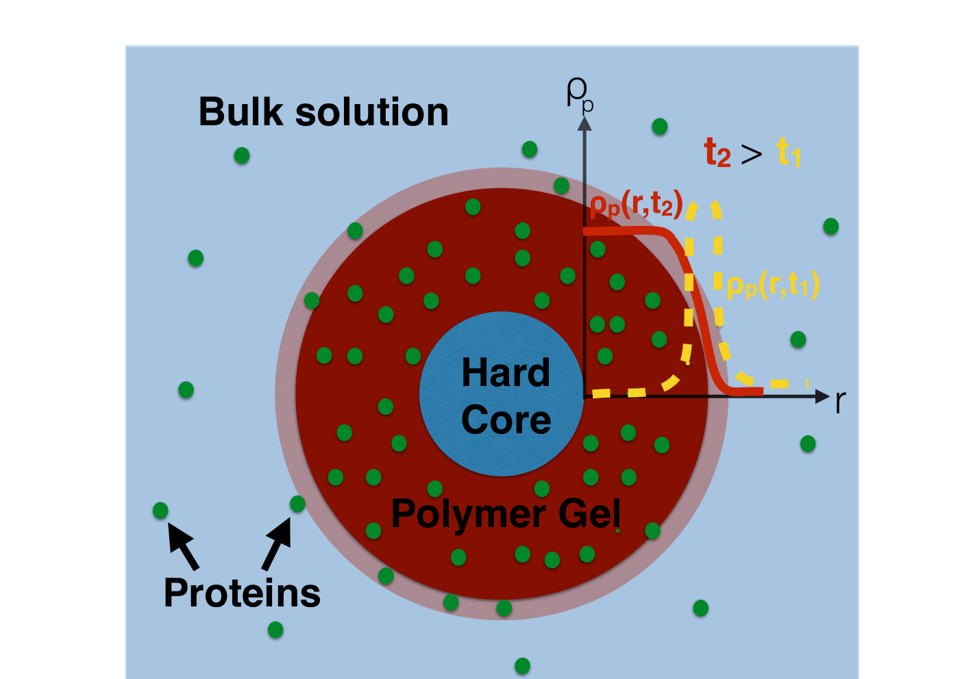
where $R_{core}$ is the radius of the nano particle hard-core (see Fig. 1), and the outer boundary $L$ depends on the nanogel number density $\rho_{np}$, as specified later in Sec. 4. The initial density profile is taken to be a homogeneous density equal to the initial bulk density value $\rho_{p}^{bulk}$, except in the nanogel where it is taken to be zero, corresponding to a possible setup where nanoparticles are inserted in an otherwise equilibrated solution of proteins. This problem can be fully solved analytically by standard Fourier techniques. We will only report here the final form of the solution for clarity, where we also assumed $D_{p}$ to be constant in space

		$\displaystyle\rho_{p}\left(r,t\right)=C_{0}+{1\over r}\sum_{n=1}^{n=\infty}\exp{\left(-\lambda_{n}^{2}D_{p}t\right)}N_{n}^{-1}C_{n}\phi_{n}(r)$		(27)
		$\displaystyle N^{-1}_{\lambda_{n}}=$		(28)
		$\displaystyle{2\over\left[\left(\lambda_{n}^{2}+{1\over R_{core}^{2}}\right)\left(\left(L-R_{core}\right)-{1\over L\left(\lambda_{n}^{2}+{1\over L^{2}}\right)}\right)\right]+{1\over R_{core}}}$
		$\displaystyle C_{n}=\int_{R_{C}}^{L}r^{\prime}\theta\left(r^{\prime}-R_{gel}\right)\phi_{n}(r^{\prime})dr^{\prime}$		(29)
		$\displaystyle\phi_{n}(x)=\lambda_{n}\cos\left(\lambda_{n}r\right)+{1\over R_{core}}\sin\left(\lambda_{n}r\right)$		(30)

where $C_{0}$ is nothing but the average value of the initial density in the domain, i.e.

$\displaystyle C_{0}={3\over 4\pi\left(L^{3}-R_{core}^{3}\right)}\int_{R_{core}}^{L}4\pi r^{2}\rho_{p}^{bulk}\theta\left(r-R_{gel}\right)dr,$

(31)

and $\lambda_{n}$ is given by the solution of the following transcendental equation

$\displaystyle\tan\left(\lambda_{n}\left(L-R_{core}\right)\right)={\lambda_{n}\left(L-R_{core}\right)\over 1+\lambda_{n}^{2}LR_{core}},$

(32)

where $n$ labels the infinitely many solution for this equation.
The solution to this problem is quite instructive, and we discuss some of its main features here. First of all, a timescale $\tau_{D}={\left(L-R_{core}\right)^{2}\over D_{p}}$ appears. Note that this timescale does not contain any reference to $R_{Gel}$, i.e. the radius of the nanogel. Moreover, at the typical densities encountered in experiments, one has that $L>>R_{core}$, hence the only relevant timescale is controlled by the nanogel average distance $L$, itself a function of the nanogel density, $L\approx\rho_{np}^{-1/3}$ (see Sec. 4). This would mean that the adsorption kinetics for micron- or nano-sized gels, if measured at the same number density, will be the same within this model. If experiments instead are made at constant packing fraction $\rho V_{nanogel}$, which scales as $R_{gel}^{3}$, than the loading dynamics will be many orders of magnitude faster for nanogels. This can partially rationalise the very different timescales observed in the experiments for these two systems ^{38, 5}. If we plug into the definition of $\tau_{D}$ the values of $L$ for the experiments we are trying to describe ¹⁴ (see Sec. 4), which is about $10^{3}$ nm, and the diffusion coefficient of lysozime in water, which is of order $D_{p}\approx 0.1\mathrm{nm}^{2}/\mathrm{ns}$ ⁵, by truncating Eq. 30 to the first few terms in $n$, we obtain an estimate of $t_{1/2}\approx 2\cdot 10^{-3}\tau_{D}=2\cdot 10^{-2}$ ms.
The reason for which diffusion is here much faster than for the Debye case is that we properly took into account the full density evolution, which has initially a strong density gradient -hence associated flux- at the nanogel/solution boundary, whereas in the Debye case we simply used the steady state value of the flux to calculate the loading. Regardless, we will see later in Sec. 4 how neither the timescales nor the density profile obtained from the solution of the ideal diffusion equation correspond to what is observed for our DDFT model, warranting that ideal diffusion equations should be taken very carefully when used as an interpretative model for experimental data, even from a qualitative point of view.

Before discussing the dynamics of our system, it is of interest to look at the final equilibrium solution, in order to highlight the role played by the various term in determining the final equilibrium density profile $\rho_{p}^{e}\left(\mathbf{x}\right)$ . This can be obtained by looking for the density profile for which $J(\mathbf{x})=0$, or, equivalently, minimising the free-energy functional (Eq. 6) under the constraint of a fixed number of proteins, leading to:

		$\displaystyle\rho_{p}^{e}\left(\mathbf{x}\right)=$
		$\displaystyle\rho_{0}e^{\left(-\beta\mu^{eq}_{p}\right)}e^{\left[-\beta\left(V^{ext}(\mathbf{x})+\epsilon^{exc}\left(\{\rho^{e}_{p}(\mathbf{x})\}\right)+\rho_{p}^{e}\left(\mathbf{x}\right){\partial\epsilon^{exc}\left(\{\rho^{e}_{p}(\mathbf{x})\}\right)\over\partial\rho_{p}}\right)\right]}.$		(34)

where the quantity $\rho_{0}e^{\left(-\beta\mu^{eq}_{p}\right)}$ is determined by imposing a fixed number of proteins $N_{p}$ in our cell volume for each species in the system, i.e.

$$\int_{R_{core}}^{R_{cell}}4\pi r^{2}\rho_{p}^{e}\left(r\right)dr=N_{p}=V_{cell}\rho_{p}^{bulk}.$$

(35)

where $\rho_{p}^{bulk}$ is the initial bulk concentration of protein $p$ (note that due to mass conservation, the density of proteins in the bulk will diminish due to adsorption onto the nanoparticle). In general, when inter-particle interactions are present and hence the density appears in both sides of Eq. 34, a closed formula for $\rho^{e}_{p}$ cannot be found, and the problem must be solved iteratively starting with a trial density and iterating until self-consistency is achieved.
We report in Fig. 2 the value of the various terms in Eq 8 for the initial (top) and equilibrium (bottom) density distribution.

An important feature to notice in these profiles is the change of some of the thermodynamic forces in their slope at the gel/bulk solution boundary (i.e. R=1), since this is related to the adsorption flux through the equation

$$J_{p}^{i}(t)=-D_{p}(R_{gel})\rho_{p}(R_{gel},t){\partial\beta\mu_{p}^{i}(R_{gel},t)\over\partial r}$$

(36)

where the superscript $i$ labels the specific thermodynamic potential considered (e.g $V^{\mathrm{Don}},V^{\mathrm{Born}},...$). Indeed, this change means that whereas initially all thermodynamic forces drive the system towards absorbing protein, closer to equilibrium only the Born and intrinsic energy term favour adsorption, whereas the ideal and excess terms, as well as the Donnan potential, prevent it. It is the balance between these opposing terms that determines the final equilibrium, and strongly influences the observed dynamics of the system.

We report the full time evolution of the density profile for the system in Fig. 3.

Let us first discuss these profile qualitatively. Three distinct regimes can be observed. At very short timescales ($t<10\mu$s), a density instability is generated at the boundary between the gel and bulk surface, which propagates towards the nanoparticle hard core. This density peak stems from competition between a very strong energy gradient at the gel-bulk boundary which pushes protein towards the gel together with the reduced diffusion coefficient in the gel region, which is about $1/10$ that in the bulk solution, which causes proteins to accumulate at the interface. At intermediate timescales ($t<110\mu$s), the density peak diffuses far enough towards the gel/hardcore boundary, an appreciable concentration of protein builds up in this region, and the density peak becomes more diffuse, eventually reaching a width approximately equal to the gel width. At this point, a step-like density profile is obtained, and at later times the only qualitative change in the density profile is its height, which grows in time until the full equilibrium loading is reached.
A question that naturally arises is whether a similar dynamical behaviour can be reproduced using a simple diffusion model where only the ideal term is retained, but we still account for the space-dependence of the diffusion coefficient to make a fair comparison. This is what many kinetic models of protein adsorption assume either implicitly or explicitly, completely neglecting the role of energy gradients in the system ⁵. Fig. 4 reports for comparison the evolution of the density profile for the same type of protein described in Fig. 3 but described in terms of the ideal diffusion equation, where the diffusion coefficient has been taken to have the same spatial dependency as for the DDFT model to allow for proper comparison:

It is evident that the dynamics is not only just quantitatively approximate but also qualitatively very different compared to the one obtained using a more realistic model. Moreover, the timescales are clearly off by more than an order of magnitude, given that the density profile for purely ideal diffusion has almost reached its equilibrium value in half a millisecond, in contrary to the full description where at five milliseconds the density profile is still relatively far from being equilibrated. In principle, one could argue that DDFT models might not reproduce the loading dynamics better than the ideal diffusion equation. To show this is not the case, we report for both models in Fig. 5 the time dependence of the loading $\Theta(t)=N(t)/N(\infty)$ (where $N(t)$ is the number of adsorbed proteins, obtained by simply integrating the density over the whole gel volume) and compare it to that extrapolated from fitting of experimental data, as shown in Ref. ³⁸. In this latter paper, it was shown that an empirical Langmuir fit was able to reproduce, using the same parameters, data at different densities. In order to compare our data with those from experiments, we scaled the experimental value to the same protein density studied here ^** * simulations of the density for which experimental data is directly available is not possible since this would require simulating timescales a couple of orders of magnitude higher than those accessible within our model, due to computational limitations.

It should be clear from Fig. 5 that our DDFT description, although still not in complete quantitative agreement with experimental data, is a much better representation then an ideal diffusion model, where the dynamics is off by more than one order of magnitude.

Since an important fact is that ideal diffusion completely neglects the important fluxes due to energy gradient in the systems, it is illuminating to look at how much these contribute to protein loading, as shown in Fig. 6, where we plot the ideal and excess protein flux at the gel-solution boundary (the sum of which, by integration over time, gives the loading). As observed in Fig. 6, the ideal flux in both models are similar. However, the real flux is the sum of the ideal and excess flux, the latter being zero in an ideal diffusion model. In this regard, we notice how the excess flux is always at least comparable if not dominant w.r.t the ideal one, with the result that not taking it into account leads to a wrong estimate of the loading.
In our model, the excess flux is always positive, hence it leads to a higher number of adsorbed proteins per unit time in the DDFT scenario. This is not in contrast with ideal diffusion models relaxing to equilibrium much faster than the more realistic DDFT description because the equilibrium number of proteins calculated within an ideal model is orders of magnitudes smaller than that from DFT. In fact, underestimation of the equilibrium amount of protein is possibly the largest source of error in using the ideal diffusion equation to model protein adsorption ⁵, since it can only predict a final flat equilibrium profile where the density is constant throughout the system. However, as expected from simple thermodynamics arguments, a non-homogeneous density must appear whenever any type of gel/protein interaction is present. Hence, care should be taken when using ideal diffusion models to analyse experimental data. For example, in Ref. ⁵ Li et al. found that in order to obtain the correct timescales, they had to assume the presence of trapping binding sites that reduce the mobility of the proteins, effectively inducing a diffusion constant about 2 to 3 orders of magnitudes lower than that expected for similar polymer/protein systems. Such a small value is probably an artefact arising from not including any electrostatic driving force in their description, since in our DDFT model we were able to obtain the correct timescale without assuming such a surprisingly small diffusion coefficient. The importance of electrostatics is pointed out by the fact that, in the same experiments, they found that the number of expected binding sites (which determines the effective diffusion coefficient) is strongly dependent on pH, varying by a factor of 20 in the pH range $[3-7]$ ⁵.

Given that we observe both qualitative and semi-quantitative agreement with experiments, we can confidently use the current model to investigate the sorption kinetics for different scenarios, and try to rationalise the observed trends. In particular, we assess here how the dynamics changes as a function of four important parameters characterising our system, i.e. protein valence, nanoparticles and protein’s concentration and intrinsic adsorption energy. We do this by looking at both the unnormalised and normalised amount of adsorbed proteins, $N(t)$ and $\Theta(t)$. As previously done in Sec. 3 we will take as an informative quantity to measure the speed of the kinetics the time to achieve half the equilibrium loading, $t_{1/2}$, which we report in Table 1. The standard values for the parameters in the following simulations are $\beta\Delta G^{ads}=-1$, $\rho_{p}=2.02\cdot 10^{-4}$ M, $\rho_{np}=3.36\cdot 10^{-9}$ M and $Z=1$, and in each set of simulations one of this quantity is varied keeping the other fixed. The parameters describing the nanoparticle, such as its radius or that of the polymer gel coating it, are the same as those for the Lysozyme model. Fig. 7,8 and Table 1 summarise our results:

The observed trends in Fig. 7 and Fig. 8 can be rationalised in terms of two balancing mechanisms. On the one side, higher driving forces, for example a lower $\Delta G^{ads}$ or higher protein concentration should lead to a faster kinetics, given that higher fluxes are expected. The same should happen for lower nanoparticle concentrations, for which the counter flux, introduced via the boundary conditions that account for proteins being adsorbed by neighbouring particles, is reduced. This is indeed the case, because at any one time the amount of adsorbed proteins is an increasing function of these driving forces, as can be observed from the unnormalised adsorption profiles of Fig. 8. On the other side, however, higher driving forces (with the only exception of the protein’s valence, which deserve a separate discussion later) also lead to a higher number of adsorbed proteins at equilibrium.
Clearly, if both the equilibrium number of proteins adsorbed and the average fluxes were linearly increasing functions of these driving forces, $\Theta(t)$ for different parameter values, i.e. Fig. 7 should collapse onto a single curve. Instead, a very different behaviour is observed. In fact, it turns out that the increase in the total flux when higher driving forces are present is not always enough to compensate for the higher value of proteins that must be adsorbed to reach equilibrium, hence the loading dynamics can be slower. For example, loading as a function of increasing (in modulus) adsorption energy becomes slower, whereas it is faster if we simply increase the initial bulk concentration of proteins, $\rho_{p}^{bulk}$, despite in both ways we are increasing both the adsorption fluxes and $N(\infty)$. However, although $N(\infty)$ as a function of $\rho_{p}^{bulk}$ grows more rapidly than for $\Delta G^{ads}$, its associated flux increases even faster and the overall loading dynamics is actually faster and not slower for this latter case. As this example shows, the fact that both fluxes and equilibrium adsorption are highly non-linear functions of the control parameters implies that predictions based on simple arguments can be highly misleading, and one really has to solve the full equation of motion to rationalise these behaviours. To make an even simpler example, let us just point out that for ideal diffusion the loading dynamics is not even a function of the bulk protein concentration, $\rho_{p}^{bulk}$.

An even stronger manifestation of non-linear behaviour can be observed in our system for the case of $\Theta(t)$ as a function of protein’s charge $Z$. In this case, $t_{1/2}$ has a maximum for $Z=3$ and then decreases, a type of non-monotonic behaviour which would be difficult to predict without a full DDFT modelling. This maximum again arises since the total amount of adsorbed proteins at equilibrium $N(\infty)$ as a function of their charge rapidly saturates (see Fig. 8 and compare the $Z=3$ and $Z=5$), whereas the thermodynamic force for adsorption does not (at least until charge inversion of the loaded gel occurs). Saturation is expected because of two competing effects. On the one hand, when a protein of unlike charge absorbs the system decreases its energy by an amount $\mid ZV^{\mathrm{Don}}\mid$. However, $V^{\mathrm{Don}}$ is itself a function of the adsorbed charge, and becomes lower the higher the number of proteins in the gel. Hence, a maximum amount of adsorbed particles exists, when the adsorption of one more protein would effectively increase the total electrostatic potential felt in such a way that no-more energy is gained. Given the form of $V^{\mathrm{Don}}$ ( Eq. 15 ), this is expected to happen earlier for proteins of higher charge.
We would like to stress the fact that it would be difficult to rationalise these effect looking purely at the loading dynamics $\Theta(t)$ and not at the “raw” quantity $N(t)$, since the latter typically shows a different behaviour. In particular, terms as “fast” or “slow” dynamics should be used based on one or the other quantity in order to avoid confusion, especially when comparing different systems, like for example nanoparticles of different size. In this regard, we notice that many analysis of experimental results are often based on $\Theta(t)$ alone, although in principle such techniques have access to the raw quantity as well.

What additional insights do these simulations offer regarding protein adsorption adsorption on nanogels? One thing to notice is that the parameters’ range scanned in this systematic study covers typical values observed for protein-nanogels system, and the timescales observed should thus be indicative of those expected in realistic scenarios. In this regard, we would like to highlight the fact that here protein adsorption occurs on timescales of a few milliseconds. Whereas this will depend on the exact concentration of both nanoparticles and proteins, it is nonetheless many orders of magnitude faster than that observed in typical anti-fouling applications such as PEG-coated surfaces ⁴, or for bare nanoparticles ^{6, 7}. Hence, it is reasonable to assume that in this system the protein’s corona always reaches equilibrium with the local environment. This fact can have important repercussions on large-scale models for farmacokinetics, since it would justify modelling the nanoparticles behaviour in the human body assuming the protein corona (i.e. the nanoparticles ”biological identity” ^{3, 41}) rapidly adapts to the changes in pH, protein and salt concentration found in different tissues (given that transport between different parts of the body of these nanoparticles by either diffusion or convection through the blood-stream occurs on timescales a few orders of magnitude higher). This is clearly not the same behaviour one can assume to describe, for example, protein induced degradation in a biomedical implant, since the protein adsorption kinetics in this case will necessarily play a much more important role given the long times required to achieve equilibrium.
These conclusions might be challenged when considering the case of competitive protein adsorption when multiple types are present, which will be studied in a future publication.

References

- 1 K. Nakanishi, T. Sakiyama and K. Imamura, Journal of Bioscience and Bioengineering, 2001, 91, 233–244.
- 2 S. D. D. Tenzer, J. Kuharev, A. Musyanovych, V. Fetz, R. Hecht, F. Schlenk, D. Fischer, K. Kiouptsi, C. Reinhardt, K. Landfester, H. Schild, M. Maskos, S. K. Knauer and R. H. Stauber, Nature Nanotechnology, 2013, 8, 772–781.
- 3 M. Monopoli, A. Christoffer, A. Salvati and K. Dawson, Nature Nanotechnology, 2012, 7, 779–786.
- 4 Q. Wei, T. Becherer, S. Angioletti-Uberti, J. Dzubiella, C. Wischke, A. Neffe, A. Lendlein, M. Ballauff and R. Haag, Angewandte Chemie International Edition, 2014.
- 5 Y. Li, Z. Zhang, H. P. van Leeuwen, M. A. Cohen Stuart, W. Norde and J. M. Kleijn, Soft Matter, 2011, 7, 10377–10385.
- 6 D. Dell’Orco, M. Lundqvist, C. Oslakovic, T. Cedervall and S. Linse, PLoS ONE, 2010, 5, e10949.
- 7 F. Darabi Sahneh, C. Scoglio and J. Riviere, PLoS ONE, 2013, 8, e64690.
- 8 F. Fang and I. Szleifer, Biophysical Journal, 2001, 80, 2568 – 2589.
- 9 F. Fang and I. Szleifer, The Journal of Chemical Physics, 2003, 119, 1053–1065.
- 10 M. A. Carignano and I. Szleifer, Colloids and Surfaces B: Biointerfaces, 2000, 18, 169 – 182.
- 11 F. Fang, J. Satulovsky and I. Szleifer, Biophysical Journal, 2005, 89, 1516 – 1533.
- 12 J. B. Schwartz, A. P. Simonelli and W. I. Higuchi, Journal of Pharmaceutical Sciences, 1968, 57, 274–277.
- 13 Y. Samuelov, M. Donbrow and M. Friedman, Journal of Pharmaceutical Sciences, 1979, 68, 325–329.
- 14 C. Yigit, N. Welsch, M. Ballauff and J. Dzubiella, Langmuir, 2012, 28, 14373–14385.
- 15 U. M. B. Marconi and P. Tarazona, The Journal of Chemical Physics, 1999, 110, 8032–8044.
- 16 M. Rex and H. Löwen, Phys. Rev. Lett., 2008, 101, 148302.
- 17 M. Rex, H. H. Wensink and H. Löwen, Phys. Rev. E, 2007, 76, 021403.
- 18 R. Wittkowski and H. Löwen, Molecular Physics, 2011, 109, 2935–2943.
- 19 B. D. Goddard, A. Nold, N. Savva, P. Yatsyshin and S. Kalliadasis, Journal of Physics: Condensed Matter, 2013, 25, 035101.
- 20 J. Wu and Z. Li, Annual Review of Physical Chemistry, 2007, 58, 85–112.
- 21 R. Evans, Advances in Physics, 1979, 28, 143–200.
- 22 J. P. Hansen and I. MacDonald, Theory of Simple Liquids, Academic Press, 4th edn., 2013.
- 23 M. Schmidt and J. M. Brader, The Journal of Chemical Physics, 2013, 138, 214101–214109.
- 24 J. M. Brader and M. Schmidt, The Journal of Chemical Physics, 2013, 139, 104108–104114.
- 25 C. P. Royall, J. Dzubiella, M. Schmidt and A. van Blaaderen, Phys. Rev. Lett., 2007, 98, 188304.
- 26 A. Malijevský and A. J. Archer, The Journal of Chemical Physics, 2013, 139, 144901–144913.
- 27 M. Krüger and J. M. Brader, EPL (Europhysics Letters), 2011, 96, 68006.
- 28 F. Penna, J. Dzubiella and P. Tarazona, Phys. Rev. E, 2003, 68, 061407.
- 29 A. J. Archer, M. J. Robbins and U. Thiele, Phys. Rev. E, 2010, 81, 021602.
- 30 F. Penna and P. Tarazona, The Journal of Chemical Physics, 2003, 119, 1766–1776.
- 31 L. Almenar and M. Rauscher, Journal of Physics: Condensed Matter, 2011, 23, 184115.
- 32 J. Dzubiella and C. N. Likos, Journal of Physics: Condensed Matter, 2003, 15, L147.
- 33 W. A. Curtin and N. W. Ashcroft, Phys. Rev. A, 1985, 32, 2909–2919.
- 34 M. B. Jackson, Molecular and Cellular Biophysics, 1st edn., 2006.
- 35 C. Mattisson, P. Roger, B. Jönsson, A. Axelsson and G. Zacchi, Journal of Chromatography B: Biomedical Sciences and Applications, 2000, 743, 151 – 167.
- 36 Y. Li, Z. Zhang, H. P. van Leeuwen, M. A. Cohen Stuart, W. Norde and J. M. Kleijn, Soft Matter, 2011, 7, 10377–10385.
- 37 D. I. Devore and G. S. Manning, Biophys. Chem., 1978, 2, 42.
- 38 N. Welsch, J. Dzubiella, A. Graebert and M. Ballauff, Soft Matter, 2012, 8, 12043–12052.
- 39 O. Annunziata, D. Buzatu and J. G. Albright, Langmuir, 2005, 21, 12085–12089.
- 40 D. Brune and S. Kim, Proc. Natl. Acad. Sci. USA, 1993, 90, 3835–3839.
- 41 M. Lundqvist, J. Stigler, G. Elia, I. Lynch, T. Cedervall and K. A. Dawson, Proceedings of the National Academy of Sciences, 2008, 105, 14265–14270.
- 42 L. Vroman and A. Adams, Surface Science, 1969, 16, 438 – 446.
- 43 S. L. Hirsh, D. R. McKenzie, N. J. Nosworthy, J. A. Denman, O. U. Sezerman and M. M. M. Bilek, Colloids and Surfaces B: Biointerfaces, 2013, 103, 395 – 404.