Mobile linkers on DNA-coated colloids: valency without patches
Abstract
Colloids coated with single-stranded DNA (ssDNA) can bind selectively to other colloids coated with complementary ssDNA. The fact that DNA-coated colloids (DNACCs) can bind to specific partners opens the prospect of making colloidal ‘molecules’. However, in order to design DNACC-based molecules, we must be able to control the valency of the colloids, i.e. the number of partners to which a given DNACC can bind. One obvious, but not very simple approach is to decorate the colloidal surface with patches of single-stranded DNA that selectively bind those on other colloids. Here we propose a design principle that exploits many-body effects to control the valency of otherwise isotropic colloids. Using a combination of theory and simulation, we show that we can tune the valency of colloids coated with mobile ssDNA, simply by tuning the non-specific repulsion between the particles. Our simulations show that the resulting effective interactions lead to low-valency colloids self-assembling in peculiar open structures, very different from those observed in DNACCs with immobile DNA linkers.
During the past two decades there has been substantial progress in the functionalization of
colloidal particles with various ligand-receptor pairs such as complementary single-stranded DNA (ssDNA) sequences [1, 2].
ssDNA grafting makes it possible to control the specificity of inter-particle
interactions [3, 4, 5]: two grafted ssDNA sequences bearing
complementary Watson-Crick sequences can hybridise to form a
double-stranded DNA (dsDNA) bridge between two particles, thus generating an effective attraction.
In contrast, particles coated with non-complementary sequences do not attract.
Exploiting this mechanism to tune colloidal interactions, DNA functionalisation has enabled the design
of a variety of self-assembling nano-particle lattices [6, 7, 8],
thus opening the way towards new functional materials [9].
However, at present our ability to design arbitrary structures is limited by the fact that it is not straightforward to control the coordination number (i.e. valency) in such colloidal structures.
For instance, low-valency colloids can self-assemble into open structures [10] that do not form if inter-particle interactions are pairwise additive and isotropic.
On the atomic scale, carbon can form diamonds, where atoms are 4-coordinated, because carbon atoms have a well-defined electronic valency. In contrast,
noble-gases interact through (nearly) pairwise additive interactions and only form dense structures, such as fcc and bcc.
If we wish colloidal particles to self-assemble into a diamond lattice, we need to control their valency.
Colloidal diamond lattices are intensively
studied because
such crystals would facilitate production of
photonics band gap materials [11, 12]. However, their direct self-assembly is currently hampered
by the lack of simple ways to control colloidal valency.
Considerable progress has been made in the (multi-step) synthesis of colloids with a well-defined valency encoded through the
careful positioning of ssDNA linkers in patches at specific positions
.
Wang et al[13] have shown that it is possible to produce colloids with patches in precise locations; DNA can be grafted selectively onto these patches.
In this Letter, we present calculations that indicate that it should be possible
to enforce the valency of colloidal particles without “statically” encoding
it in their structure. Instead, many-body effects naturally arising in
DNACCs with mobile linkers can be exploited to this purpose. Moreover we show
that valency control can be tuned by changing the grafting density of inert strands, temperature
or salt concentration.
As an illustration we consider a binary system of colloids,
and (see Fig. 1), covered with mobile and DNA strands.
Each strand terminates in a short sequence of complementary ssDNA, and .
Such colloids have been previously synthesised in various ways, as described in Refs. [14, 15].
When the suspension is cooled below a specific (sequence-dependent) temperature, the
ssDNA will hybridise with its complement, forming bonds between the DNACCs.
Reliable techniques exist [16, 17] to predict the strength of attraction between
and colloids as a function of temperature.
Same-type colloids (i.e. or pairs) repel each other
due to the steric repulsion between non-binding ssDNA.
The interactions between colloids coated with mobile ssDNA are not pairwise additive.
Consider two DNACCs, and , brought to a distance where hybridisation is possible.
These two colloids will experience an attraction with a strength that increases with the number of bonds.
If a second colloid of type (here, ) is inserted in the system at
the same distance from colloid as colloid (Fig. 1), any of the mobile DNA strands on can now hybridise with either or .
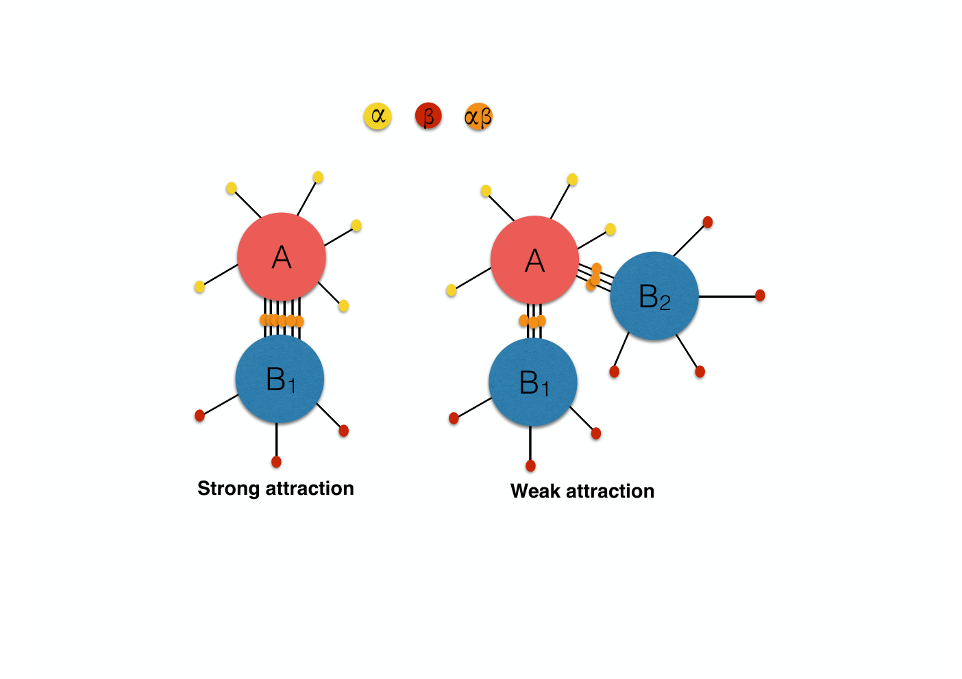
The symmetry of the problem requires that on average the same number of bonds will form
between and and
and . Since the strength of the effective inter-particle interaction
is an increasing function of the number of bonds
and given that there is a finite number of strands to form bonds,
the presence of a third colloid lowers the effective attraction between two particles.
This many-body effect is at the basis of the mechanism controlling valency in this class of colloids.
However, and this is our key point, the decrease of the binding strength per bond with the number of neighbours
is not enough to control the colloidal valency, as
the maximum number of neighbours is determined by
the total cluster interaction energy: each new bonding partner makes inter-particle interactions weaker
but adds one more interacting pair. In the absence of non-specific repulsions, the highest coordination numbers are most favourable.
However, if we add non-specific repulsions to the colloidal interactions, we can tune the optimal coordination number.
To make our argument quantitative, we calculate the effective interactions in different clusters.
To this end, we need an expression for the interaction free-energy of a cluster where the colloids positions are fixed at
arbitrarypositions. We then relax the fixed-positions constraint and perform
Monte Carlo (MC) simulations where the colloids positions are allowed to
achieve their equilibrium distribution.
Our expression for the effective interaction between DNACCs is based on the mean-field approach developed in
Refs. [16, 17], and used to describe a variety of systems [18, 19, 20, 21].
As shown in ref. [17], this approach yields quantitative agreement with MC
simulations.
Ref. [17] showed that the attractive part of the
effective interaction free-energy induced by a system of ligand-receptor pairs (e.g.
complementary DNA-strands) with bonding energies
(where and label two specific binding partners) is
approximated remarkably well by the following expression:
| (1) |
where is the probability that linker is unbound and is the probability that linkers and form a bond. These quantities are given by solving the following set of equations:
| (2) | ||||
| (3) |
where is the free energy for the formation of a single bond between the pair. The latter can be rewritten in a more insightful form as [16, 22]:
| (4) |
where is the hybridisation free-energy for two DNA strands in solution.
depends only on DNA sequence and is a function of temperature and salt concentration [23, 24].
, an explicit function of the grafting
points , is the configurational cost associated with the bond formation, and has been previously quantified
both for single and double-stranded DNA [16, 23].
For the case of mobile DNA, all strands with the same recognition sequence that reside on
the same colloid are equivalent since they cannot be distinguished by their grafting position.
In this case, the correct procedure is to replace by its average over all possible grafting points.
Hence, the effective, single-bond strength between types and residing on colloids and , respectively, will
be given by
| (5) |
where the average is taken keeping the centre of colloid at fixed and is the area of the colloid. In Eq. 5 we use greek subscripts to label a strand type (rather than specific strands as in Eqs. 3,2). We follow this convention from now on. Using Eqs. 2, 3 to replace in Eq. 1, and considering that strands of the same type are equivalent and hence have the same value for , we obtain:
| (6) |
and
| (7) |
Eq. 6 is a system of equations, one for each possible non-equivalent strand in the system:
its solution is an explicit function of all colloidal positions .
Hence, if two strands cannot bind because they are grafted on distant colloids, and the sum over in
Eq. 6 effectively runs only on strand types on neighbouring colloids.
Eqns. 6, 7 are key results of this paper. They allow to calculate
the bond-mediated binding energy for any two generic objects interacting via mobile linkers.
We show in the SI that for mobile linkers these formulas become exact in the limit of large numbers of linkers.
Let us first consider clusters made of colloid of type surrounded by colloids of type at equivalent positions ( by symmetry only two types of strands are present, and ) for which Eqs. 6,7 become:
| (8) |
and
| (9) |
Eq. 9 (closed-form solution in SI) gives only the contribution due to bonds formation between ligands, and is purely attractive. For typical DNACCs realisations, other terms due to van-der-Waals forces or electrostatic interactions are negligible at the binding distance between colloids of a few nanometers imposed by the DNA length [22]. Hence, their effect can be safely disregarded. However, other terms due for example to the presence of inert DNA-strands or other polymers can still be relevant. These polymers act as steric stabilisers via excluded volume interactions, giving a repulsive energy of general form:
| (10) |
where is the partition function counting all accessible states of the
polymers given the positions of the colloids
and is the same partition function when the colloids are at infinite separation.
As for , the contribution due to Eq. 11 can be calculated exactly for selected
polymeric architectures or otherwise computed with MC simulations [16].
To illustrate the effect of non-specific repulsion, first consider the case that between two colloids has a constant value
. The total energy of a cluster then has an additional term
. Added to Eq. 9, we obtain a closed analytical
expression for the free-energy of a cluster .
If we divide by the number of neighbours, we obtain the total energy per
bonding pair (Eq. 18-22 in the SI).
Fig. 2 confirms that is always an increasing function of the number of colloids, hence attraction in an pair becomes weaker by increasing the number of neighbours. However, it is that controls the valency distribution function. Without a local minimum in , the latter peaks at the highest possible coordination number (i.e. 12 for equal-sized spheres). A minimum in appears only if a finite repulsion is present, in which case the valency distribution peaks at a lower value dependent on (dashed and continuous curves in the inset), suggesting a viable route to tune DNACCs’ valency.
In practice, the repulsive energy at the equilibrium distance can be controlled
by coating colloids with inert DNA strands or other polymers that are somewhat longer than
the ‘sticky’ DNA strands [19].
Based on these results, we expect that in a realistic system of DNACCs
with mobile linkers one can control the average valency by varying temperature or salt concentration.
We also expect, based on Eqs. 5,11, that the specific value of
at which a particular valency is stabilised will depend on the grafting
density and the size of the colloids, since both these parameters enter in our equations.
To demonstrate this, we performed MC simulations of an equimolar mixture of colloids
that can move freely.
was calculated by using Eq. 11 and considering the case of mobile strands
(details of its calculation are reported in the SI). We stress that our outcomes are insensitive
to the precise choice of .
We take two specific realisation of the system, differing in the presence or absence of long inert strands.
Each colloid is modelled as a hard sphere with a radius nm on which rigid, double stranded DNA of length
nm terminating with a short single-stranded DNA sequence are grafted (as in the plots for Fig. 2).
In the system with inert strands, additional strands of dsDNA of length nm are added.
Since , the persistence length of ds-DNA, linkers can be described as rigid rods [22],
for which both the contribution to the repulsive energy as well for mobile linkers
can be calculated analytically given the colloids’ positions (see the SI).
This model for the DNA-construct corresponds to the experimental realisation described in [25, 26, 27, 22].
In each run, MC sweeps per particles are made, starting with 100 colloids in random positions at
packing fraction 0.05 and at various values of .
Each trial move consists of a random displacement , and the total free-energy recalculated
using Eqs. 6,7 under periodic boundary conditions.
The analysis was performed every 100 sweeps per particle, and the valency distribution function ( in the inset of Fig. 2)
was calculated using the maximum bonding distance, i.e. for rigid rods.
Results are presented in Fig. 3, for the case with (left) and without (right) inert strands,
corresponding to and , respectively.


These results support the conclusions based on the simpler analytical model
derived for the quenched-cluster system: repulsion plays an important role in stabilising low-valency structures.
In particular, higher repulsion shifts the average valency to lower values.
As predicted by our simplified model, the valency probability distribution can be tuned
by changing , i.e. temperature
or salt concentration.
The observed valency distribution for colloids without inert strands is relatively broad,
which can mainly be attributed to finite size effects in our system.
Although we did not calculate the equilibrium phase diagram for this system, all observed structures assemble
quickly and spontaneously from a random configuration and remain stable, suggesting
at least metastability.
Without inert strands a compact and well ordered crystal forms, whereas the open structures observed in
their presence lack long-range order. This is not necessarily required to achieve interesting functional properties:
low valency was shown to be enough to obtain structures with a proper, 3-dimensional photonic band-gap [28].
Finally, we note that Feng et al [15] have reported the experimental observation of low-valency
structures of deformable, micron-sized oil droplets coated with mobile DNA. In this system, the repulsion mechanism is
droplet deformation. As we have not applied our theory to this case, we cannot yet conclude whether droplet deformation
alone can limit valency.
To conclude, in this this paper we have studied the collective behaviour of a suspensions of binary isotropic colloids functionalised by mobile linkers. We showed how the interaction parameters can be tuned to induce the self–assembly of aggregates exhibiting a desired number of neighbours. Our model indicates that such a valency control can be achieved by changing the non-specific repulsion between colloids and is a function of temperature and salt concentration. We also derive an explicit formula for the bonding-energy of a system of mobile linkers, provide the set of self-consistent equations needed to calculate it, and show how they can be used to drive an MC algorithm to efficiently sample the DNA-mediated free-energy. Hence beyond motivating experimental work towards the design of low valency structures, we provide tools to model other systems interacting via reversible mobile binders: an obvious example is the interaction between lipid vesicles [29], or functionalised particles with cell membranes, whose interaction strongly depends on ligand-receptor bonds formation [30].
I Acknowledgments
S.A-U acknowledges support from the Alexander von Humboldt Foundation via a Postdoctoral Fellowship. This work was supported by the European Research Council Advanced Grant 227758, the Wolfson Merit Award 2007/R3 of the Royal Society of London and the Engineering and Physical Sciences Research Council Programme Grant EP/I001352/1. P.V. has been supported by a Marie Curie International Incoming Fellowship of the European Community’s Seventh Framework Programme under contract number PIIF-GA-2011-300045, and by a Tizard Junior Research Fellowship from Churchill College.
References
- [1] C. A. Mirkin, R. C. Letsinger, R. C. Mucic, and J. J. Storhoff, Nature 382, 607 (1996).
- [2] A. P. Alivisatos, K. P. Johnsson, X. Peng, T. E. Wilson, C. J. Loweth, M. P. Bruchez, and P. G. Schultz, Nature 382, 609 (1996).
- [3] D. Nykypanchuk, M. M. Maye, D. van der Lelie, and O. Gang, Langmuir 23, 6305 (2007), http://pubs.acs.org/doi/pdf/10.1021/la0637566 .
- [4] P. L. Biancaniello, A. J. Kim, and J. C. Crocker, Phys. Rev. Lett. 94, 058302 (2005).
- [5] A. J. Kim, P. L. Biancaniello, and J. C. Crocker, Langmuir 22, 1991 (2006), http://pubs.acs.org/doi/pdf/10.1021/la0528955 .
- [6] S. Y. Park, A. K. R. Lytton-Jean, B. Lee, S. Weigand, G. C. Schatz, and C. A. Mirkin, Nature Materials 451, 553 (2008).
- [7] D. Nykypanchuk, M. M. Maye, D. van der Lelie, and O. Gang, Nature Materials 451, 549 (2008).
- [8] R. Macfarlane, B. Lee, M. Jones, N. Harris, G. Schatz, and C. A. Mirkin, Science 334, 204 (2011).
- [9] Y. Zhang, L. Fang, K. Yager, D. van der Lelie, and O. Gang, Nature Nanotechnology 8, 865 (2013).
- [10] F. Romano, E. Sanz, and F. Sciortino, The Journal of Chemical Physics 134, 174502 (2011).
- [11] J. D. Joannopoulos, P. R. Villeneuve, and S. Fan, Nature 386, 143 (1997).
- [12] S. Linden, C. Enkrich, M. Wegener, J. Zhou, T. Koschny, and C. M. Soukoulis, Science 306, 1351 (2004), http://www.sciencemag.org/content/306/5700/1351.full.pdf .
- [13] Y. Wang, Y. Wang, D. R., V. N. Manoharan, L. Feng, A. D. Hollingsworth, M. Weck, and D. J. Pine, Nature 491, 51 (2012).
- [14] S. A. J. van der Meulen and M. E. Leunissen, Journal of the American Chemical Society 135, 15129 (2013), http://pubs.acs.org/doi/pdf/10.1021/ja406226b .
- [15] L. Feng, L.-L. Pontani, R. Dreyfus, P. Chaikin, and J. Brujic, Soft Matter 9, 9816 (2013).
- [16] P. Varilly, S. Angioletti-Uberti, B. M. Mognetti, and D. Frenkel, The Journal of Chemical Physics 137, 094108 (2012).
- [17] S. Angioletti-Uberti, P. Varilly, B. M. Mognetti, A. Tkachenko, and D. Frenkel, The Journal of Chemical Physics 138, 021102 (2013).
- [18] B. M. Mognetti, P. Varilly, S. Angioletti-Uberti, F. Martinez-Veracoechea, J. Dobnikar, M. Leunissen, and D. Frenkel, Proceedings of the National Academy of Sciences 109 (2012), doi/10.1073/pnas.1119991109.
- [19] S. Angioletti-Uberti, B. M. Mognetti, and D. Frenkel, Nature Materials 11, 518 (2012).
- [20] F. Martinez Veracoechea, B. M. Mognetti, S. Angioletti-Uberti, P. Varilly, D. Frenkel, and J. Dobnikar, Soft Matter 10, 3463 (2014).
- [21] B. M. Mognetti, M. E. Leunissen, and D. Frenkel, Soft Matter 8, 2213 (2012).
- [22] M. E. Leunissen and D. Frenkel, Journal of Chemical Physics 134, 084702 (2011).
- [23] L. Di Michele, B. M. Mognetti, T. Yanagishima, P. Varilly, Z. Ruff, D. Frenkel, and E. Eiser, Journal of the American Chemical Society 136, 6538 (2014), http://pubs.acs.org/doi/pdf/10.1021/ja500027v .
- [24] J. SantaLucia, Proceedings of the National Academy of Sciences of the United States of America 95, 1460 (1998), http://www.pnas.org/content/95/4/1460.full.pdf+html .
- [25] M. E. Leunissen, R. Dreyfus, F. C. Cheong, D. G. Grier, R. Sha, N. C. Seeman, and P. M. Chaikin, Nature Materials 8, 590 (2009).
- [26] M. E. Leunissen, R. Dreyfus, R. Sha, N. C. Seeman, and P. M. Chaikin, Journal of the American Chemical Society 132, 1903 (2010), pMID: 20095643, http://pubs.acs.org/doi/pdf/10.1021/ja907919j .
- [27] R. Dreyfus, M. E. Leunissen, R. Sha, A. V. Tkachenko, N. C. Seeman, D. J. Pine, and P. M. Chaikin, Phys. Rev. Lett. 102, 048301 (2009).
- [28] K. Edagawa, S. Kanoko, and M. Notomi, Phys. Rev. Lett. 100, 013901 (2008).
- [29] D. Serien, C. Grimm, J. Liebscher, A. Herrmann, and A. Arbuzova, New J. Chem. , (2014).
- [30] G. Bell, Science 200 (1978).
II Supplementary Information
II.1 Accurate approximation for calculating the repulsive free-energy
When colloids are functionalised with grafted polymers under good solvent conditions, polymeric chains act as steric stabilisers via excluded volume interactions. More precisely, they induce a repulsive free-energy between colloids due to the fact that the impenetrable colloids limit the amount of configurations the chains can attain, hence reducing the free-energy of the system. Formally, this can be written as:
| (11) |
where is the partition function counting all accessible states of the
polymers given the positions of all other colloids in the system (see note 11
1
For non spherical colloids, their orientation should also be considered)
and is for isolated colloids (see Fig. 4(a) for reference).
We take the polymers to be ideal, and hence simply counts the number of available geometric states, which are all considered to have exactly the same energy and hence
the same weight, i.e. the system is athermal.
In our model, the polymer is a stiff, double-stranded (ds) DNA of length terminating with a small, point-like recognition sequence.
Since we assume ( being the persistence length of dsDNA), we can describe it as a rigid rod whose grafting point
can move on the surface. As we are about to show, in this case a very accurate analytic approximation
exists for Eq. 11, which becomes better and better in the limit , being the radius of the colloid
on which the strand is grafted.


Let us first introduce a quantity, , defined as the probability that the end point of our rod (i.e that not grafted to the surface) is at a position (see Fig. 4(b) for reference). is given by the following expression:
| (12) |
where the Dirac delta function takes care of fixing the rod length and the Heaviside step function makes sure that the rod does not penetrate the colloid on which is coated. The integral in Eq. 12 can be calculated giving the following result:
| (13) |
which, for small , can be further approximated as
| (14) |
i.e. is uniform. Our first approximation will be to take this uniform value for . Let us now make a second approximation, whose validity also increases in the limit (where now labels a colloid among the neighbours on which the polymer is grafted). We will count as allowed states for our rod all those for which its end-point is not inside a neighbouring colloid (see Fig. 4 for reference). Note that within this approximation we are (wrongly) counting as allowed configurations those where the rod overlaps a neighbour for a fraction which does not include the end point (see 4(c)). Given that we take a flat probability distribution, the number of these states is simply proportional to the overlap volume between a sphere of radius and that of a sphere of radius , given by:
| (15) |
Since the total number of states available for a grafted rod when no other colloids are present is proportional to the volume accessible to its end-point , the following equation holds:
| (16) |
hence, considering that rods behave as ideal (i.e. they do not interact with each other), we find the following final expression for the repulsive free-energy induced by mobile rods grafted on a surface of a colloid due to the presence of its neighbours with positions :
| (17) |
To appreciate the difference between the analytic approximation and a numerically accurate Monte Carlo estimation of , we report in Fig. 5 the repulsive free-energy between two colloids calculated in both ways for two colloids coated with 70 strands of either length or , as in our simulations.
Whereas the difference is negligible for the short rods, it starts to become relevant for the longer ones. However, we observe that a simple
rescaling procedure can be used to get accurate results, i.e. one can take and the data reproduces
the accurate numerical results for all colloids distances (for the longer strands , note that its
value depends on the specific ratio).
This is equivalent to saying that, by using the analytical estimate for , we are effectively simulating a system whose grafting density is
about 1.5 times larger than the real one.
For the sake of computational efficiency and reproducibility, in our simulations we always use the analytic approximation. Hence, if
one intends to experimentally replicate the system, a higher coverage should be used (for the value of in our model, this is still well in
the range of values used in experiments).
As for , a similar approach can be taken in our system to calculate (Eq. 4 in the main text), i.e. the entropic configurational penalty to form a bond between two DNA strands. In our case, is the configurational free-energy penalty to confine the end of two grafted rods at the same location (or, better, within a bonding volume [21, 16]). This is given by [16]:
| (18) |
where is the standard concentration, M, is the phase space allowed for two strands and grafted at colloid and respectively and bound to each other, and the phase space allowed for two grafted but unbound strands, i.e. calculated previously. Using exactly arguments and approximations previously used to calculate , the following holds:
| (19) |
II.2 Large number of linkers limit of the bonding free-energy in the presence of mobile linkers:
In this section we show that the set of self-consistent equations developed for DNA coated colloids (Eqs. 6 in the manuscript), and the free energy used (Eq. 7 in the manuscript) are exact when the number of DNA-strands (linkers, from now on) becomes large. This is shown by using a saddle–point approximation.
The DNA partition function for a set of colloids at fixed positions is given by
| (20) |
where the factors have been defined in Manuscript Eq. 5 (here we omit the dependence of on the colloids’ position). counts all the possible combinations of DNA–DNA hybridisation resulting in bridges between particle and particle with (Fig. 6). In the definition of (Eq. 20) the first product is taken on all the type of linkers while the second on all possible pairs of types. Linkers are of different types if they are either grafted on different colloids or have a different recognition sequences. The partition function is then defined as in Eq. 20 taking the sum on all the possible sets of pairs consistent with a total number of strands in the system weighted with the total hybridisation free energy (as given by Manuscript Eq. 5).
The derivation of is shown in Fig. 6 for the case in which different types correspond to different particles. The generalisation to the case in which more than one family of DNA is present on a single colloid is straightforward. Starting from a configuration with no bonds formed (in which for all and ), the number of ways of making bridges between particle and particle is given by (see Fig. 6)
In the previous expression we have accounted for the indistinguishability of the bridges and is the total number of linkers present on the particle . At the next step we count the number of possible combinations resulting in bridges between particle and finding
resulting in a total number of configurations (see Fig. 6)
In the previous expression we recognise the factorisation of Eq. 20 in term of type terms (first three terms) and type–type terms (last two term). Recursively adding the missing bridges (e.g. see Fig. 6 for ) it is easy to see that we obtain an expression for that remains consistent with Eq. 20.
Using a Stirling approximation we can write the partition function (Eq. 20) as
| (21) | |||||
In the limit in which (with fixed) the number of linkers distribution functions peak around the saddle point solution defined by
| (22) |
The free energy of the system () is then given by
| (23) |
| (24) |
Now we show that Eq. 24 is equivalent of Eq. 6 in the main text. This can be done identifying the probability that a tethers of type to be free as
where is the number of tethers of type unbound. Using we can write the tether balance as
| (25) |
Using Eq. 24 in Eq. 25 we obtain the same set of equations found in the manuscript
| (26) |
with .
Using the previous equation in 21 we find
| (30) |
which again is equivalent to Eq. 7 in the main text.
In Ref. [17], Equations 1-3 of the main text, from which the final self-consistent equations and the free-energy of the system of mobile linkers are obtained here, were derived assuming that the conditional probability for a linker to be unbound given that another one was unbound was independent from the latter. Since for the case of mobile linkers we obtain the same functional equations considering an exact partition function, this means that in this latter case the approximation becomes exact in the limit where a large number of linkers is present.
II.3 An analytical expression for
Eq. 8 in the main text can be solved to give:
| (31) |
Combining this solution to Eq. 9 in the main text, the following formula arises for the bonding part of the free-energy of a cluster of an colloid coated with linkers surrounded by neighbours, each coated with linkers, in equivalent positions (linkers and are complementary and can form a bond with average energy , see main text for details).
| (32) | ||||
| (33) | ||||
| (34) | ||||
| (35) | ||||
| (36) |