Statistical estimation of jump rates for a specific class of Piecewise Deterministic Markov Processes.

N. Krell ^†^†thanks: Université de Rennes 1, Institut de Recherche mathématique de Rennes, CNRS-UMR 6625, Campus de Beaulieu. Bâtiment 22, 35042 Rennes Cedex, France. email: nathalie.krell@univ-rennes1.fr

Abstract

We consider the class of Piecewise Deterministic Markov Processes (PDMP), whose state space is $\mathbb{R}_{+}^{*}$ , that possess an increasing deterministic motion and that shrink deterministically when they jump. Well known examples for this class of processes are Transmission Control Protocol (TCP) window size process and the processes modeling the size of a "marked" Escherichia coli cell. Having observed the PDMP until its $n$ th jump, we construct a nonparametric estimator of the jump rate $\lambda$ . Our main result is that for $D$ a compact subset of $\mathbb{R}_{+}^{*}$ , if $\lambda$ is in the Hölder space ${\mathcal{H}}^{s}({\mathcal{D}})$ , the squared-loss error of the estimator is asymptotically close to the rate of $n^{-s/(2s+1)}$ . Simulations illustrate the behavior of our estimator.

Keywords: Piecewise Deterministic Markov processes, Nonparametric estimation, jump rate estimation, ergodicity of Markov chains.
Mathematical Subject Classification: 62M05, 62G05, 62G20, 60J25.

1 Introduction

The Piecewise deterministic Markov processes were first introduced in the literature by Davis ([18] and [19]), they form a family of càdlàg Markov processes involving a deterministic motion punctuated by random jumps. We refer to the paper [7] and its references for an overview of PDMPs. Let us detail the special case of PDMPs that will be considered in this paper. The motion of the PDMP $(X(t))_{t\geq 0}$ depends on three local characteristics, namely the jump rate $\lambda$ , the flow $\phi$ and a deterministic increasing function $f$ which governs the location of the process at the jump time (in the general case it depends on a Markov kernel $Q$ ). The process starts from $x$ and follows the flow $\phi(x,t)$ until the first jump time $T_{1}$ which occurs spontaneously in a Poisson-like fashion with rate $\lambda(\phi(x,t))$ . The location of the process at the jump time $T_{1}$ , denoted by $Z_{1}=X(T_{1})$ , is equal to $f(X(T_{1}^{-}))$ , with $f$ a function such that $0\leq f(y)\leq\kappa y$ with $0<\kappa<1$ . The motion restarts from this new point $Z_{1}$ as before. This fully describes a piecewise continuous trajectory for $\{X(t)\}$ with jump times $\{T_{k}\}$ and post jump locations $\{Z_{k}\}$ , and which evolves according to the flow $\phi$ between two jumps.

This paper analyzes a special case of both Piecewise Deterministic Markov process (PDMPs) and growth-fragmentation model.

The fisrt known example for this class of processes is the TCP window size process (see [11], [16], [21], [22] and [23]). The TCP protocol is one of the main data transmission protocols of the Internet. It has been designed to adapt to the various traffic conditions of the actual network. For a connection, the maximum number of packets that can be sent at each round is given by a variable $W$ , called the congestion window size. If all the $W$ packets are successfully transmitted, then $W$ is increased by 1, otherwise it is multiplied by $\delta\in(0,1)$ (detection of a congestion). As shown in [21] a correct scaling of this process leads to a continuous time Markov process, called general TCP window size process.

The second example is the processes modeling the size of a "marked" Escherichia coli cell (see [20] and [24]). If by following the evolution of Escherichia coli bacterium, we chose at random a bacteria, and follow his growth, and at his division, we choose randomly, and independently of the process, to follow one of his daughter and on so one. We call the bacteria follow at each time, the "marked" bacteria. The size of the "marked" bacteria is a PDMP. More precisely between the jumps, the bacteria grows exponentially with a growth rate which we will refer to later as the instantaneous growth rate. The division rate of such process is denoted by $B(\cdot)$ and at each jump its size is divided by two.

In both cases the value of the process is divided in a deterministically way at each jump.

The purpose of this article is to perform non-parametric estimation of the jump rate based on a single observation of the process over a long time interval.

The assumptions made in this paper ensure that the Markov process which gives the size after each jump of the PDMP is ergodic. The ergodic theorem was already known for some cases of PDMPs and for some one-dimensional jump-diffusions. In [17] Cloez studies a process which is more general than the one considered in this paper. More precisely, his process evolves like a diffusion which satisfies a stochastic differential equation between the jumps, but he requires that $\lambda$ be bounded below. This paper does not make such assumption. In addition, the well known ergodicity properties of TCP, due to J.-M. Bardet et al. [11], provide quantitative estimates for the exponential convergence to equilibrium, in terms of the total variation and Wasserstein distances. However, such results cannot be used in the present framework as we need a uniform upper bound for the speed of convergence to the invariant measure over a certain class of functions in order to prove the statistical result.

Our approach is based on the methods used by Doumic et al. [20], which were applied to analyse a special case of PDMPs dealing with “marked” bacteria size evolution. The analytical results of this paper can be generalized to more general PDMPs, for example to TCP. In [20] the authors do not merely study the "marked" bacterium which is selected at each division uniformly and independently, but the evolution of all bacteria involved. A dependence structure results when, for example, a bacteria divides and gives birth to two new bacterium of equal size. In a general case, the instantaneous growth rate (constant for a given bacteria) would depend on the bacteria itself. Consequently, the size of the bacterium is no longer a Markov process. However, on the other hand, the size of the process and the instantaneous growth rate, together form a Markov process. The present paper contains the case of a "marked" bacterium, in its simple case, where the instantaneous growth rate is the same for all bacteria.

This article has two main features that may be useful for future studies. First, it can be used as a tool to verify the PDMP jump rate proposed in the existing literature, for example $\lambda(x)=x$ in the TCP case. Secondly, it can suggest an estimator for some special cases, such as for Escherichia coli bacteria, where the jump rate is not known.

In [9] Azaïs et al. give an estimator of the conditional distribution of the inter-jump times for a PDMP, which is uniformly consistent when only one observation of the process within a long time is available. They deal with PDMPs which jump when they hit the boundary (this case is not considered in our paper). Their method relies on a generalization of Aalen’s multiplicative intensity model [1, 2, 3]. But they only prove the uniform consistency of their estimator. They also have to assume that the process $(X(t))_{t\geq 0}$ evolves in a bounded space. Here we do not make this assumption. As a consequence the tools of their paper and of the present one are different. To the best of my knowledge, [9] is the only work investigating the nonparametric estimation of the conditional distribution of the inter-arrival times for PDMPs. This paper relies on [8] in which the authors focus on the non parametric estimation of the jump rate and the cumulative rate for a class of non homogeneous marked renewal processes. The case where the post-jump locations of the PDMP do not depend on inter-arrival times was considered in [8].

We refer to [9] for an overview of the statistical methods related to this kind of process, as well as to [2, 3, 1] for statistical inference related to the multiplicative intensity model. The book of Andersen et al. [4] gives a comprehensive account of estimation for jump rates which depend both on time and spatial variable.

As far as I know, the only other paper dealing with general PDMP is the work of Azaïs [6], where the author focuses on a non parametric recursive estimator for the transition kernel of the PDMP.

Other works dealing with specific cases of PDMP can been seen as ruin probability, for example, as found in the references of [5]. In addition, the PDMP modeling the quantity of a given food contaminant in the body has been studied in [15, 13, 14], assuming that the inter-intake times are i.i.d.. In this paper we do not make this assumption.

The paper of Azaïs and Genadot [10] consider a growth-fragmentation model where $\lambda$ is constant and the Markov kernel $Q$ is absolutely continuous with respect to the Lebesgue measure. The case considered is totally different from the present one.

The paper is organized as follows. In section 2 we introduce the class of PDMPs, that will be studied, and we give an explicit construction of the PDMP. Section 3 concerns the statistical estimation of the jump rate. We first define the observation scheme and the class of functions for the 3 parameters of the PDMP concerned, and the assumptions used (in Subsection 3.2). In subsection 3.3, some ergodicity results are stated uniformly over the class of functions previously defined. We explicitly construct an estimator $\widehat{\lambda}_{n}$ of $\lambda$ . In subsection 3.5 an upper bound for the squared-error loss is given in the main Theorem 1. In 3.6, we illustrate our result with simulations of a TCP process which could not been seen as a "marked" bacteria process, amongst others.

Finally, section 4 is reserved for the proofs. In subsection 4.1 we prove the ergodicity result of Subsection 3.3. Subsection 4.2 presents the intermediate results needed in 4.3 to prove the major results given in Subsection 3.5.

2 PDMP

In general a PDMP is defined by its local characteristics, namely, the jump rate $\lambda$ , the flow $\phi$ and the transition measure $Q$ according to which the location of the process is chosen at the jump time. In this article, we consider a specific class of PDMP which includes the control of congestion TCP/IP used in communication networks (V. Dumas and al [21], V. Guillemin and al. [23]), for which the transition measure $Q$ is a Dirac mass function, which means that when the process jumps, the size after the jump is a deterministic function of its size before. More precisely,

Assumption 1.

•

The flow $\phi:\mathbb{R}^{+}\times\mathbb{R}^{+}\rightarrow\mathbb{R}^{+}$ is a one-parameter group of homeomorphisms: $\phi$ is $\mathcal{C}^{1}$ , $\phi(.,t)$ is an homeomorphism for each $t\in\mathbb{R}^{+}$ , satisfying the semigroup property: $\phi(.,t+s)=\phi(\phi(.,s),t)$ and $\phi_{x}(.):=\phi(x,.)$ is an $\mathcal{C}^{1}$ -diffeormorphism.
•

The jump rate $\lambda:\mathbb{R}^{+}\rightarrow\mathbb{R}_{+}$ is assumed to be a measurable function satisfying

$\forall x\in\mathbb{R}^{+},\;\;\exists\>\varepsilon>0\>\;\text{such that}\>\;\int_{0}^{\epsilon}\lambda(\phi(x,s))ds<\infty.$
•

$f:\mathbb{R}^{+}\rightarrow\mathbb{R}^{+}$ is an increasing $\mathcal{C}^{1}$ -diffeomorphism and $Q(u,\{y\})={\mathchoice{\rm 1\mskip-4.0mul}{\rm 1\mskip-4.0mul}{\rm 1\mskip-4.5mul}{\rm 1\mskip-5.0mul}}_{\{f(u)=y\}}$ .

Given these three characteristics, it can be shown ([19], pages 62-66), that there exists a filtered probability space $(\Omega,\mathcal{F},\{\mathcal{F}_{t}\},\{\mathbb{P}_{x}\})$ such that the motion of the process $\{X(t)\}$ starting from a point $x\in\mathbb{R}^{+}$ may be constructed as follows. Consider a random variable $T_{1}$ such that

\mathbb{P}_{x}(T_{1}>t)=e^{-\Lambda(x,t)},

(1)

where for $x\in\mathbb{R}^{+}$ and $t\in\mathbb{R}^{+}$

\Lambda(x,t)=\int_{0}^{t}\lambda(\phi(x,s))ds.

If $T_{1}$ is equal to infinity, then the process $X$ follows the flow, i.e. for $t\in\mathbb{R}_{+}$ , $X(t)=\phi(x,t)$ . Otherwise let

Z_{1}=f(\phi(x,T_{1})).

(2)

The trajectory of $\{X(t)\}$ starting at $x$ , for $t\in[0,T_{1}]$ , is given by

X(t)=\begin{cases}\phi(x,t)&\text{for }t<T_{1},\\ Z_{1}&\text{for }t=T_{1}.\end{cases}

Inductively starting from $X(T_{n})=Z_{n}$ , we now select the next inter-jump time $T_{n+1}-T_{n}$ and post-jump location $X(T_{n+1})=Z_{n+1}$ in a similar way.

This construction properly defines a strong Markov process $\{X(t)\}$ with jump times $\{T_{k}\}_{k\in\mathbb{N}}$ (where $T_{0}=0$ ). A very natural Markov chain is linked to $\{X(t)\}$ , namely the jump chain $(Z_{n})_{n\in\mathbb{N}}$ .

$\{X(t)\}$ is a Markov process with infinitesimal generator $G$ :

Gh(y)=\phi_{x}^{{}^{\prime}}(y)h^{{}^{\prime}}(y)+\lambda(y)\big(h(f(y))-h(y)\big)

(3)

for $h:\mathbb{R}^{+}\rightarrow\mathbb{R}$ a bounded measurable functional.

Thanks to (1), we get that

\mathbb{P}(T_{1}\in dt|Z_{0}=x)=\lambda(\phi_{x}(t))e^{-\int_{0}^{t}\lambda(\phi_{x}(s))ds}dt.

Using (2), the monotonicity of $f\circ\phi_{x}$ and a simple change of variables, we get the transition probability of the Markov chain $(Z_{n})_{n\in\mathbb{N}}$ :

\mathbb{P}(Z_{1}\in dy|Z_{0}=x)=\lambda(f^{-1}(y))e^{-\int_{f(x)}^{y}\lambda(f^{-1}(s))g_{x}(s)ds}g_{x}(y){\mathchoice{\rm 1\mskip-4.0mul}{\rm 1\mskip-4.0mul}{\rm 1\mskip-4.5mul}{\rm 1\mskip-5.0mul}}_{\{y\geq f(x)\}}dy,

(4)

where

g_{x}(y)=\left[(f\circ\phi_{x})^{{}^{\prime}}\left((f\circ\phi_{x})^{-1}(y)\right)\right]^{-1}

and $\phi_{x}(.):=\phi(x,.)$ .

3 Statistical estimation of the jump rate

3.1 The observation scheme

Statistical inference is based on the observation scheme:

(X(t),t\leq T_{n})

and asymptotics are considered when the number of jumps of the process, $n$ , goes to infinity.

Actually the simpler observation scheme:

(X(T_{i}),1\leq i\leq n)=(Z_{i},1\leq i\leq n)

is sufficient.

3.2 Class of functions

We want to bound from above the squared-loss error of our estimator over compact intervals ${\mathcal{D}}$ of $\mathbb{R}_{+}^{*}$ . We need to specify the local smoothness properties of $\lambda$ over ${\mathcal{D}}$ , together with general properties that ensure that the empirical measurements of the PDMP converge toward the invariant probability with an appropriate speed of convergence. So we have to impose technical assumptions on $\lambda$ in particular near the origin and infinity.

Definition 1.

For $b>0$ , a vector of positive constants $\mathfrak{c}=(r,\kappa,l,L,a)$ , and two positive functions $m:[0,\infty)\rightarrow(0,\infty)$ and $M:[0,\infty)\rightarrow(0,\infty)$ such that for all $x\in[0,\infty):$ $M(x)\geq m(x)>0$ , we introduce the class ${\mathcal{F}}(\mathfrak{c},m,M)$ of triples of continuous functions $\lambda:[0,\infty)\rightarrow[0,\infty)$ , $f:\mathbb{R}^{+}\rightarrow\mathbb{R}^{+}$ and $\phi:\mathbb{R}^{+}\times\mathbb{R}^{+}\rightarrow\mathbb{R}^{+}$ such that

\int_{0}^{f(r)}M(s)\lambda(f^{-1}(s))ds\leq L,

(5)

\int_{f(r)}^{\infty}m(s)\lambda(f^{-1}(s))ds=\infty,

(6)

\int_{f(r)}^{r}M(s)\lambda(f^{-1}(s))ds\geq l,

(7)

\lambda(x)\geq\frac{a(f(x))^{b}}{m(f(x))}\>\;\forall x\geq r,

(8)

\forall x>0,\>\;\>0<f(x)\leq\kappa x,

(9)

\forall y>0,\>\;\>\forall x\geq 0,\>\;\>m(y)\leq g_{x}(y)\leq M(y),

(10)

where

g_{x}(y)=\left[(f\circ\phi_{x})^{{}^{\prime}}\left((f\circ\phi_{x})^{-1}(y)\right)\right]^{-1}

and $\phi_{x}(\cdot)=\phi(x,\cdot)$ .

We notice that $f(0)=0$ .

Typically an interesting case would be $f(x)=\kappa x$ with $\kappa\in(0,1)$ and then (10) would simply be

M^{-1}(y)\leq\kappa\phi_{x}^{{}^{\prime}}(\phi_{x}^{-1}(y/\kappa))\leq m^{-1}(y).

This seems quite reasonable because, in view of the definition of the infinitesimal generator of the PDMP defined in (3), we would like $\phi_{x}^{{}^{\prime}}(\cdot)$ not to be identically zero.

Also the cases where $\phi_{x}(t)=xe^{\alpha t}$ or $\phi_{x}(t)=x+t$ satisfy (10) over ${\mathcal{D}}$ .

Define

\delta(\mathfrak{c},f):=\frac{1}{1-\kappa^{b+1}}\exp\big(-(1-\kappa^{b+1})\tfrac{am}{b+1}(f(r))^{b+1}\big).

The last assumption that we will need is:

Assumption 2.

\exists b>0:(\kappa^{b+1}-1)\frac{am}{b+1}(f(r))^{b+1}<\log(1-\kappa^{b+1}),

(11)

so that we have $\delta(\mathfrak{c},f)<1$

Fix a vector of positive constants $\mathfrak{c}=(r,\kappa,l,L,a)$ , a constant $b$ and a function $f$ .

3.3 Geometric ergodicity of the discrete model

Let $x\in\mathbb{R}^{+}$ . Introduce the transition kernel

\mathcal{P}_{\lambda}(x,dx^{\prime})=\mathbb{P}\big(Z_{n}\in dx^{\prime}\big|\,Z_{n-1}=x\big)

of the size of the process at the $n$ th jump time, given the size of the process at the $(n-1)$ th jump time. From (4), we infer that $\mathbb{P}(Z_{1}\in dy|Z_{0}=x)$ is equal to

\lambda(f^{-1}(y))e^{-\int_{f(x)}^{y}\lambda(f^{-1}(s))g_{x}(s)ds}g_{x}(y){\mathchoice{\rm 1\mskip-4.0mul}{\rm 1\mskip-4.0mul}{\rm 1\mskip-4.5mul}{\rm 1\mskip-5.0mul}}_{\{y\geq f(x)\}}dy.

Thus we obtain an explicit formula for

\mathcal{P}_{\lambda}(x,dy)=\mathcal{P}_{\lambda}(x,y)dy

with

\mathcal{P}_{\lambda}(x,y)=\lambda(f^{-1}(y))e^{-\int_{f(x)}^{y}\lambda(f^{-1}(s))g_{x}(s)ds}g_{x}(y){\mathchoice{\rm 1\mskip-4.0mul}{\rm 1\mskip-4.0mul}{\rm 1\mskip-4.5mul}{\rm 1\mskip-5.0mul}}_{\{y\geq f(x)\}}.

(12)

Denote the left action of positive measures $\mu(dx)$ on $\mathbb{R}^{+}$ for the transition kernel $\mathcal{P}_{\lambda}$ by

\mu\mathcal{P}_{\lambda}(dy)=\int_{\mathbb{R}^{+}}\mu(dx)\mathcal{P}_{\lambda}(x,dy)

and the right action of a function $\psi$ on $\mathbb{R}$ for the transition $\mathcal{P}_{\lambda}$ by

\mathcal{P}_{\lambda}\psi(x)=\int_{\mathbb{R}^{+}}\psi(y)\mathcal{P}_{\lambda}(x,dy)

We now give the geometric ergodic theorem that we will need for the statistical part. We need an uniformity on the class of functions ${\mathcal{F}}(\mathfrak{c},m,M)$ defined in subsection 3.2.

We introduce the Lyapunov function

{\mathbb{V}}(x)=\exp\left(\frac{a}{b+1}(f(x))^{b+1}\right)\;\;\text{for}\;\;x\in\mathbb{R}^{+}.

(13)

The function ${\mathbb{V}}$ controls the rate of the geometric ergodicity of the chain with transition $\mathcal{P}_{\lambda}$ and appears in the proof of Proposition 1.

Proposition 1.

Under Assumption 1, for every $\lambda$ such that $(\lambda,f,\phi)\in{\mathcal{F}}(\mathfrak{c},m,M)$ there exists a unique invariant probability measure of the form $\nu_{\lambda}(dx)=\nu_{\lambda}(x)dx$ on $\mathbb{R}^{+}$ . Moreover there exist $0<\gamma<1$ , a constant $R$ and a function $\mathbb{V}:\mathbb{R}^{+}\rightarrow[1,\infty)$ such that

\sup_{\lambda\in{\mathcal{F}}(\mathfrak{c},m,M)}\sup_{|\psi|\leq V}\big|\mathcal{P}_{\lambda}^{k}\psi(x)-\int_{\mathbb{R}^{+}}\psi(z)\nu_{\lambda}(z)dz\big|\leq R{\mathbb{V}}(x)\gamma^{k}

(14)

for every $x\in\mathbb{R}^{+}$ , $k\geq 0$ , where the supremum is taken over all functions $\psi:\mathbb{R}^{+}\rightarrow\mathbb{R}$ satisfying $|\psi(x)|\leq{\mathbb{V}}(x)$ for all $x\in\mathbb{R}^{+}$ . The function ${\mathbb{V}}$ is $\nu_{\lambda}$ -integrable for every $\lambda$ such that $(\lambda,f,\phi)\in{\mathcal{F}}(\mathfrak{c},m,M)$ .

For all $y\in\mathbb{R}^{+}$ we have the relation:

\lambda(y)\mathbb{E}_{\nu_{\lambda}}(g_{Z_{0}}(f(y)){\mathchoice{\rm 1\mskip-4.0mul}{\rm 1\mskip-4.0mul}{\rm 1\mskip-4.5mul}{\rm 1\mskip-5.0mul}}_{\{f(Z_{0})\leq f(y)\}}{\mathchoice{\rm 1\mskip-4.0mul}{\rm 1\mskip-4.0mul}{\rm 1\mskip-4.5mul}{\rm 1\mskip-5.0mul}}_{\{Z_{1}\geq f(y)\}})=\nu_{\lambda}(f(y)).

(15)

3.4 Construction of a nonparametric estimator

By formula (15),

\lambda(y)=\frac{\nu_{\lambda}(f(y))}{\mathbb{E}_{\nu_{\lambda}}(g_{Z_{0}}(f(y)){\mathchoice{\rm 1\mskip-4.0mul}{\rm 1\mskip-4.0mul}{\rm 1\mskip-4.5mul}{\rm 1\mskip-5.0mul}}_{\{f(Z_{0})\leq f(y)\}}{\mathchoice{\rm 1\mskip-4.0mul}{\rm 1\mskip-4.0mul}{\rm 1\mskip-4.5mul}{\rm 1\mskip-5.0mul}}_{\{Z_{1}\geq f(y)\}})},

provided the denominator is positive. This representation suggests an estimation procedure, replacing the marginal density $\nu_{\lambda}(f(y))$ and the expectation in the denominator by their empirical counterparts. To that end, pick a kernel function

K:\mathbb{R}\rightarrow[0,\infty),\;\;\int_{\mathbb{R}}K(y)dy=1,

and set $K_{h}(y)=h^{-1}K\big(h^{-1}y\big)$ for $y\in\mathbb{R}$ and $h>0$ . Our estimator is defined by

\displaystyle\widehat{\lambda}_{n}(y)=\frac{n^{-1}\sum_{k=1}^{n}K_{h_{n}}(Z_{k}-f(y))}{n^{-1}\sum_{k=1}^{n}g_{Z_{k-1}}(f(y)){\mathchoice{\rm 1\mskip-4.0mul}{\rm 1\mskip-4.0mul}{\rm 1\mskip-4.5mul}{\rm 1\mskip-5.0mul}}_{\{Z_{k}\geq f(y),\,f(y)\geq f(Z_{k-1})\}}\vee\varpi_{n}}.

(16)

where $\varpi_{n}>0$ is a threshold that ensures that the estimator is well defined in all cases and $x\vee y=\max\{x,y\}$ . Thus $(\widehat{\lambda}_{n}(y),y\in{\mathcal{D}})$ is specified by the choice of the kernel $K$ , the bandwidth $h_{n}>0$ and the threshold $\varpi_{n}>0$ .

Assumption 3.

The function $K$ has compact support, and for some integer $n_{0}\geq 1$ , we have $\int_{\mathbb{R}}x^{k}K(x)dx={\bf 1}_{\{k=0\}}\;\;\text{for}\;\;0\leq k\leq n_{0}.$

3.5 Rate of convergence

We are now ready to state our main result. For $s>0$ , with $s=\lfloor s\rfloor+\{s\}$ , $0<\{s\}\leq 1$ and $\lfloor s\rfloor$ an integer, introduce the Hölder space ${\mathcal{H}}^{s}({\mathcal{D}})$ of functions $f:{\mathcal{D}}\rightarrow\mathbb{R}$ possessing a derivative of order $\lfloor s\rfloor$ that satisfies

|f^{\lfloor s\rfloor}(y)-f^{\lfloor s\rfloor}(x)|\leq c(f)|x-y|^{\{s\}}.

(17)

The minimal constant $c(f)$ such that (17) holds defines a semi-norm $|f|_{{\mathcal{H}}^{s}(\mathcal{D})}$ . We equip the space ${\mathcal{H}}^{s}(\mathcal{D})$ with the norm

\|f\|_{{\mathcal{H}}^{s}(\mathcal{D})}=\|f\|_{L^{\infty}({\mathcal{D}})}+|f|_{{\mathcal{H}}^{s}({\mathcal{D}})}

and the associated Hölder balls

{\mathcal{H}}^{s}({\mathcal{D}},M_{1})=\{\lambda:\;\|\lambda\|_{{\mathcal{H}}^{s}({\mathcal{D}})}\leq M_{1}\},\;M_{1}>0.

Theorem 1.

Work under Assumption 1 and Assumption 2. Specify $\widehat{\lambda}_{n}$ with a kernel $K$ satisfying Assumption 3 for some $n_{0}>0$ and

h_{n}=c_{0}n^{-1/(2s+1)},\;\;\varpi_{n}\,\>\;\text{such that}\>\;\lim_{n\rightarrow\infty}\varpi_{n}=0

For every $M_{1}>0$ and $M_{2}>0$ , there exist $c_{0}=c_{0}(\mathfrak{c},M_{1},M_{2})$ and $d(\mathfrak{c})\geq 0$ such that for every $0<s<n_{0}$ and every compact interval ${\mathcal{D}}\subset(d(\mathfrak{c}),\infty)$ such that $\inf{\mathcal{D}}\geq f(r)$ , we have

\sup_{\lambda}\mathbb{E}_{\mu}\big[\|\widehat{\lambda}_{n}-\lambda\|_{L^{2}({\mathcal{D}})}^{2}\big]^{1/2}\lesssim\varpi_{n}^{-2}n^{-s/(2s+1)},

where the supremum is taken over

(\lambda,f,\phi)\in{\mathcal{F}}(\mathfrak{c},m,M),\>\;\>\;\lambda\in{\mathcal{H}}^{s}({\mathcal{D}},M_{1}),\>\;\>\;\>\;g_{x}\in{\mathcal{H}}^{s}({\mathcal{D}}),\>\;\>\;\|f\|_{L^{\infty}({\mathcal{D}})}\leq M_{2},\>\;\>\;\text{and}\>\;f^{-1}\in{\mathcal{H}}^{s}({\mathcal{D}})

and $\mathbb{E}_{\mu}[\cdot]$ denotes expectation with respect to any initial distribution $\mu(d\boldsymbol{x})$ for $(Z_{0})$ on $\mathbb{R}^{+}$ such that $\int{\mathbb{V}}(x)^{2}\mu(dx)<\infty$ .

We observe that we recover the result for the marked bacteria of [20]. In this case $\phi(x,t)=xe^{\kappa_{0}t}$ with $\kappa_{0}\in\mathbb{R}^{+*}$ and $f(x)=x/2$ , so that $g_{x}(y)=\frac{1}{\kappa_{0}y}$ . We find the same estimator but the speed of convergence is a little bit better, as $\varpi_{n}$ need not be $\log(n)$ ; rather we only require that $\lim_{n\rightarrow\infty}\varpi_{n}^{-1}=0$ .

3.6 Numerical implementation

The goal of this subsection is to illustrate the asymptotic behaviour of our estimator via numerical experiments. More precisely we first investigate numerical simulations for the TCP.

The TCP window-size process appears as the scaling limit of the transmission rate of a server uploading packets on the Internet according to the algorithm used in the TCP (Transmission Control Protocol) in order to avoid congestion (see [21] for details on this scaling limit). This PDMP takes values in $\mathbb{R}^{+}$ and the jump rate $\lambda$ is the identity function. The function $f$ which represents the proportion of the size kept after the jump is $f(x)=x/2$ . The flow is $\phi(x,t)=x+t$ .

As a consequence the size of the process after the $n$ -th jump $Z_{n}$ , conditional on $Z_{n-1}$ , has the same law as $\sqrt{(1/4)Z_{n-1}^{2}+e_{n}/2}$ , where $(e_{n})_{n\geq 0}$ is a family of i.i.d. random variables with exponential distribution of parameter 1. The variable $e_{n}$ is also independent of $(Z_{i})_{i\leq n-1}$ . As a consequence it is easy to generate the $(Z_{n})_{n\geq 0}$ recursively. A trajectory of such a PDMP is given in Figure 1. These processes satisfy the assumptions required for our Theorem, with $\kappa=1/2$ , $m(\cdot)=1$ , $M(\cdot)=1.1$ , $g_{\cdot}(\cdot)=1/2$ , $r=1$ , $a=1$ , $b=1/2$ , $\varpi_{n}=(\log(n))^{-1}$ , $h_{n}=n^{-1/3}$ and $K(x)=(2\pi)^{1/2}exp(-x^{2}/2)$ . With the Gaussian Kernel, for which $n_{0}=1$ for Assumption 2, we expect a rate of convergence of order $n^{1/3}$ at best.

We display our numerical results as specified above in Figures 1, 2 and 3.

Figure 2 displays the reconstruction of $\lambda$ for different simulated samples, for $n=1000$ , $n=10000$ and $n=100000$ . As expected, the estimation is better for larger $n$ . The estimator performs worse fo small $x$ as these sizes are rarely reached by the TCP process.

In figure 3, we plot the empirical mean error of our estimation procedure on a $\log$ - $\log$ scale. The numerical results agree with the theory.

Refer to caption — Figure 1: Evolution of the TCP process when 10 jumps occur.

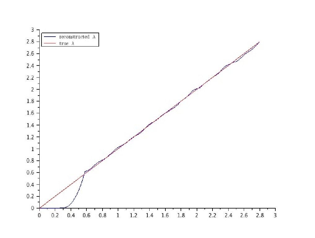
We now consider a bacteria marked case, for which the size of the bacterium are divided by 3 instead of 2 at division. Thus we have $f(x)=x/3$ , $\phi(x,t)=xe^{t}$ and therefore $g_{x}(y)=1/y$ . Let $(e_{i})_{i\in\mathbb{N}^{*}}$ a i.i.d family of exponential law of parameter 1. Conditionally on $Z_{n}=x$ the law of $Z_{n+1}$ is equal in law to $\frac{x}{3}-\frac{1}{3}\log(e_{n+1})$ .

As before Figure 4 displays the reconstruction of $\lambda$ for a simulated sample with $n=100000$ .

4 Proof

4.1 Proof of Proposition 1

We will follow the same idea as in [20]. We prove a minorisation condition, strong aperiodicity and a drift condition for the transition operator $\mathcal{P}_{\lambda}$ in order to use Theorem 1.1 of [12].

Minorisation condition.

Let $\lambda$ be such that $(\lambda,f,\phi)\in{\mathcal{F}}(\mathfrak{c},m,M)$ and set $\mathcal{C}=(0,r)$ where $r$ is specified by $\mathfrak{c}$ . Fix a measurable $A\in\mathcal{F}$ and $x\in\mathcal{C}$ ; thanks to (10), we have

\mathcal{P}_{\lambda}(x,A)\geq\int_{A}\lambda(f^{-1}(y))e^{-\int_{f(x)}^{y}\lambda(f^{-1}(s))M(s)ds}m(y){\mathchoice{\rm 1\mskip-4.0mul}{\rm 1\mskip-4.0mul}{\rm 1\mskip-4.5mul}{\rm 1\mskip-5.0mul}}_{\{y\geq f(x)\}}dy.

We introduce the function $\varphi_{\lambda}$

\varphi_{\lambda}(y):=\lambda(f^{-1}(y))e^{-\int_{0}^{y}\lambda(f^{-1}(s))M(s)ds}m(y)\>\;\>\;\>\>\;\>\;\>\forall y\in\mathbb{R}^{+},

(18)

and the measure $\mu_{\lambda}$

\mu_{\lambda}(dy):=\frac{\varphi_{\lambda}(y)}{c_{\lambda}}{\mathchoice{\rm 1\mskip-4.0mul}{\rm 1\mskip-4.0mul}{\rm 1\mskip-4.5mul}{\rm 1\mskip-5.0mul}}_{\{y>f(r)\}}dy,

where $c_{\lambda}=\int_{f(r)}^{\infty}\varphi_{\lambda}(u)du$ . Thus, we have

\mathcal{P}_{\lambda}(x,A)\geq\mu_{\lambda}(A)c_{\lambda}.

By using (6) and (5), we get that

c_{\lambda}=\int_{f(r)}^{\infty}\varphi_{\lambda}(u)du=\left[\frac{-m(y)e^{-\int_{0}^{y}\lambda(f^{-1}(s))M(s)ds}}{M(y)}\right]_{f(r)}^{\infty}\geq\frac{m(f(r))e^{-L}}{M(f(r))}:=\tilde{\beta}>0.

This shows that the following minorisation condition holds for every $x\in\mathcal{C}$ and $A\in\mathcal{F}$ uniformly in $\lambda$ such that $(\lambda,f,\phi)\in{\mathcal{F}}(\mathfrak{c},m,M)$ :

\mathcal{P}_{\lambda}(x,A)\geq\mu_{\lambda}(A)\tilde{\beta}.

(19)

∎

Strong aperiodicity condition.

We have

	$\displaystyle\mu_{\lambda}(\mathcal{C})\tilde{\beta}$	$\displaystyle=c_{\lambda}^{-1}\tilde{\beta}\int_{f(r)}^{r}\varphi_{\lambda}(y)dy=c_{\lambda}^{-1}\tilde{\beta}\left[\frac{-m(y)e^{-\int_{0}^{y}\lambda(f^{-1}(s))M(s)ds}}{M(y)}\right]_{f(r)}^{r}$
		$\displaystyle=\tilde{\beta}(1-\frac{m(r)M(f(r))}{M(r)m(f(r))}e^{-\int_{f(r)}^{r}\lambda(f^{-1}(s))M(s)ds},)$		(20)

using the computation we just did for $c_{\lambda}$ .

Now we use (7) to get that

\mu_{\lambda}(\mathcal{C})\tilde{\beta}\geq\tilde{\beta}\left(1-\frac{m(r)M(f(r))}{M(r)m(f(r))}e^{-l}\right):=\beta>0.

(21)

∎

Drift condition.

Let $\lambda$ be such that $(\lambda,f,\phi)\in{\mathcal{F}}(\mathfrak{c},m,M)$ and recall that ${\mathbb{V}}:{\mathbb{R}^{+}}\rightarrow[1,\infty)$ , which is defined in (13), is continuously differentiable and satisfies

\lim_{y\rightarrow\infty}{\mathbb{V}}(y)\exp\big(-\tfrac{a}{b+1}y^{b+1}\big)=0.

(22)

For $x\geq r$ , using (10) and integration by parts with the boundary condition (6), we have,

	$\displaystyle\mathcal{P}_{\lambda}{\mathbb{V}}(x)$	$\displaystyle=\int_{f(x)}^{\infty}{\mathbb{V}}(y)\lambda(f^{-1}(y))e^{-\int_{f(x)}^{y}\lambda(f^{-1}(s))g_{x}(s)ds}g_{x}(y)dy$
		$\displaystyle\leq\int_{f(x)}^{\infty}{\mathbb{V}}^{{}^{\prime}}(y)e^{-\int_{f(x)}^{y}\lambda(f^{-1}(s))m(s)ds}dy.$

Thanks to (8), we get that

\begin{array}[]{rcl}\mathcal{P}_{\lambda}{\mathbb{V}}(x)&\leq&\int_{f(x)}^{\infty}{\mathbb{V}}^{{}^{\prime}}(y)e^{-\int_{f(x)}^{y}as^{b}ds}dy\leq e^{a\frac{f(x)^{b+1}}{b+1}}\int_{f(x)}^{\infty}{\mathbb{V}}^{{}^{\prime}}(y)e^{-a\frac{y^{b+1}}{b+1}}dy.\end{array}

Integrating again by parts and using (22), we obtain that

\begin{array}[]{rcl}\mathcal{P}_{\lambda}{\mathbb{V}}(x)&\leq&e^{a\frac{f(x)^{b+1}}{b+1}}\int_{f(x)}^{\infty}{\mathbb{V}}(y)ay^{b}e^{-a\frac{y^{b+1}}{b+1}}dy.\end{array}

Now use the change of variable $z=a\frac{y^{b+1}}{b+1}$ and the definition of ${\mathbb{V}}(x)$ . As (22) is satisfied, we get

\begin{array}[]{rcl}\mathcal{P}_{\lambda}{\mathbb{V}}(x)&\leq&{\mathbb{V}}(x)\int_{a\frac{f(x)^{b+1}}{b+1}}^{\infty}e^{\frac{a}{b+1}\big(f((\frac{z(b+1)}{a})^{1/(b+1)})\big)^{b+1}-z}dz.\end{array}

By using (9), we obtain, for $x\geq r$

\begin{array}[]{rcl}\mathcal{P}_{\lambda}{\mathbb{V}}(x)&\leq&{\mathbb{V}}(x)\int_{a\frac{f(x)^{b+1}}{b+1}}^{\infty}e^{(\kappa^{b+1}-1)z}dz.\end{array}

Therefore,

\mathcal{P}_{\lambda}{\mathbb{V}}(x)\leq{\mathbb{V}}(x)\delta(\mathfrak{c},f),

(23)

with

\delta(\mathfrak{c},f)=\frac{1}{1-\kappa^{b+1}}\exp\big(-(1-\kappa^{b+1})\tfrac{a}{b+1}(f(r))^{b+1}\big),

and we have $\delta(\mathfrak{c},f)<1$ by Assumption 2.

We next need to control $\mathcal{P}_{\lambda}{\mathbb{V}}$ outside $x\in[r,\infty)$ , that is on the small set ${\mathcal{C}}$ . For every $x\in{\mathcal{C}}$ , we have

	$\displaystyle\mathcal{P}_{\lambda}{\mathbb{V}}(x)\leq$	$\displaystyle\Big(\int_{f(x)}^{f(r)}{\mathbb{V}}(y)\lambda(f^{-1}(y))g_{x}(y)dy+\int_{f(r)}^{\infty}{\mathbb{V}}(y)\lambda(f^{-1}(y))e^{-\int_{f(x)}^{y}\lambda(f^{-1}(s))g_{x}(s)ds}g_{x}(y)dy\Big)$
	$\displaystyle\leq$	$\displaystyle\,M\sup_{y\in[0,f(r)]}{\mathbb{V}}(y)L+\delta(\mathfrak{c},f){\mathbb{V}}(r)=:K<\infty,$		(24)

where we used (5), (10), (23) for $x=r$ and the fact that $(\lambda,f,\phi)\in{\mathcal{F}}(\mathfrak{c},m,M)$ . Combining (23) and (24), we conclude that

\mathcal{P}_{\lambda}{\mathbb{V}}(\boldsymbol{x})\leq\delta(\mathfrak{c},f){\mathbb{V}}(\boldsymbol{x}){\mathchoice{\rm 1\mskip-4.0mul}{\rm 1\mskip-4.0mul}{\rm 1\mskip-4.5mul}{\rm 1\mskip-5.0mul}}_{\{\boldsymbol{x}\notin{\mathcal{C}}\}}+K{\mathchoice{\rm 1\mskip-4.0mul}{\rm 1\mskip-4.0mul}{\rm 1\mskip-4.5mul}{\rm 1\mskip-5.0mul}}_{\{\boldsymbol{x}\in{\mathcal{C}}\}}.

(25)

∎

End of the proof of Proposition 1.

By Theorem 1.1 in Baxendale [12] the minorisation condition (19) together with the strong aperiodicity condition (21) and the drift condition (25) imply inequality (14), with $R$ and $\gamma$ that explicitly depend on $\delta(\mathfrak{c},f)$ , $\beta$ , $\tilde{\beta}$ , ${\mathbb{V}}$ and $K$ . By construction, this bound is uniform in $\lambda$ such that $(\lambda,f,\phi)\in{\mathcal{F}}(\mathfrak{c},m,M)$ . More specifically, we have

\gamma<\min\{\max\{\delta(\mathfrak{c},f),\gamma_{\lambda,{\mathbb{V}}}\},1\},

with $\gamma_{\lambda,{\mathbb{V}}}$ the spectral radius of the operator $\mathcal{P}_{\lambda}-1\otimes\nu_{\lambda}$ acting on the Banach space of functions $\psi:R_{+}\rightarrow\mathbb{R}$ such that

\sup\left\{\frac{|\psi(x)|}{\mathbb{V}(x)},\>\;x\in\mathbb{R}_{+}\right\}<\infty.

Therefore, under Assumption (11) we have $\gamma<1$ .

It remains to prove equality (15). As $\mathcal{P}_{\lambda}(x,dy)=\mathcal{P}_{\lambda}(x,y)dy$ and

\nu_{\lambda}\mathcal{P}_{\lambda}=\nu_{\lambda},

we have that $\nu_{\lambda}(dy)=\nu_{\lambda}(y)dy$ and

\begin{array}[]{rcl}\nu_{\lambda}(y)&=&\int_{\mathbb{R}_{+}}\nu_{\lambda}(x)\mathcal{P}_{\lambda}(x,y)dx\\ &=&\int_{\mathbb{R}_{+}}\nu_{\lambda}(x)\lambda(f^{-1}(y))e^{-\int_{f(x)}^{y}\lambda(f^{-1}(s))g_{x}(s)ds}g_{x}(y){\mathchoice{\rm 1\mskip-4.0mul}{\rm 1\mskip-4.0mul}{\rm 1\mskip-4.5mul}{\rm 1\mskip-5.0mul}}_{\{f(x)\leq y\}}dx.\end{array}

Thanks to (6), we get that

e^{-\int_{f(x)}^{y}\lambda(f^{-1}(s))g_{x}(s)ds}=\int_{y}^{\infty}\lambda(f^{-1}(s))g_{x}(s)e^{-\int_{f(x)}^{s}\lambda(f^{-1}(s^{{}^{\prime}}))g_{x}(s^{{}^{\prime}})ds^{{}^{\prime}}}ds.

Therefore,

	$\displaystyle\nu_{\lambda}(y)=$	$\displaystyle\lambda(f^{-1}(y))\int_{\mathbb{R}^{+}}\nu_{\lambda}(x)g_{x}(y){\mathchoice{\rm 1\mskip-4.0mul}{\rm 1\mskip-4.0mul}{\rm 1\mskip-4.5mul}{\rm 1\mskip-5.0mul}}_{\{f(x)\leq y\}}\int_{y}^{\infty}\lambda(f^{-1}(s))g_{x}(s)e^{-\int_{f(x)}^{s}\lambda(f^{-1}(s^{{}^{\prime}}))g_{x}(s^{{}^{\prime}})ds^{{}^{\prime}}}dsdx$
	$\displaystyle=$	$\displaystyle\lambda(f^{-1}(y))\int_{\mathbb{R}^{+}}\nu_{\lambda}(x)g_{x}(y){\mathchoice{\rm 1\mskip-4.0mul}{\rm 1\mskip-4.0mul}{\rm 1\mskip-4.5mul}{\rm 1\mskip-5.0mul}}_{\{f(x)\leq y\}}\int_{y}^{\infty}{\mathchoice{\rm 1\mskip-4.0mul}{\rm 1\mskip-4.0mul}{\rm 1\mskip-4.5mul}{\rm 1\mskip-5.0mul}}_{\{s\geq y\}}\mathcal{P}_{\lambda}(x,s)dsdx$
	$\displaystyle=$	$\displaystyle\lambda(f^{-1}(y))\mathbb{E}_{\nu_{\lambda}}(g_{Z_{0}}(y){\mathchoice{\rm 1\mskip-4.0mul}{\rm 1\mskip-4.0mul}{\rm 1\mskip-4.5mul}{\rm 1\mskip-5.0mul}}_{\{f(Z_{0})\leq y\}}{\mathchoice{\rm 1\mskip-4.0mul}{\rm 1\mskip-4.0mul}{\rm 1\mskip-4.5mul}{\rm 1\mskip-5.0mul}}_{\{Z_{1}\geq y\}}).$

∎

4.2 Rate of convergence for the empirical measure

We now give a few results that we will need for the proof of Theorem 3.2 in the next Subsection. In fact, we decompose the square loss error into a sum of three terms that we will study in the following Propositions.

The notation $\lesssim$ means inequality up to a constant that not depend on $n$ .

Lemma 1.

For any $\mathfrak{c}$ such that Assumptions 2 and 1 are satisfied, there exists a constant $d(\mathfrak{c})\geq 0$ such that for any compact interval ${\mathcal{D}}\subset(d(\mathfrak{c}),\infty)$ , we have

\inf_{\lambda:\>(\lambda,f,\phi)\in{\mathcal{F}}(\mathfrak{c},m,M)}\inf_{x\in{\mathcal{D}}}\varphi_{\lambda}(x)^{-1}\nu_{\lambda}(x)>0,

where $\varphi_{\lambda}(x)$ is defined in (18).

Proof.

Recall that ${\mathbb{V}}(x)=\exp\big(\frac{a}{b+1}(f(x))^{b+1}\big)$ for every $x\in[0,\infty)$ . By Proposition 1 (and, more precisely, equation (14)) we have

\sup_{\lambda:\>(\lambda,f,\phi)\in{\mathcal{F}}(\mathfrak{c},m,M)}\int_{[0,\infty)}{\mathbb{V}}(x)\nu_{\lambda}(x)dx<\infty,

(26)

additionally from (25) in the proof of Proposition 1, we have that $\sup_{\lambda:\>(\lambda,f,\phi)\in{\mathcal{F}}(\mathfrak{c},m,M)}\mathcal{P}_{\lambda}{\mathbb{V}}(x)<\infty$ for every $x\in\mathbb{R}^{+}$ . As a consequence, for every $x\in(0,\infty)$ , we have

\displaystyle\int_{f^{-1}(x)}^{\infty}\nu_{\lambda}(y)dy\;

\displaystyle\leq\exp\big(-\frac{a}{b+1}(f(x))^{b+1}\big)\int_{[0,\infty)}{\mathbb{V}}(y)\nu_{\lambda}(y)dy,

and this bound is uniform in $\lambda$ such that $(\lambda,f,\phi)\in{\mathcal{F}}(\mathfrak{c},m,M)$ by (26). Therefore, for every $x\in(0,\infty)$ , we have

\sup_{\lambda:(\lambda,f,\phi)\in{\mathcal{F}}(\mathfrak{c},m,M)}\int_{f^{-1}(x)}^{\infty}\nu_{\lambda}(y)dy\leq c(\mathfrak{c},f)\exp\big(-\frac{a}{b+1}(f(x))^{b+1}\big),

(27)

for some $c(\mathfrak{c},f)>0$ . Let

d(\mathfrak{c},f)>f^{-1}\big((\frac{b+1}{a}\log(c(\mathfrak{c},f)))^{1/(b+1)}\big).

(28)

By the definition of $\nu_{\lambda}$ and using (10), for every $y\in(0,\infty)$ , we now have

	$\displaystyle\nu_{\lambda}(y)$	$\displaystyle=\int_{0}^{\infty}\nu_{\lambda}(x)\lambda(f^{-1}(y))e^{-\int_{f(x)}^{y}\lambda(f^{-1}(s))g_{x}(s)ds}g_{x}(y){\mathchoice{\rm 1\mskip-4.0mul}{\rm 1\mskip-4.0mul}{\rm 1\mskip-4.5mul}{\rm 1\mskip-5.0mul}}_{\{f(x)\leq y\}}dx$
		$\displaystyle\geq e^{-\int_{0}^{y}\lambda(f^{-1}(s))M(s)ds}\lambda(f^{-1}(y))m(y)\int_{0}^{f^{-1}(y)}\nu_{\lambda}(x)dx$
		$\displaystyle\geq e^{-\int_{0}^{y}\lambda(f^{-1}(s))M(s)ds}\lambda(f^{-1}(y))m(y)\big(1-\int_{f^{-1}(y)}^{\infty}\nu_{\lambda}(x)dx\big)$
		$\displaystyle\geq e^{-\int_{0}^{y}\lambda(f^{-1}(s))M(s)ds}\lambda(f^{-1}(y))m(y)\left(1-c(\mathfrak{c},f)\exp\left(-\frac{a}{b+1}(f(y))^{b+1}\right)\right)$

where we used (27) for the last inequality. By (28), for $y\geq d(\mathfrak{c},f)$ we have

\left(1-c(\mathfrak{c},f)\exp\left(-\frac{a}{b+1}(f(y))^{b+1}\right)\right)>0,

and the conclusion follows readily by the definition of $\varphi_{\lambda}$ . ∎

For every $y\in(0,\infty)$ , define

D(y)=\mathbb{E}_{\nu_{\lambda}}\big[g_{Z_{0}}(f(y)){\mathchoice{\rm 1\mskip-4.0mul}{\rm 1\mskip-4.0mul}{\rm 1\mskip-4.5mul}{\rm 1\mskip-5.0mul}}_{\{Z_{1}\geq f(y),\,f(y)\geq f(Z_{0})\}}\big],

(29)

D_{n}(y)=n^{-1}\sum_{k=1}^{n}g_{Z_{k-1}}(f(y)){\mathchoice{\rm 1\mskip-4.0mul}{\rm 1\mskip-4.0mul}{\rm 1\mskip-4.5mul}{\rm 1\mskip-5.0mul}}_{\{Z_{k}\geq f(y),\,f(y)\geq f(Z_{k-1})\}},

(30)

and

D_{n}(y)_{\varpi_{n}}=\left(n^{-1}\sum_{k=1}^{n}g_{Z_{k-1}}(f(y)){\mathchoice{\rm 1\mskip-4.0mul}{\rm 1\mskip-4.0mul}{\rm 1\mskip-4.5mul}{\rm 1\mskip-5.0mul}}_{\{Z_{k}\geq f(y),\,f(y)\geq f(Z_{k-1})\}}\right)\bigvee\varpi_{n}.

(31)

Proposition 2.

Work under Assumptions 2 and 1. Let $\mu$ be a probability measure on $\mathbb{R}^{+}$ such that $\int_{\mathbb{R}^{+}}{\mathbb{V}}(\boldsymbol{x})^{2}\mu(d\boldsymbol{x})<\infty$ . If $1\geq\varpi_{n}\rightarrow 0$ as $n\rightarrow\infty$ , we have

\sup_{y\in{\mathcal{D}}}\mathbb{E}_{\mu}\big[\big(D_{n}(y)_{\varpi_{n}}-D(y)\big)^{2}\big]\lesssim n^{-1}

(32)

uniformly in $\lambda$ such that

(\lambda,f,\phi)\in{\mathcal{F}}(\mathfrak{c},m,M),\>\;\text{and}\>\;\lambda\in{\mathcal{H}}^{s}({f(\mathcal{D}}),M_{1}),

We first need the following estimate

Lemma 2.

Work under Assumptions 2 and 1. Let $d(\mathfrak{c},f)$ be defined as in Lemma 1. For every compact interval ${\mathcal{D}}\subset(d(\mathfrak{c},f),\infty)$ such that $\inf{\mathcal{D}}\leq f(r)$ , we have

\inf_{\lambda:\>(\lambda,f,\phi)\in{\mathcal{F}}(\mathfrak{c},m,M)\>\;\text{and}\>\;\lambda\in{\mathcal{H}}^{s}(f({\mathcal{D}}),M_{1})}\inf_{y\in{\mathcal{D}}}D(y)>0.

Proof .

By (15) and the definition of $\varphi_{B}$ in (18), we readily have that

D(y)=\frac{\nu_{\lambda}(f(y))}{\lambda(y)}=\frac{\nu_{\lambda}(f(y))}{\varphi_{\lambda}(f(y))}e^{-\int_{0}^{f(y)}\lambda(f^{-1}(s))M(s)ds}m(y).

Since

(\lambda,f,\phi)\in{\mathcal{F}}(\mathfrak{c},m,M)\>\;\text{and}\>\;\lambda\in{\mathcal{H}}^{s}({f(\mathcal{D}}),M_{1}),

by applying (5), we obtain

	$\displaystyle\int_{0}^{f(y)}\lambda(f^{-1}(s))M(s)ds$	$\displaystyle\leq\int_{0}^{\sup{\mathcal{D}}}\lambda(f^{-1}(s))M(s)ds$
		$\displaystyle\leq L+\int_{f(r)}^{\sup\mathcal{D}}\lambda(f^{-1}(s))\sup_{y\in{\mathcal{D}}}\|M(y)\|ds$
		$\displaystyle\leq\left(L+\sup_{y\in{\mathcal{D}}}\|M(y)\|M_{1}\sup{\mathcal{D}}\right)<\infty,$

where we used that $\inf{\mathcal{D}}\leq f(r)$ . It follows that

\inf_{y\in{\mathcal{D}}}\exp\left(-\int_{0}^{f(y)}\lambda(f^{-1}(s))M(s)ds\right)\geq\exp\left(-(L+\sup_{y\in{\mathcal{D}}}|M(y)|M_{1}\sup{\mathcal{D}})\right)>0

and Lemma 2 follows by applying Lemma 1. ∎

Proof of Proposition 2.

Since $D_{n}(y)$ is bounded by $M$ , we have

\big(D_{n}(y)_{\varpi_{n}}-D(y)\big)^{2}\lesssim\big(D_{n}(y)-D(y)\big)^{2}+{\bf 1}_{\{D_{n}(y)<\varpi_{n}\}}.

(33)

Thus, by Lemma 2 we may choose $n$ sufficiently large that

0<\varpi_{n}\leq q=\tfrac{1}{2}\inf_{\lambda:\>(\lambda,f,\phi)\in{\mathcal{F}}(\mathfrak{c},m,M)\>\;\text{and}\>\;\lambda\in{\mathcal{H}}^{s}(f({\mathcal{D}}),M_{1})}\inf_{y\in{\mathcal{D}}}D(y).

Since

\{D_{n}(y)<\varpi_{n}\}\subset\{D_{n}(y)-D(y)<-q\},

by integrating (33), we have that $\mathbb{E}_{\mu}\big[\big(D_{n}(y)_{\varpi_{n}}-D(y)\big)^{2}\big]$ is less than a constant times

\displaystyle\mathbb{E}_{\mu}\big[\big(D_{n}(y)-D(y)\big)^{2}\big]+\mathbb{P}_{\mu}\big(|D_{n}(y)-D(y)|\geq q\big).

By the Bienaymé-Tchebychev inequality, this quantity is less than a constant times

\mathbb{E}_{\mu}\big[\big(D_{n}(y)-D(y)\big)^{2}\big].

Set $G(x,z,y)=g_{x}(f(y)){\mathchoice{\rm 1\mskip-4.0mul}{\rm 1\mskip-4.0mul}{\rm 1\mskip-4.5mul}{\rm 1\mskip-5.0mul}}_{\{z\geq f(y),\,f(y)\geq f(x)\}}$ and note that $G(\cdot,\cdot,\cdot)$ is bounded on $\mathbb{R}^{+}$ by $\sup_{y\in{\mathcal{D}}}|M(y)|$ . It follows that

\displaystyle D_{n}(y)-D(y)

\displaystyle=n^{-1}\sum_{k=1}^{n}\Big(G(Z_{k-1},Z_{k},y)-\mathbb{E}_{\nu_{\lambda}}\big[G(Z_{k-1},Z_{k},y)\big]\Big).

Therefore,

	$\displaystyle\mathbb{E}_{\mu}\big[\big(D_{n}(y)-D(y)\big)^{2}\big]=\;\frac{1}{n^{2}}\sum_{k,k^{{}^{\prime}}\in\{1,..,n\}}\mathbb{E}_{\mu}\big[$	$\displaystyle\big(G(Z_{k-1},Z_{k},y)-\mathbb{E}_{\nu_{\lambda}}\big[G(Z_{k-1},Z_{k},y)\big]\big)$
		$\displaystyle\big(G(Z_{k^{{}^{\prime}}-1},Z_{k^{{}^{\prime}}},y)-\mathbb{E}_{\nu_{\lambda}}\big[G(Z_{k^{{}^{\prime}}-1},Z_{k^{{}^{\prime}}},y)\big]\big)\big].$		(34)

For $|k-k^{{}^{\prime}}|\geq 2$ , applying Markov’s property, we get that

		$\displaystyle\mathbb{E}_{\mu}\big[\big(G(Z_{k-1},Z_{k},y)-\mathbb{E}_{\nu_{\lambda}}\big[G(Z_{k-1},Z_{k},y)\big]\big)$
		$\displaystyle\big(G(Z_{k^{{}^{\prime}}-1},Z_{k^{{}^{\prime}}},y)-\mathbb{E}_{\nu_{\lambda}}\big[G(Z_{k^{{}^{\prime}}-1},Z_{k^{{}^{\prime}}},y)\big]\big)\|Z_{i}\forall i\leq k\wedge k^{{}^{\prime}}\big]$
		$\displaystyle=\int\int\mathcal{P}_{\lambda}^{k\vee k^{{}^{\prime}}-k\wedge k^{{}^{\prime}}}(Z_{k\wedge k^{{}^{\prime}}},dz)\mathcal{P}_{\lambda}(z,dz^{{}^{\prime}})\big(G(z,z^{{}^{\prime}},y)-\mathbb{E}_{\nu_{\lambda}}\big[G(Z_{0},Z_{1},y)\big]\big)$
		$\displaystyle\>\;\>\;\>\;\>\;\>\;\>\;\>\;\big[G(Z_{k\wedge k^{{}^{\prime}}-1},Z_{k\wedge k^{{}^{\prime}}},y)-\mathbb{E}_{\nu_{\lambda}}\big[G(Z_{0},Z_{1},y)\big]\big],$

with $k\wedge k^{{}^{\prime}}=\min\{k,k^{{}^{\prime}}\}$ .

Applying Proposition 1 with $h(z)=\int\mathcal{P}_{\lambda}(z,dz^{{}^{\prime}})G(z,z^{{}^{\prime}},y)$ , we get

\begin{array}[]{ll}&\mathbb{E}_{\mu}\big[\big(G(Z_{k-1},Z_{k},y)-\mathbb{E}_{\nu_{\lambda}}\big[G(Z_{k-1},Z_{k},y)\big]\big)\big(G(Z_{k^{{}^{\prime}}-1},Z_{k^{{}^{\prime}}},y)-\mathbb{E}_{\nu_{\lambda}}\big[G(Z_{k^{{}^{\prime}}-1},Z_{k^{{}^{\prime}}},y)\big]\big)\big]\\ &\leq\;R\mathbb{E}_{\mu}\big[{\mathbb{V}}(Z_{k\wedge k^{{}^{\prime}}})\big(G(Z_{k\wedge k^{{}^{\prime}}-1},Z_{k\wedge k^{{}^{\prime}}},y)-\mathbb{E}_{\nu_{\lambda}}\big[G(Z_{0},Z_{1},y)\big]\big)\big]\gamma^{k\vee k^{{}^{\prime}}-k\wedge k^{{}^{\prime}}}\\ &\lesssim\int_{E}\mathcal{P}_{\lambda}^{k\wedge k^{{}^{\prime}}}{\mathbb{V}}(x)\mu(dx)\,\gamma^{k\vee k^{{}^{\prime}}-k\wedge k^{{}^{\prime}}},\end{array}

as the function $G$ is bounded by $\sup_{y\in{\mathcal{D}}}|M(y)|$ .

For $|k-k^{{}^{\prime}}|=1$ , we suppose for example that $k^{{}^{\prime}}=k-1$ . Applying the Markov property, we get that

		$\displaystyle\mathbb{E}_{\mu}\big[\big(G(Z_{k-1},Z_{k},y)-\mathbb{E}_{\nu_{\lambda}}\big[G(Z_{k-1},Z_{k},y)\big]\big)$
		$\displaystyle\>\;\>\;\>\;\>\big(G(Z_{k^{{}^{\prime}}-1},Z_{k^{{}^{\prime}}},y)-\mathbb{E}_{\nu_{\lambda}}\big[G(Z_{k^{{}^{\prime}}-1},Z_{k^{{}^{\prime}}},y)\big]\big)\|Z_{i}\>\forall i\leq k-1\big]$
		$\displaystyle=\int\mathcal{P}_{\lambda}(Z_{k-1},dz)\big(G(Z_{k-1},z,y)-\mathbb{E}_{\nu_{\lambda}}\big[G(Z_{k^{{}^{\prime}}-1},Z_{k^{{}^{\prime}}},y)\big]\big)$
		$\displaystyle\>\;\>\;\>\;\>\;\>\;\big[G(Z_{k-2},Z_{k-1},y)-\mathbb{E}_{\nu_{\lambda}}\big[G(Z_{0},Z_{1},y)\big]\big].$

Applying Proposition 1 again, we get

\begin{array}[]{ll}&\mathbb{E}_{\mu}\big[\big(G(Z_{k-1},Z_{k},y)-\mathbb{E}_{\nu_{\lambda}}\big[G(Z_{k-1},Z_{k},y)\big]\big)\big(G(Z_{k^{{}^{\prime}}-1},Z_{k^{{}^{\prime}}},y)-\mathbb{E}_{\nu_{\lambda}}\big[G(Z_{k^{{}^{\prime}}-1},Z_{k^{{}^{\prime}}},y)\big]\big)\big]\\ &\leq\;R\mathbb{E}_{\mu}\big[{\mathbb{V}}(Z_{k\wedge k^{{}^{\prime}}})\big(G(Z_{k-2},Z_{k-1},y)-\mathbb{E}_{\nu_{\lambda}}\big[G(Z_{0},Z_{1},y)\big]\big)\big]\gamma^{k\vee k^{{}^{\prime}}-k\wedge k^{{}^{\prime}}}\\ &\lesssim\int_{E}\mathcal{P}_{\lambda}^{k\wedge k^{{}^{\prime}}}{\mathbb{V}}(x)\mu(dx)\,\gamma^{k\vee k^{{}^{\prime}}-k\wedge k^{{}^{\prime}}},\end{array}

as the function $G$ is bounded by $\sup_{y\in{\mathcal{D}}}|M(y)|$ .

For $k=k^{{}^{\prime}}$ ,

\displaystyle\mathbb{E}_{\mu}\big[\big(G(Z_{k-1},Z_{k},y)-\mathbb{E}_{\nu_{\lambda}}\big[G(Z_{k-1},Z_{k},y)\big]\big)^{2}|Z_{i}\>\forall i\leq k-1\big]\lesssim\gamma^{k\vee k^{{}^{\prime}}-k\wedge k^{{}^{\prime}}},

as the function $G$ is bounded by $\sup_{y\in{\mathcal{D}}}|M(y)|$ .

Moreover as ${\mathbb{V}}$ satisfies (25), we get

\sup_{\lambda:\>(\lambda,f,\phi)\in{\mathcal{F}}(\mathfrak{c},m,M)}\mathcal{P}_{\lambda}^{k\wedge k^{{}^{\prime}}}{\mathbb{V}}(x)\lesssim 1+{\mathbb{V}}(x)

(35)

and, thus, for any $k$ and $k^{{}^{\prime}}$ ,

\begin{array}[]{ll}&\mathbb{E}_{\mu}\big[\big(G(Z_{k-1},Z_{k},y)-\mathbb{E}_{\nu_{\lambda}}\big[G(Z_{k-1},Z_{k},y)\big]\big)\big(G(Z_{k^{{}^{\prime}}-1},Z_{k^{{}^{\prime}}},y)-\mathbb{E}_{\nu_{\lambda}}\big[G(Z_{k^{{}^{\prime}}-1},Z_{k^{{}^{\prime}}},y)\big]\big)\big]\\ &\lesssim\int_{\mathbb{R}_{+}}\big(1+{\mathbb{V}}(x)\big)\mu(dx)\,\gamma^{k\vee k^{{}^{\prime}}-k\wedge k^{{}^{\prime}}}.\end{array}

Since ${\mathbb{V}}$ is $\mu$ -integrable by assumption, thanks to (34), we have

\mathbb{E}_{\mu}\big[\big(D_{n}(y)-D(y)\big)^{2}\big]\lesssim\;\frac{1}{n^{2}}\sum_{k,k^{{}^{\prime}}\in\{1,2,..,n\}}\gamma^{k\vee k^{{}^{\prime}}-k\wedge k^{{}^{\prime}}}\lesssim n^{-1},

(36)

uniformly in $y\in{\mathcal{D}}$ and $\lambda$ such that $(\lambda,f,\phi)\in{\mathcal{F}}(\mathfrak{c},m,M)$ .

∎

Proposition 3.

Work under Assumptions 2, 3 and 1. Let $\mu$ be a probability measure on $\mathbb{R}^{+}$ such that $\int_{\mathbb{R}^{+}}{\mathbb{V}}(\boldsymbol{x})^{2}\mu(d\boldsymbol{x})<\infty$ . Then we have

\sup_{y\in{\mathcal{D}}}\mathbb{E}_{\mu}\big[\big(K_{h_{n}}\star\widehat{\nu}_{n}(y)-K_{h_{n}}\star\nu_{\lambda}(y)\big)^{2}\big]\lesssim{(nh_{n})}^{-1}

(37)

uniformly in $\lambda$ such that $(\lambda,f,\phi)\in{\mathcal{F}}(\mathfrak{c},m,M)$ and $\|f\|_{L^{\infty}({\mathcal{D}})}\leq M_{2}$ with $\widehat{\nu}_{n}(\cdot)=\frac{1}{n}\sum_{k\in\{1,...,n\}}{\mathchoice{\rm 1\mskip-4.0mul}{\rm 1\mskip-4.0mul}{\rm 1\mskip-4.5mul}{\rm 1\mskip-5.0mul}}_{\{Z_{k}\}}(\cdot)$

Proof.

By definition,

	$\displaystyle\mathbb{E}_{\mu}\big[\big(K_{h_{n}}\star\widehat{\nu}_{n}(y)-K_{h_{n}}\star\nu_{\lambda}(y)\big)^{2}\big]$	$\displaystyle=\,(nh_{n})^{-2}\mathbb{E}_{\mu}\Big[\Big(\sum_{k\in\{1,...,n\}}K\big(\tfrac{Z_{k}-y}{h_{n}}\big)-\mathbb{E}_{\nu_{\lambda}}\big[K\big(\tfrac{Z_{0}-y}{h_{n}}\big)\big]\Big)^{2}\Big]$
		$\displaystyle=\,(nh_{n})^{-2}\sum_{k,k^{{}^{\prime}}\in\{1,...,n\}}\mathbb{E}_{\mu}\big[\widetilde{K}\big(\tfrac{Z_{k}-y}{h_{n}}\big)\widetilde{K}\big(\tfrac{Z_{k^{{}^{\prime}}}-y}{h_{n}}\big)\big],$

with $\widetilde{K}(\tfrac{Z_{k}-y}{h_{n}})=K\big(\tfrac{Z_{k}-y}{h_{n}}\big)-\mathbb{E}_{\nu_{\lambda}}\big[K\big(\tfrac{Z_{0}-y}{h_{n}}\big)\big]$ .

As in the proof of Proposition 2, thanks to the Markov property we obtain

		$\displaystyle\mathbb{E}_{\mu}\big[\mathbb{E}_{\mu}(\widetilde{K}\big(\tfrac{Z_{k}-y}{h_{n}}\big)\widetilde{K}\big(\tfrac{Z_{k^{{}^{\prime}}}-y}{h_{n}}\big)\big\|Z_{k\wedge k^{{}^{\prime}}}\big]$
		$\displaystyle=\;\big[\mathcal{P}_{\lambda}^{k\vee k^{{}^{\prime}}-k\wedge k^{{}^{\prime}}}J(Z_{k\wedge k^{{}^{\prime}}})-\mathbb{E}_{\nu_{\lambda}}(K\big(\tfrac{Z_{0}-y}{h_{n}}\big))\big]\big(K(\tfrac{Z_{k\wedge k^{{}^{\prime}}}-y}{h_{n}})-\mathbb{E}_{\nu_{\lambda}}(K\big(\tfrac{Z_{0}-y}{h_{n}}\big))\big),$

with $J(\cdot)=K(\frac{\cdot-y}{h_{n}})$ . First, as $K$ has bounded support, $K\lesssim{\mathbb{V}}$ and so we can apply (14) from Proposition 1. We obtain

\big|\big[\mathcal{P}_{\lambda}^{k\vee k^{{}^{\prime}}-k\wedge k^{{}^{\prime}}}J(Z_{k\wedge k^{{}^{\prime}}})-\mathbb{E}_{\nu_{\lambda}}(K\big(\tfrac{Z_{0}-y}{h_{n}}\big))\big]\big|\leq R{\mathbb{V}}\big(Z_{k\wedge k^{{}^{\prime}}}\big)\gamma^{k\vee k^{{}^{\prime}}-k\wedge k^{{}^{\prime}}}.

(38)

Moreover, thanks to (15) and (10) and the fact that $\lambda\in\mathcal{H}^{s}(f(\mathcal{D}),M_{1})$ , we have that

\sup_{x\in f(\mathcal{D})}\nu_{\lambda}(x)\leq M_{1}M,

(39)

so that

\displaystyle\big|\mathbb{E}_{\nu_{\lambda}}(K\big(\tfrac{Z_{0}-y}{h_{n}}\big))\big|

\displaystyle\leq\int_{[0,\infty)}\big|K\big(\tfrac{x-y}{h_{n}}\big)\big|\nu_{\lambda}(x)dx\lesssim h_{n}.

(40)

Putting together (38) and (40) we derive

		$\displaystyle\mathbb{E}_{\mu}\big[\mathbb{E}_{\mu}(\widetilde{K}\big(\tfrac{Z_{k}-y}{h_{n}}\big)\widetilde{K}\big(\tfrac{Z_{k^{{}^{\prime}}}-y}{h_{n}}\big)\big\|Z_{k\wedge k^{{}^{\prime}}}\big)\big]$
		$\displaystyle\lesssim\mathbb{E}_{\mu}(RJ(Z_{k\wedge k^{{}^{\prime}}}){\mathbb{V}}\big(Z_{k\wedge k^{{}^{\prime}}}\big))\gamma^{k\vee k^{{}^{\prime}}-k\wedge k^{{}^{\prime}}}+\mathbb{E}_{\mu}(R{\mathbb{V}}\big(Z_{k\wedge k^{{}^{\prime}}}\big))\gamma^{k\vee k^{{}^{\prime}}-k\wedge k^{{}^{\prime}}}h_{n}.$

On the one hand, by using the Markov property, the fact that

e^{-\int_{f(Z_{k\wedge k^{{}^{\prime}}-1})}^{u}\lambda(f^{-1}(s))g_{Z_{k\wedge k^{{}^{\prime}}-1}}(s)ds}\leq 1,

(10), that $\lambda\in\mathcal{H}^{s}(f(\mathcal{D}),M_{1})$ and as $f$ is increasing, we can bound ${\mathbb{V}}(u){\mathchoice{\rm 1\mskip-4.0mul}{\rm 1\mskip-4.0mul}{\rm 1\mskip-4.5mul}{\rm 1\mskip-5.0mul}}_{\{u\in\mathcal{D}\}}$ by $e^{\frac{a}{b+1}M_{2}^{b+1}}$ , we get that

		$\displaystyle\mathbb{E}_{\mu}\big[\big\|J\big(Z_{k\wedge k^{{}^{\prime}}}\big){\mathbb{V}}\big(Z_{k\wedge k^{{}^{\prime}}}\big)\big\|\big]$
		$\displaystyle\leq\mathbb{E}_{\mu}\Big\|\int_{f(Z_{k\wedge k^{{}^{\prime}}-1})}^{\infty}K\big(\tfrac{u-y}{h_{n}}\big)\lambda(f^{-1}(u))e^{-\int_{f(Z_{k\wedge k^{{}^{\prime}}-1})}^{u}\lambda(f^{-1}(s))g_{Z_{k\wedge k^{{}^{\prime}}-1}}(s)ds}g_{Z_{k\wedge k^{{}^{\prime}}-1}}(u){\mathbb{V}}(u)du\Big\|$
		$\displaystyle\leq\left(\sup_{x\in\mathcal{D}}\|M(x)\|\right)M_{1}\int_{[0,\infty)}\mathbb{E}_{\mu}\big\|K\big(h_{n}^{-1}(u-y)\big)\big\|du\lesssim h_{n}$

as $K$ has compact support. On the other hand, as ${\mathbb{V}}^{2}$ and ${\mathbb{V}}$ are $\mu$ integrable by assumption we get that

\displaystyle\mathbb{E}_{\mu}\big[\mathbb{E}_{\mu}(\widetilde{K}\big(\tfrac{Z_{k}-y}{h_{n}}\big)\widetilde{K}\big(\tfrac{Z_{k^{{}^{\prime}}}-y}{h_{n}}\big)\big|Z_{k\wedge k^{{}^{\prime}}}\big)\big]\lesssim h_{n}\gamma^{k\vee k^{{}^{\prime}}-k\wedge k^{{}^{\prime}}}.

Therefore,

\displaystyle\mathbb{E}_{\mu}\big[\big(K_{h_{n}}\star\widehat{\nu}_{n}(y)-K_{h_{n}}\star\nu_{\lambda}(y)\big)^{2}\big]\lesssim\,(nh_{n})^{-2}\sum_{k,k^{{}^{\prime}}\in\{1,...,n\}}h_{n}\gamma^{k\vee k^{{}^{\prime}}-k\wedge k^{{}^{\prime}}}\lesssim\,(nh_{n})^{-1}.

∎

4.3 Proof of Theorem 3.2

Recall that

\widehat{\lambda}_{n}(y)=\frac{n^{-1}\sum_{k=1}^{n}K_{h_{n}}(Z_{k}-f(y))}{n^{-1}\sum_{k=1}^{n}g_{Z_{k-1}}(f(y)){\mathchoice{\rm 1\mskip-4.0mul}{\rm 1\mskip-4.0mul}{\rm 1\mskip-4.5mul}{\rm 1\mskip-5.0mul}}_{\{Z_{k}\geq f(y),\,f(y)\geq f(Z_{k-1})\}}\bigvee\varpi_{n}}

and

\lambda(y)=\frac{\nu_{\lambda}(f(y))}{\mathbb{E}_{\nu_{\lambda}}(g_{Z_{0}}(f(y)){\mathchoice{\rm 1\mskip-4.0mul}{\rm 1\mskip-4.0mul}{\rm 1\mskip-4.5mul}{\rm 1\mskip-5.0mul}}_{\{f(Z_{0})\leq f(y)\}}{\mathchoice{\rm 1\mskip-4.0mul}{\rm 1\mskip-4.0mul}{\rm 1\mskip-4.5mul}{\rm 1\mskip-5.0mul}}_{\{Z_{1}\geq f(y)\}})}.

We will use the decomposition

\widehat{\lambda}_{n}(y)-\lambda(y)=(I+II+III),

where

	$\displaystyle I$	$\displaystyle=\frac{K_{h_{n}}\star\nu_{\lambda}(f(y))-\nu_{\lambda}(f(y))}{D(y)},$
	$\displaystyle II$	$\displaystyle=\frac{K_{h_{n}}\star\widehat{\nu}_{n}(f(y))-K_{h_{n}}\star\nu_{\lambda}(f(y))}{D_{n}(y)_{\varpi_{n}}},$
	$\displaystyle III$	$\displaystyle=\frac{K_{h_{n}}\star\nu_{\lambda}(f(y))}{D_{n}(y)_{\varpi_{n}}D(y)}\big(D(y)-D_{n}(y)_{\varpi_{n}}\big),$

and where $D(y)$ and $D_{n}(y)_{\varpi_{n}}$ are defined in (29) and (31) respectively. It follows that

\displaystyle\|\widehat{\lambda}_{n}-\lambda\|_{L^{2}({\mathcal{D}})}^{2}

\displaystyle=\int_{{\mathcal{D}}}\big(\widehat{\lambda}_{n}(y)-\lambda(y)\big)^{2}dy\lesssim IV+V+VI,

where

	$\displaystyle IV$	$\displaystyle=\int_{{\mathcal{D}}}\big(K_{h_{n}}\star\nu_{\lambda}(f(y))-\nu_{\lambda}(f(y))\big)^{2}\tfrac{1}{D(y)^{2}}dy$
	$\displaystyle V$	$\displaystyle=\int_{{\mathcal{D}}}\big(K_{h_{n}}\star\widehat{\nu}_{n}(f(y))-K_{h_{n}}\star\nu_{\lambda}(f(y))\big)^{2}D_{n}(y)_{\varpi_{n}}^{-2}dy$
	$\displaystyle VI$	$\displaystyle=\int_{{\mathcal{D}}}\big(D_{n}(y)_{\varpi}-D(y)\big)^{2}\big(K_{h_{n}}\star\nu_{\lambda}(f(y))\big)^{2}\big(D_{n}(y)_{\varpi_{n}}D(y)\big)^{-2}dy.$

The term IV.

We get rid of the term $\tfrac{1}{D(y)^{2}}$ using Lemma 2. By Assumption 3 and classical kernel approximation, we have for every $0<s\leq n_{0}$

IV\lesssim\|K_{h_{n}}\star\nu_{\lambda}-\nu_{\lambda}\big\|_{L^{2}(f({\mathcal{D}}))}^{2}\lesssim|\nu_{\lambda}|_{{\mathcal{H}}^{s}(f({\mathcal{D}}))}^{2}h_{n}^{2s}.

(41)

Lemma 3.

We work under Assumption 1. Let ${\mathcal{D}}\subset(0,\infty)$ be a compact interval, $\lambda\in{\mathcal{F}}(\mathfrak{c})$ and $(\lambda,f,\phi)\in{\mathcal{F}}(\mathfrak{c},m,M)$ for some ${\mathfrak{c}}$ satisfying Assumption 2, $g_{x}\in{\mathcal{H}}^{s}({\mathcal{D}})$ and $f^{-1}\in{\mathcal{H}}^{s}({\mathcal{D}})$ . Then we have

\|\nu_{\lambda}\|_{{\mathcal{H}}^{s}(\mathcal{D})}\leq\psi\big({\mathcal{D}},\|\lambda\|_{{\mathcal{H}}^{s}({\mathcal{D}})},\|g_{x}\|_{{\mathcal{H}}^{s}({\mathcal{D}})},\|f^{-1}\|_{{\mathcal{H}}^{s}({\mathcal{D}})}\big)

for some continuous function $\psi$ .

Proof of Lemma 3.

We first recall that

\nu_{\lambda}(y)=\lambda(f^{-1}(y))\int_{E}\nu_{\lambda}(x)e^{-\int_{f(x)}^{y}\lambda(f^{-1}(s))g_{x}(s)ds}g_{x}(y){\mathchoice{\rm 1\mskip-4.0mul}{\rm 1\mskip-4.0mul}{\rm 1\mskip-4.5mul}{\rm 1\mskip-5.0mul}}_{\{f(x)\leq y\}}dx.

Define

\Lambda_{\lambda}(x,y)=e^{-\int_{f(x)}^{y}\lambda(f^{-1}(s))g_{x}(s)ds}g_{x}(y).

If $\lambda\in{\mathcal{F}}(\mathfrak{c})$ , then $\Lambda_{\lambda}(x,.)\in{\mathcal{H}}^{s}({\mathcal{D}})$ for every $y\in[0,\infty)$ , and we have

\|\Lambda_{\lambda}(x,.)\|_{{\mathcal{H}}^{s}({\mathcal{D}})}\leq\psi_{1}(\|\lambda\|_{{\mathcal{H}}^{s}({\mathcal{D}})},\|g_{x}\|_{{\mathcal{H}}^{s}({\mathcal{D}})},\|f^{-1}\|_{{\mathcal{H}}^{s}({\mathcal{D}})})

for some continuous function $\psi_{1}$ . The result is then a consequence of the representation $\nu_{\lambda}(y)=\lambda(f^{-1}(y))\int_{0}^{f^{-1}(y)}\Lambda_{\lambda}(x,y)dx$ . ∎

Returning to (41) we deduce from Lemma 3 that $\|\nu_{\lambda}\|_{{\mathcal{H}}^{s}(f(\mathcal{D}))}$ is bounded above by a constant that depends on ${\mathcal{D}}$ , $\|g_{x}\|_{{\mathcal{H}}^{s}(f({\mathcal{D}}))}$ , $\|f^{-1}\|_{{\mathcal{H}}^{s}(f({\mathcal{D}}))}$ and $\|\lambda\|_{{\mathcal{H}}^{s}(f({\mathcal{D}}))}$ only. It follows that

IV\lesssim h_{n}^{2s}

(42)

uniformly in $\lambda\in{\mathcal{H}}^{s}({\mathcal{D}},M_{1})$ . ∎

The term V.

We have

\mathbb{E}_{\mu}[V]\leq\varpi_{n}^{-2}|{\mathcal{D}}|\sup_{y\in{\mathcal{D}}}\mathbb{E}_{\mu}\big[\big(K_{h_{n}}\star\widehat{\nu}_{n}(f(y))-K_{h_{n}}\star\nu_{\lambda}(f(y))\big)^{2}\big].

By (37) of Proposition 3 we derive that

\mathbb{E}_{\mu}[V]\lesssim\varpi_{n}^{-2}(nh_{n})^{-1}

(43)

uniformly in $\lambda\in{\mathcal{F}}(\mathfrak{c})$ ∎

The term VI.

First, thanks to Lemma 2, we get that

\inf_{\lambda:\>(\lambda,f,\phi)\in{\mathcal{F}}(\mathfrak{c},m,M)\>\;\text{and}\>\;\lambda\in{\mathcal{H}}^{s}(f({\mathcal{D}}),M_{1})}\inf_{y\in f({\mathcal{D}})}D_{n}(y)_{\varpi}D(y)\gtrsim\varpi_{n}.

Next,

\displaystyle\sup_{y\in f({\mathcal{D}})}|K_{h_{n}}\star\nu_{\lambda}(y)|

\displaystyle=\sup_{y\in f({\mathcal{D}})}\big|\int_{[0,\infty)}K_{h_{n}}(z-y)\nu_{\lambda}(z)dz\big|\leq\sup_{y\in{\mathcal{D}}_{1}}\nu_{\lambda}(y)\|K\|_{L^{1}([0,\infty))},

(44)

where ${\mathcal{D}}_{1}=\{y+z,\;y\in f({\mathcal{D}}),\;z\in\text{supp}(K_{h_{n}})\}\subset\widetilde{\mathcal{D}}$ , for some compact interval $\widetilde{\mathcal{D}}$ since $K$ has compact support by Assumption 3. Thanks to (39), we see that (44) holds uniformly in $\lambda$ such that $(\lambda,f,\phi)\in{\mathcal{F}}(\mathfrak{c},m,M)$ . We derive that

\mathbb{E}_{\mu}\big[VI\big]\lesssim\varpi_{n}^{-2}\sup_{y\in f({\mathcal{D}})}\mathbb{E}_{\mu}\big[\big(D_{n}(y)_{\varpi_{n}}-D(y)\big)^{2}\big].

Applying (32) of Proposition 2, we conclude that

\mathbb{E}_{\mu}\big[VI\big]\lesssim\varpi_{n}^{-2}n^{-1},

(45)

uniformly in $\lambda$ such that $(\lambda,f,\phi)\in{\mathcal{F}}(\mathfrak{c},m,M)$ . ∎

End of the proof of Theorem 3.2.

We put together the three estimates (42), (43) and (45) to obtain

\displaystyle\mathbb{E}_{\mu}\big[\|\widehat{\lambda}_{n}-\lambda\|_{L^{2}({\mathcal{D}})}^{2}\big]\lesssim h_{n}^{2s}+\varpi_{n}^{-2}(nh_{n})^{-1}+\varpi_{n}^{-2}n^{-1}

uniformly in $\lambda\in{\mathcal{H}}^{s}({\mathcal{D}},M_{1})$ and $(\lambda,f,\phi)\in{\mathcal{F}}(\mathfrak{c},m,M)$ . The choice $h_{n}\sim n^{-1/(2s+1)}$ yields the rate $\varpi_{n}^{-2}n^{-2s/(2s+1)}$ . ∎

Acknowledgements

The research of N. Krell is partly supported by the Agence Nationale de la Recherche PIECE 12-JS01-0006-01.

References

[1] O. O. Aalen. (1975) Statistical inference for a family of counting processes. ProQuest LLC, Ann Arbor, MI. Thesis (Ph.D.)–University of California, Berkeley.
[2] O. O. Aalen. (1977) Weak convergence of stochastic integrals related to counting processes. Z. Wahrscheinlichkeitstheorie und Verw. Gebiete, 38(4):261–277.
[3] O. O. Aalen. (1978) Nonparametric inference for a family of counting processes. Ann. Statist., 6(4):701–726.
[4] P. K. Andersen, Ø. Borgan, R. D. Gill, and N. Keiding. (1993) Statistical models based on counting processes. Springer Series in Statistics. Springer-Verlag, New York.
[5] S. Asmussen and H. Albrecher. ( 2010) Ruin probabilities. Advanced Series on Statistical Science & Applied Probability, 14. World Scientific Publishing Co. Pte. Ltd., Hackensack, NJ, second edition.
[6] R. Azaïs. (2014) A recursive nonparametric estimator for the transition kernel of a piecewise-deterministic Markov process. To appear in ESAIM: Probability and Statistics.
[7] R. Azaïs, J. B. Bardet, A. Genadot, N. Krell, and P.-A. Zitt. (2014) Piecewise deterministic Markov process (pdmps). Recent results. ESAIM: Proceedings, Vol. 44, 276-290
[8] R. Azaïs, F. Dufour, and A. Gégout-Petit. ( 2013) Nonparametric estimation of the jump rate for non-homogeneous marked renewal processes. Ann. Inst. Henri Poincaré Probab. Stat., 49(4):1204–1231.
[9] R. Azaïs, F. Dufour, and A. Gégout-Petit. (2014) Nonparametric estimation of the conditional distribution of the inter-jumping times for piecewise-deterministic Markov processes. To appear in Scandinavian Journal of Statistics.
[10] R. Azaïs, and A. Genadot. (2014) Semi-parametric inference for the absorption features of a growth-fragmentation model. Preprint, available at arXiv:1403.6769v2
[11] J.-B .Bardet, A. Christen, A. Guillin, F. Malrieu and P.-A. Zitt, (2013), Total variation estimates for the TCP process. Electron. J. Probab., 18: 10–21.
[12] P. H. Baxendale. (2005) Renewal theory and computable convergence rates for geometrically ergodic Markov chains. Ann. Appl. Probab., 15(1B):700–738.
[13] P. Bertail, S. Clémençon, and J. Tressou. (2008) A storage model with random release rate for modeling exposure to food contaminants. Math. Biosci. Eng., 5(1):35–60.
[14] P. Bertail, S. Clémençon, and J. Tressou. (2010) Statistical analysis of a dynamic model for dietary contaminant exposure. J. Biol. Dyn., 4(2):212–234.
[15] F. Bouguet. (2013) Quantitative speeds of convergence for exposure to food contaminants. Preprint, available at http://arxiv.org/abs/1310.3948.
[16] D. Chafaï, F. Malrieu, and K. Paroux. (2010) On the long time behavior of the TCP window size process. Stochastic Processes and their Applications, no. 1 20, 1518–1534.
[17] B. Cloez. (2012) Wasserstein decay of one dimensional jump-diffussions. Preprint, available at https://hal.archives-ouvertes.fr/file/index/docid/740994/filename/Soumission.pdf
[18] M. H. A. Davis. (1984) Piecewise-deterministic Markov processes: a general class of nondiffusion stochastic models. J. Roy. Statist. Soc. Ser. B, 46(3):353–388. With discussion.
[19] M. H. A. Davis. (1993) Markov models and optimization, volume 49 of Monographs on Statistics and Applied Probability. Chapman & Hall, London.
[20] M. Doumic, M. Hoffmann, N. Krell, and L. Robert. (2014) Statistical estimation of a growth-fragmentation model observed on a genealogical tree. To appear in Bernoulli.
[21] V. Dumas, F. Guillemin, and Ph. Robert. (2002) A Markovian analysis of additive-increase multiplicative-decrease algorithms. Adv. in Appl. Probab., 34(1):85–111.
[22] I. Grigorescu and M. Kang. (2009) Reccurence and ergodicity for a continuous aimd model. Preprint, available at http://www.math.miami.edu/ $\sim$ igrigore/pp/b_alpha_0.pdf .
[23] F. Guillemin, P. Robert, and B. Zwart. (2004) AIMD algorithms and exponential functionals. Ann. Appl. Probab., 14(1):90–117.
[24] P. Laurençot and B. Perthame. (2009) Exponential decay for the growth-fragmentation/cell-division equation. Commun. Math. Sci., 7, no. 2, 503–510.