Accelerating Metropolis–Hastings algorithms: Delayed acceptance with prefetching
Abstract
MCMC algorithms such as Metropolis-Hastings algorithms are slowed down by the computation of complex target distributions as exemplified by huge datasets. We offer in this paper an approach to reduce the computational costs of such algorithms by a simple and universal divide-and-conquer strategy. The idea behind the generic acceleration is to divide the acceptance step into several parts, aiming at a major reduction in computing time that outranks the corresponding reduction in acceptance probability. The division decomposes the “prior x likelihood” term into a product such that some of its components are much cheaper to compute than others. Each of the components can be sequentially compared with a uniform variate, the first rejection signalling that the proposed value is considered no further, This approach can in turn be accelerated as part of a prefetching algorithm taking advantage of the parallel abilities of the computer at hand. We illustrate those accelerating features on a series of toy and realistic examples.
Université Paris-Dauphine, CEREMADE, and CREST, Paris
Sapienza Università di Roma, Université Paris-Dauphine, CEREMADE, and CREST, Paris
Université Paris-Dauphine, CEREMADE, Dept. of Statistics, University of Warwick, and CREST, Paris
Keywords: Large Scale Learning and Big Data, MCMC, likelihood function, acceptance probability, mixtures of distributions, Higgs boson, Jeffreys prior
1 Introduction
When running an MCMC sampler such as Metropolis-Hastings algorithms [21], the complexity of the target density required by the acceptance ratio may lead to severe slow-downs in the execution of the algorithm. A direct illustration of this difficulty is the simulation from a posterior distribution involving a large dataset of points for which the computing time is at least of order . Several solutions to this issue have been proposed in the recent literature [14, 18, 23, 28], taking advantage of the likelihood decomposition
| (1) |
to handle subsets of the data on different processors (CPU), graphical units (GPU), or even computers. However, there is no consensus on the method of choice, some leading to instabilities by removing most prior inputs and others to approximation delicate to evaluate or even to implement.
Our approach here is to delay acceptance (rather than rejection as in [27]) by sequentially comparing parts of the acceptance ratio to independent uniforms, in order to stop earlier the computation of the aforesaid ratio, namely as soon as one term is below the corresponding uniform. We also propose a further acceleration by combining this idea with parallelisation through prefetching [4].
The plan of the paper is as follows: in Section 2, we validate the decomposition of the acceptance step into a sequence of decisions, arguing about the computational gains brought by this generic modification of Metropolis-Hastings algorithms and further presenting two toy examples. In Section 3, we show how the concept of prefetching [4] can be connected with the above decomposition in order to gain further efficiency by taking advantage of the parallel capacities of the computer(s) at hand. Section 4 study the novel method within two realistic environments, the first one made of logistic regression targets using benchmarks found in the earlier prefetching literature and a second one handling an original analysis of a parametric mixture model via genuine Jeffreys priors. Section 5 concludes the paper.
2 Breaking acceptance into steps
In a generic Metropolis-Hastings algorithm the acceptance ratio is compared with a variate to decide whether or not the Markov chain switches from the current value to the proposed value [21]. However, if we decompose the ratio as an arbitrary product
| (2) |
where the only constraint is that the functions are all positive and accept the move with probability
| (3) |
i.e. by successively comparing uniform variates to the terms , the same target density is stationary for the resulting Markov chain. In practice, sequentially comparing those probabilities with uniform variates means that the comparisons stop at the first rejection, meaning a gain in computing time if the most costly items are kept till the final comparisons.
Lemma 2.1
The mathematical validation of this simple if surprising result can be seen as a consequence of [5]. This paper reexamines [8], where the idea of testing for acceptance using an approximation and before computing the exact likelihood was first suggested. In [5], the original proposal density is used to generate a value that is tested against an approximate target . If accepted, is then tested against the true target , using a pseudo-proposal that is simply reproducing the earlier preliminary step. The validation in [5] follows from standard detailed balance arguments. Indeed, take an arbitrary decomposition of the joint density on into a product,
associated with (3). Then
which is symmetric in , hence establishes the detailed balance condition [26, 21].
Remark 1
Note that the validation can also be derived as follows: accepting or rejecting a proposal using the first ratio is equivalent to generating from the “prior”, then having used this part of the target as the new proposal leads to its cancellation from the next acceptance probability and so on.
Remark 2
While the purpose of [7] is fundamentally orthogonal to ours, a special case of this decomposition of the acceptance step in the Metropolis–Hastings algorithm can be found therein. In order to achieve a manageable bound on the convergence of a particle MCMC algorithm, the authors decompose the acceptance in a Metropolis–Hastings part based on the parameter of interest and a second Metropolis–Hastings part based on an auxiliary variable. They then demonstrate stationarity for the target distribution in this modified Metropolis–Hastings algorithm.
Remark 3
Another point of relevance is that this modification of the acceptance probability in the Metropolis–Hastings algorithm cannot be expressed as an unbiased estimator of the likelihood function, which would make it a special case of pseudo-marginal algorithm [2].
The delayed acceptance scheme found in [8] efficiently reduces the computing cost only when the approximation is good enough since the probability of acceptance of a proposed value is smaller in this case. In other words, the original Metropolis-Hastings kernel dominates the new one in Peskun’s [19] sense. The most relevant question raised by [5] is how to achieve a proper approximation, but in our perspective a natural approximation is obtained by breaking original data in subsamples and considering the corresponding likelihood part.


A primary application of this result which pertains to all Bayesian applications is to separate the likelihood ratio from the prior ratio and to compare only one term at a time with a corresponding uniform variate. For instance, when using a costly prior distribution (as illustrated in Section 4.2 in the case of mixtures), the first acceptance step is solely based on the ratio of the likelihoods, while the second acceptance probability involves the ratio of the priors, which does not require to be computed when the first step leads to rejection. Most often, though, the converse decomposition applies to complex or just costly likelihood functions, in that the prior ratio may first be used to eliminate values of the parameter that are too unlikely for the prior density. As shown in Figure 1, a standard normal-normal example confirms that the true posterior and the histogram resulting from such a simulated sample are in agreement.
In more complex settings, the above principle also applies to a product of individual terms as in a likelihood so each individual likelihood can be evaluated separately. This approach increases both the variability of the evaluation and the potential for rejection, but, if each likelihood term is sufficiently costly to compute the decomposition brings some improvement in execution time. The graphs in Figure 2 illustrate an implementation of this perspective in the Beta-binomial case, namely when the binomial observation is replaced with a sequence of Bernoulli observations. The fit is adequate on iterations, but the autocorrelation in the sequence is very high (note that the ACF is for the 100 times thinned sequence) while the acceptance rate falls down to 9%. (When the original observation is (artificially) divided into 10, 20, 50, and 100 parts, the acceptance rates are 0.29, 0.25, 0.12, and 0.09, respectively.)
Remark 4
We stress that the result remains valid even when the likelihood function or the prior are not integrable over the parameter space. Therefore the prior may well be improper. For instance, when the prior distribution is constant, a two-stage acceptance scheme reverts to the original one.
Remark 5
Another point worth noting is that the order in which the product (3) is explored is irrelevant, since all terms need be evaluated for a Nev value to be accepted. It therefore makes sense to try to optimise this order by considering ranking the entries according to the success rate so far, starting with the least successful values. An alternative is to rank according to the last computed values of the likelihood at each datapoint, as (a) those values are available for the last accepted proposal and (b) it is more efficient to start with the highest likelihood values. Even though this form of reordering seems to contradict the fundamental requirement for Markovianity and hence ergodicity of the resulting MCMC algorithm, reordering has no impact on the overall convergence of the resulting Markov chain, since an acceptance of a proposal does require computing all likelihood values, while it does or should improve the execution speed of the algorithm. Note however that specific decompositions of the product may lead to very low acceptance rates, for instance when picking only outliers in a given group of observations.
While the delayed acceptance methodology is intended to cater to complex likelihoods or priors, it does not bring a solution per se to the “Big Data” problem in that (a) all terms in the product must eventually be computed; (b) the previous terms (i.e., those computed for the last accepted value of the parameter) must all be stored in preparation for comparison or recomputed; (c) the method is ultimately inefficient for very large datasets, unless blocks of observations are considered together. The following section addresses more directly the issue of large datasets.
As a final remark, we stress the analogy between our delayed acceptance algorithm and slice sampling [16, 21]. Based on the same decomposition (1), slice sampling proceeds as follows
- 1.
simulate and set ;
- 2.
simulating as a uniform under the constraints .
to compare with delayed sampling which conversely
- 1.
simulate ;
- 2.
simulate and set ;
- 3.
check that .
The differences between both schemes are thus that (a) slice sampling always accepts a move, (b) slice sampling requires the simulation of under the constraints, which may prove unfeasible, and (c) delayed sampling re-simulates the uniform variates in the event of a rejection. In this respect, delayed sampling appears as a “poor man’s” slice sampler in that values of are proposed until one is accepted.
3 Parallelisation and prefetching
3.1 The concept of prefetching
a. \Tree[. [. [. ] [. ] ] [. [. ] [. ] ] ] b. \Tree[. [. ] [. [. ] [. [. [. ] ] [. ] !\qsetw0.8cm ] !\qsetw2.5cm ] !\qsetw1cm ]
Prefetching, as defined by [4], is a programming method that accelerates the convergence of a single MCMC chain by making use of parallel processing to compute posterior values ahead of time. Consider a generic random-walk Metropolis-Hastings algorithm and say the chain reached time ; as shown in Figure 3.a the subsequent steps can be represented by a binary decision tree, where at time the chain has possible future states, with different posterior values (rejection events, represented by convention by odd subscripts, share the posterior value taken by their parent).
In a parallel environment, given that the value of the target at is already computed and that the master thread evaluates the target for , the most naïve version of prefetching [4] requires additional threads to compute all possible target values for the subsequent steps. After collecting all results, the master thread proceeds to accept/reject over those steps in a standard sequential manner at the cost of just one step if we consider the evaluation of the target as being the most expensive part.
The static prefetching algorithm proceed as in Algorithm 1, in the setting of Figure 3 (a) and the call to cores.
When the chain is in state at time :
- 1.
(serial) Construct the tour
of all possible future values of for the next 3 steps;
- 2.
Scatter , among all available cores;
- 3.
(parallel) Core compute ;
- 4.
Collect all the computed ;
- 5.
(serial) Run the Metropolis–Hasting scheme as usual until the end of the tour ;
- 6.
Update accordingly and set as the last reached value.
A fundamental requirement for validating this scheme is that both the sequence of random variables underlying the random-walk steps and the sequence of uniform driving the accept/reject steps need be simulated beforehand and remain identical across all leaves at an iteration . Thus, all proposals at time will be generated (regardless of the starting point) using a single and possibly tested for acceptance using a single .
Remark 6
How far ahead in time we can push this scheme is clearly limited by the number of available (additional) processors. It is worth stressing that a single branch of the computed tree is eventually selected by the method, resulting in a quite substantial waste of computing power, even though Rao–Blackwellisation [11] could recycle the other branches towards improved estimation.
More efficient approaches towards the exploration of the above tree have been proposed for example by [25] and [3] by better guessing the probabilities of exploration of both the acceptance and the rejection branches at each node. Define the probability of visiting given the probability of reaching its parent () and an estimation of the probability of accepting it () (the case of rejection is easily derived). The basic static prefetching follows from defining ; better schemes can thus be easily devised, taking advantage of (i) the observed acceptance rate of the chain (), (ii) the sequence of already stored uniform variates ( being the average probability of acceptance given ), and (iii) any available (fast) approximation of the posterior distribution (), towards pursuing or abandoning the exploration of a given branch and thus increasing the expected number of draws per iteration (see Figure 3(b)).
Algorithm 2 formalises this advance by detailing point 1. of Algorithm 1, where depends on the probability of reaching the parent node and on its probability to be accepted . is then the only thing determining the type of prefetching used, the most basic static prefetching being when
- 1.
Set , add to the candidates and assign it probability
For do:
- (a)
Add to the candidate points the children of ;
- (b)
Assign them probability and ;
- (c)
Select the candidate with the highest probability and add it to the tour.
- (a)
As an illustration of the above, assume the chain has reached the state and that two processors are available. The first one is forced to compute the target value at as it obviously stands next in line. The second one can then be employed to compute the value of the target density at (anticipating a rejection) or at (anticipating instead an acceptance). A few remarks are in order:
- (a).
in the basic static case, both possibilities are symmetric;
- (b).
if one takes into account the observed acceptance rate (equal, say, the golden standard [9] of ) then preparing for a rejection is more appealing;
- (c).
however, we can also exploit the prior knowledge of the next uniform, say , hence computing instead is a safer strategy;
- (d).
at last, if an approximation of the target distribution is almost freely available, we may compute and base our decision on that approximate ratio.
Assuming more processors are at our disposal, the method can iterate, starting over from the last chosen point and its children, but still considering all the values examined up till then as candidates. Take for instance a setting of 8 processors. We now follow strategy (b) above and keep the the notation () for representing (proposed point, probability of exploration).
The tour (made of the points selected to prefetch) starts with
and the corresponding set of candidate points is . At the following move, in order to allocate the next processor, we have to add to the candidates the points resulting from both an acceptance and a rejection of , so:
The candidate is the one with maximum probability. It is thus removed from and inserted into as the next point to be computed. Similarly, the following three steps are such that rejection of moves from the last chosen point is the most probable setting. When 6 cores are exploited, the corresponding two sets are given by
The next two candidates points stemming from are and . Thus, branching the tree from the top and computing is more likely to yield an extra useful (i.e. involved in future ratio computations) point. Hence, is added to the tour . At the final step, is eventually selected for this move and the tree is at last completed for all 8 cores, returning
Interested readers are referred to [25] for a detailed illustration of other prefetching strategies.
3.2 Prefetching and Delayed Acceptance
Combining the technique of delayed acceptance as described in Section 2 with the above methodology of prefetching is both natural and straightforward, with major prospects in terms of improved performances.
Assume for simplicity’s sake that the acceptance ratio breaks as follows:
| (4) |
where the evaluation of is inexpensive relative to the one of . We can then delay computing in parallel the values of and use instead to help the prefetching algorithm in constructing the tour. By early rejecting a proposed value at step due to the event , we can immediately cut the corresponding branch, thus reaching further in depth into the tree without the need for extra processors. An algorithmic representation of this fusion is provided in Algorithm 3, where is the reference uniform given and the depth in the tree of . Note that all the elements resulting from a rejection have the same target value as their parent, which thus need not be recomputed.
- 1.
Set , , add to the candidates and assign it probability
- (a)
while( ) set (rejection), add to the tour;
For do:
- (b)
Add to the candidate points the children of ;
- (c)
Assign them probability and ;
- (d)
Select the candidates with highest probability (),
add it to the tour and set ; - (e)
while( ) set (rejection), add to the tour.
- (a)
Moreover if our target density is a posterior distribution, written as
where is a computationally cheap prior and is an expensive individual likelihood, we can split the acceptance ratio in (4) as
| (5) |
where . Then, making use of the fact that produces a “free lunch” (if biased) estimator of and hence a subsequent estimator of , we can directly set in the tour construction in order to find our most likely path to follow in the decision tree, or else exploit this decomposition by setting the probability with .
When the approximation is good enough, both these strategies have been shown to yield the largest efficiency gains in [25]. [3] propose another more involved prefetching procedure that uses an approximation of the target with better performances.
Remark 7
Generalising this basic setting to different product decompositions of the acceptance rate and/or to settings with more terms in the product is straightforward and above remarks about delayed acceptance, in particular Remark 5, still hold.
Remark 8
Since, for stability reasons, the log-likelihood is often the computed quantity, this may prohibit an easy derivation of an unbiased estimator of by sub-sampling techniques. Nonetheless, an estimated can be used by the prefetching algorithm to construct a speculative tour as it does not contribute to any expression involving the actual chain. As mentioned above, a poor approximation could clearly lower the performance improvement but there is no consequence on the actual convergence of the chain.
All the examples were coded in C++. The logistic examples are run on a cluster composed of 12-cores (Intel® Xeon® CPU @ 2.40GHz) nodes, using up to 4 nodes for a total of 48 cores, and make use of Open-MPI11 1 http://www.open-mpi.org/ for communications between cores. The mixture example is run on a 8 cores (Intel® Xeon® CPU @ 3.20GHz) single machine, using OpenMP22 2 http://openmp.org/ for parallelisation.
4 Examples
To illustrate the improvement brought by our conjunction of delayed acceptance and prefetching, we study two different realistic settings to reflect on the generality of the method. First, we consider a Bayesian analysis of a logistic regression model, on both simulated and real datasets, to assess the computational gain brought by our approach in a “BigData” environment where obtaining the likelihood is the main computational burden. Then we investigate a mixture model where a formal Jeffreys prior is used, as it is not available in closed-form and does require an expensive approximation by numerical or Monte Carlo means. This constitutes a realistic example of a setting where the prior distribution is a burdensome object, even for small dataset.
4.1 Logistic Regression
While a simple model, or maybe exactly because of that, logistic regression is widely used in applied statistics, especially in classification problems. The challenge in the Bayesian analysis of this model is not generic, since simple Markov Chain Monte Carlo techniques providing satisfactory approximations, but stems from the data-size itself. This explains why this model is used as a benchmark in some of the recent accelerating papers [14, 18, 23, 28]. Indeed, in “big Data” setups, MCMC is deemed to be progressively inefficient and researchers are striving for progresses in keeping it effective even in this scenario, focusing mainly on parallel computing and on sub-sampling but also on tweaking the classic Metropolis scheme itself. Our proposal contributes to those attempts.
4.1.1 Synthetic Data
Simulated data gives us an opportunity to play with complexity and computing costs in a perfectly controlled manner. In the setting of a logistic regression model, we have for instance incorporated a controlled amount of “white” computation proportional to the number of observations to mimic the case of a truly expansive likelihood function. In practice, those datasets are made of observations with 5 covariates.
In this setup, we tested various variants of dynamic prefetching and came to the conclusion that, beyond a generic similarity between the approaches, the best results relate to a probability of picking a branch at each node, especially as this allows (contrarily to picking the most likely path) for branched trees. Our strategy is as detailed in Section 3.2; we split the data (and the likelihood) into two sets, one being considerately smaller than the other, and we implement delayed acceptance, splitting between the diffuse Gaussian prior, the elliptical normal proposal, and the smallest fraction of the likelihood on the one side, and the expensive part of the likelihood on the other side.
We compare in Figure 4 a condensed index of runtime and output quality defined as
where is the average runtime of the algorithm, is the Effective Sample Size and and stand for delayed acceptance and standard Metropolis–Hastings, respectively. The graph covers combinations of basic MCMC, prefetched MCMC with different numbers of cores and delayed acceptance, each version with a range of different orders of (artificial) computational cost for the baseline likelihood function. Each chain is the product of iterations with a burn-in of iterations. The proposal distribution is a Gaussian random walk with covariance matrix equal to the asymptotic covariance of the MLE estimator.

| Algorithm | ESS (aver.) | ESS (sd) | (aver.) | Acceptance rate (aver.) | Acceptance rate (sd) |
|---|---|---|---|---|---|
| MH | 18595.33 | 2011.067 | 5.3777 | 0.2577 | 0.0295 |
| MH with DA | 14062.19 | 4430.08 | 7.1112 | 0.2062 | 0.05405 |
The results in Figure 4 and Table 1 highlight how our combination of prefetching and delayed acceptance improves upon the basic algorithm. Indeed, even though the acceptance rate of the delayed acceptance chain is lower than the regular chain, Table 1, as soon as the likelihood computation starts to be costly the algorithm brings a gain up to two times the number of independent samples per unit of time. The logarithmic behaviour of the gain with respect to the number of cores used is well known in the prefetching literature [25], but we note how for increasing costs of the likelihood delayed acceptance becomes more and more efficient.
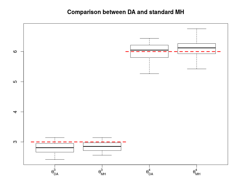
Figure 5 details the MCMC outcome in the first case. The box-plots represent approximations to the marginal posterior distributions of two coefficients in a logistic regression based on simulated data. Those box-plots are quite similar in terms of both mean values and variability when comparing the standard Metropolis–Hastings algorithm with the standard Metropolis–Hastings algorithm with delayed acceptance. Both approximations are concentrated around the true values of the parameters.
4.1.2 Higgs Boson Data
ATLAS (A Toroidal LHC Apparatus) is a particle detector experiment constructed at the Large Hadron Collider (LHC), at CERN, and designed to search for new particles based on collisions of protons of extraordinarily high energy. The ATLAS experiment has recently observed [1] evidence for the Higgs boson decaying into two tau particles, but the background noise is considerably high. The ATLAS team then launched a machine learning challenge through the Kaggle33 3 https://www.kaggle.com depository, providing public data in the form of simulations reproducing the behaviour of the ATLAS experiment. This training dataset is made of 25,0000 events with 30 feature columns and a binary label stating if the event is a real signal of decay or just background noise. Modelling this dataset through a logit model is thus adequate.
We compared the combined algorithm of delayed acceptance and prefetching from Section 4.1.1 with regular dynamic prefetching as in [25], both with iterations after burn-in iterations. The portion of the sample used in the first acceptance ratio (and used to approximate the remaining likelihood at the next step) is 5%, i.e. 12500 points. The proposal for the logit coefficients is again a normal distribution with covariance matrix the asymptotic covariance of the MLE estimator, obtained from a subset of the data, and adapted during the burn-in phase.
In this experiment, we used cores in parallel and obtained that the delayed acceptance algorithm runs almost 6 times faster than its classic counterpart, in line with the average number of draws per iteration obtained (159.22 for delayed acceptance versus just 29.03 for the standard version). The acceptance rate, although quite low for both the algorithms, remained constant through repetitions for both the methods, namely around 0.5%, and so was the relative ESS, around .
Once again, the approximations obtained with both algorithms are very close. In this case, a huge sample size leads to highly concentrated posterior distributions. We have chosen to represent only the posteriors of two parameters, for clarity’s sake, although all other parameters show a substantial similarity between both algorithms.

4.2 Mixture Model
Consider a standard mixture model [15] with a fixed number of components
| (6) |
This standard setting nonetheless offers a computational challenge in that the reference objective Bayesian approach based on the Fisher information and the associated Jeffreys prior [13, 20] is not readily available for computational reasons and has thus not being implemented so far. Proxys using the Jeffreys priors of the component of (6) have been proposed instead in the past, with the drawback that since they always lead to improper posteriors, ad hoc corrections had to implemented [6, 22, 24].
When relying instead on dependent improper priors, it is less clear that the improperness of the posterior distribution happens. For instance, we consider the genuine Jeffreys prior for the complete set of parameters in (6), derived from the Fisher information matrix for the whole model. While establishing the analytical properness of the associated posterior is beyond the goal of the current paper (work in progress), we handle large enough samples to posit that a sufficient number of observations is allocated to each component and hence the likelihood function dominates the prior distribution. (In the event the posterior remains improper, the associated MCMC algorithm should exhibit a transient behaviour.)
We therefore argue this is an appropriate and realistic example for implementing delayed acceptance since the computation of the prior density is clearly costly, relying on many integrals of the form:
| (7) |
Indeed, integrals of this form cannot be computed analytically and thus their derivation involve numerical or Monte Carlo integration. We are therefore in a setting where the prior ratio—as opposed to the more common case of the likelihood ratio—is the costly part of the target evaluated in the Metropolis-Hastings acceptance ratio. Moreover, since the Jeffreys prior involves a determinant, there is no easy way to split the computation further than ”prior times likelihood”. Indeed, the likelihood function is straightforward to compute. Hence, the delayed acceptance algorithm can be applied by simply splitting between the prior and the likelihood ratios, the later being computed first. Since in this setting the prior is (according to simulation studies) improper, picking the acceptance ratio at the second step solely on the prior distribution may create trapping states in practice, even though the method would remain valid. We therefore opt to the stabilising alternative to keep a small fraction (chosen to be 2% in our implementation) of the likelihood to regularise this second acceptance ratio by multiplication with the prior. This choice translates into Algorithm 4.
Set and
- 1.
Simulate ;
- 2.
Simulate and set ;
- 3.
if , repeat the current parameter value and return to 1;
else set ; - 4.
if accept ;
else repeat the current parameter value and return to 1.
An experiment comparing a standard Metropolis–Hastings implementation with a Metropolis–Hastings version relying on delayed acceptance (again, with and without prefetching) is summarised in Table 2 and in Figures 7–12. When implementing the prefetching option we have only resorted to a maximum of 8 processors (for availability reasons). Data was simulated from the following Gaussian mixture model:
| (8) |
The graphs in Figures 7–12 report on the resulting approximations to the marginal posterior distributions of the parameters of a three-component Gaussian mixture, obtained with a Metropolis-Hastings algorithm in the first instances and with the delayed acceptance algorithm in the second instance (in both cases, in conjunction with prefetching). Both raw MCMC sequences and histograms show a remarkable similarity in their approximation to the posterior distributions. In particular, the estimation of the parameters of the third component (which has the highest variance) shows the same highest variability in both the cases. As an aside we also notice that label switching does occur there [12].
| Algorithm | ESS (aver.) | ESS (var) | time (aver.) | time (var) | Acceptance rate |
|---|---|---|---|---|---|
| MH | 168.85 | 62.37 | 517.60 | 0.51 | 0.50 |
| MH + DA | 112.74 | 2155.89 | 322.38 | 28.69 | 0.43 |
| MH + pref. | 173.30 | 506.57 | 225.18 | 0.03 | 0.50 |
| MH + DA + pref. | 150.18 | 841.06 | 192.65 | 76.28 | 0.43 |


The delayed acceptance algorithm naturally exhibit a smaller acceptance rate (around when compared with a standard MCMC algorithm with no parallelisation (around ), but the difference is minor.
Furthermore, this lesser efficiency is to be balanced by the major improvement that the computational time is times less with MCMC with delayed acceptance with respect to a standard MCMC with to for simulations and a sample size , while the gain is even higher while using prefetching (the computational time is reduced two times). The average number of draws obtained when using delayed acceptance with prefetching is with respect to when using only prefetching, giving the same indication that the reduction in computing time.
Overall, the accepted values are highly correlated in all the cases; in particular, when using the delayed acceptance algorithm the effective sample size is around times less than when using a standard Metropolis–Hastings. The computational time of the delayed acceptance algorithm with prefetching is 3 times less than the standard MCMC, against a less strong reduction of the effective sample.
5 Conclusion
While the choice of splitting the target distribution into pieces ultimately depends on the respective costs of computing the said pieces and of reducing the overall acceptance rate, this generic alternative to the standard Metropolis–Hastings approach should be considered on a customary basis since it requires very little modification in programming and since it can be tested against the basic version.
The delayed acceptance algorithm presented in (2) could broadly decrease the computational time per se; a counterweight is the reduced acceptance rate, nevertheless the examples presented in Section 4 suggest that the gain in terms of computational time is not linear with respect to the reduction of the acceptance rate.
Furthermore, our delayed acceptance algorithm does naturally merge with the widening range of prefetching techniques, in order to make use of parallelisation and reduce the overall computational time even more significantly.
Most settings of interest are open to take advantage of the proposed method, if mostly when either the likelihood or the prior distribution are costly to evaluate. The setting when the likelihood function can be factorised in an useful way represents the best gain brought by our solution, in terms of computational time, as it mainly exploits the parallelisation.
Acknowledgments
Thanks to Christophe Andrieu for very helpful advice in validating the multi-step acceptance procedure. The massive help provided by Jean-Michel Marin and Pierre Pudlo towards an implementation on a large cluster has been fundamental in the completion of this work. Christian P. Robert research is partly financed by Agence Nationale de la Recherche (ANR, 212, rue de Bercy 75012 Paris) on the 2012–2015 ANR-11-BS01-0010 grant “Calibration” and by a 2010–2015 senior chair grant of Institut Universitaire de France.
References
- [1] The ATLAS collaboration (2013). Evidence for Higgs Boson Decays to the Final State with the ATLAS Detector. Tech. Rep. ATLAS-CONF-2013-108, CERN, Geneva.
- [2] Andrieu, C. and Roberts, G. (2009). The pseudo-marginal approach for efficient Monte Carlo computations. Ann. Statist., 37 697–725.
- [3] Angelino, E., Kohler, E., Waterland, A., Seltzer, M. and Adams, R. (2014). Accelerating MCMC via parallel predictive prefetching. arXiv preprint arXiv:1403.7265.
- [4] Brockwell, A. (2006). Parallel Markov chain Monte Carlo simulation by pre-fetching. J. Comput. Graphical Stat., 15 246–261.
- [5] Christen, J. and Fox, C. (2005). Markov chain Monte Carlo using an approximation. Journal of Computational and Graphical Statistics, 14 795–810.
- [6] Diebolt, J. and Robert, C. (1994). Estimation of finite mixture distributions by Bayesian sampling. J. Royal Statist. Society Series B, 56 363–375.
- [7] Doucet, A., Pitt, M., Deligiannidis, G. and Kohn, R. (2012). Efficient implementation of Markov chain Monte Carlo when using an unbiased likelihood estimator. ArXiv e-prints. 1210.1871.
- [8] Fox, C. and Nicholls, G. (1997). Sampling conductivity images via MCMC. The Art and Science of Bayesian Image Analysis 91–100.
- [9] Gelman, A., Gilks, W. and Roberts, G. (1996). Efficient Metropolis jumping rules. In Bayesian Statistics 5 (J. Berger, J. Bernardo, A. Dawid, D. Lindley and A. Smith, eds.). Oxford University Press, Oxford, 599–608.
- [10] Girolami, M. and Calderhead, B. (2011). Riemann manifold Langevin and Hamiltonian Monte Carlo methods. Journal of the Royal Statistical Society: Series B (Statistical Methodology), 73 123–214.
- [11] Jacob, P., Robert, C. and Smith, M. (2011). Using parallel computation to improve independent Metropolis–Hastings based estimation. J. Comput. Graph. Statist., 20 616–635.
- [12] Jasra, A., Holmes, C. and Stephens, D. (2005). Markov Chain Monte Carlo methods and the label switching problem in Bayesian mixture modeling. Statist. Sci., 20 50–67.
- [13] Jeffreys, H. (1939). Theory of Probability. 1st ed. The Clarendon Press, Oxford.
- [14] Korattikara, A., Chen, Y. and Welling, M. (2013). Austerity in MCMC land: Cutting the Metropolis-Hastings budget. arXiv preprint arXiv:1304.5299.
- [15] MacLachlan, G. and Peel, D. (2000). Finite Mixture Models. John Wiley, New York.
- [16] Neal, R. (1997). Markov chain Monte Carlo methods based on ‘slicing’ the density function. Tech. rep., University of Toronto.
- [17] Neal, R. (2012). MCMC using Hamiltonian dynamics. arXiv preprint arXiv:1206.1901.
- [18] Neiswanger, W., Wang, C. and Xing, E. (2013). Asymptotically exact, embarrassingly parallel MCMC. arXiv preprint arXiv:1311.4780.
- [19] Peskun, P. (1973). Optimum Monte Carlo sampling using Markov chains. Biometrika, 60 607–612.
- [20] Robert, C. (2001). The Bayesian Choice. 2nd ed. Springer-Verlag, New York.
- [21] Robert, C. and Casella, G. (2004). Monte Carlo Statistical Methods. 2nd ed. Springer-Verlag, New York.
- [22] Roeder, K. and Wasserman, L. (1997). Practical Bayesian density estimation using mixtures of normals. J. American Statist. Assoc., 92 894–902.
- [23] Scott, S., Blocker, A., Bonassi, F., Chipman, H., George, E. and McCulloch, R. (2013). Bayes and big data: The consensus Monte Carlo algorithm. EFaBBayes 250” conference, 16.
- [24] Stephens, M. (1997). Bayesian Methods for Mixtures of Normal Distributions. Ph.D. thesis, University of Oxford.
- [25] Strid, I. (2010). Efficient parallelisation of Metropolis–Hastings algorithms using a prefetching approach. Computational Statistics & Data Analysis, 54 2814––2835.
- [26] Tierney, L. (1994). Markov chains for exploring posterior distributions (with discussion). Ann. Statist., 22 1701–1786.
- [27] Tierney, L. and Mira, A. (1998). Some adaptive Monte Carlo methods for Bayesian inference. Statistics in Medicine, 18 2507–2515.
- [28] Wang, X. and Dunson, D. (2013). Parallel MCMC via Weierstrass sampler. arXiv preprint arXiv:1312.4605.