Maximum Likelihood-based Online Adaptation of Hyper-parameters in CMA-ES
Abstract
The Covariance Matrix Adaptation Evolution Strategy (CMA-ES) is widely accepted as a robust derivative-free continuous optimization algorithm for non-linear and non-convex optimization problems. CMA-ES is well known to be almost parameterless, meaning that only one hyper-parameter, the population size, is proposed to be tuned by the user. In this paper, we propose a principled approach called self-CMA-ES to achieve the online adaptation of CMA-ES hyper-parameters in order to improve its overall performance. Experimental results show that for larger-than-default population size, the default settings of hyper-parameters of CMA-ES are far from being optimal, and that self-CMA-ES allows for dynamically approaching optimal settings.
1 Introduction
The Covariance Matrix Adaptation Evolution Strategy (CMA-ES [5]) is a continuous optimizer which only exploits the ranking of estimated candidate solutions to approach the optimum of an objective function . CMA-ES is also invariant w.r.t. affine transformations of the decision space, explaining the known robustness of the algorithm. An important practical advantage of CMA-ES is that all hyper-parameters thereof are defined by default with respect to the problem dimension . Practically, only the population size is suggested to be tuned by the user, e.g. when a parallelization of the algorithm is considered or the problem at hand is known to be multi-modal and/or noisy [1, 8]. Other hyper-parameters have been provided robust default settings (depending on and ), in the sense that their offline tuning allegedly hardly improves the CMA-ES performance for unimodal functions. In the meanwhile, for multi-modal functions it is suggested that the overall performance can be significantly improved by offline tuning of and multiple stopping criteria [16, 11]. Additionally, it is shown that CMA-ES can be improved by a factor up to 5-10 by the use of surrogate models on unimodal ill-conditioned functions [14]. This suggests that the CMA-ES performance can be improved by better exploiting the information in the evaluated samples .
This paper focuses on the automatic online adjustment of the CMA-ES hyper-parameters. The proposed approach, called self-CMA-ES, relies on a second CMA-ES instance operating on the hyper-parameter space of the first CMA-ES, and aimed at increasing the likelihood of generating the most successful samples x in the current generation. The paper is organized as follows. Section 2 describes the original -CMA-ES. self-CMA-ES is described in Section 3 and its experimental validation is discussed in Section 4 comparatively to related work. Section 5 concludes the paper.
2 Covariance Matrix Adaptation Evolution Strategy
The Covariance Matrix Adaptation Evolution Strategy [6, 7, 5] is acknowledgedly the most popular and the most efficient Evolution Strategy algorithm.
The original ()-CMA-ES (Algorithm 1) proceeds as follows. At the -th iteration, a Gaussian distribution is used to generate candidate solution , for (line 5):
| (1) |
where the mean of the distribution can be interpreted as the current estimate of the optimum of function , is a (positive definite) covariance matrix and is a mutation step-size. These solutions are evaluated according to (line 6). The new mean of the distribution is computed as a weighted sum of the best individuals out of the ones (line 7). Weights are used to control the impact of selected individuals, with usually higher weights for top ranked individuals (line 1).
The adaptation of the step-size , inherited from the Cumulative Step-Size Adaptation Evolution Strategy (CSA-ES [6]), is controlled by the evolution path . Successful mutation steps (line 8) are tracked in the sampling space, i.e., in the isotropic coordinate system defined by the eigenvectors of the covariance matrix . To update the evolution path , i) a decay/relaxation factor is used to decrease the importance of previous steps; ii) the step-size is increased if the length of the evolution path is longer than the expected length of the evolution path under random selection ; iii) otherwise it is decreased (line 13). Expectation of is approximated by . A damping parameter controls the change of the step-size.
The covariance matrix update consists of two parts (line 12): a rank-one update [7] and a rank- update [5]. The rank-one update computes the evolution path of successful moves of the mean of the mutation distribution in the given coordinate system (line 10), along the same lines as the evolution path of the step-size. To stall the update of when increases rapidly, a trigger is used (line 9).
The rank- update computes a covariance matrix as a weighted sum of the covariances of successful steps of the best individuals (line 11). Covariance matrix C itself is replaced by a weighted sum of the rank-one (weight [7]) and rank- (weight [5]) updates, with and positive and .
While the optimal parameterization of CMA-ES remains an open problem, the default parameterization is found quite robust on noiseless unimodal functions [5], which explains the popularity of CMA-ES.
3 The self-CMA-ES
The proposed self-CMA-ES approach is based on the intuition that the optimal hyper-parameters of CMA-ES at time should favor the generation of the best individuals at time , under the (strong) assumption that an optimal parameterization and performance of CMA-ES in each time will lead to the overall optimal performance.
Formally, this intuition leads to the following procedure. Let denote the hyper-parameter vector used for the optimization of objective at time (CMA-ES stores its state variables and internal parameters of iteration in and the ’.’-notation is used to access them). At time , the best individuals generated according to are known to be the top-ranked individuals , where stands for the -th best individual w.r.t. . Hyper-parameter vector would thus have been all the better, if it had maximized the probability of generating these top individuals.
Along this line, the optimization of is conducted using a second CMA-ES algorithm, referred to as auxiliary CMA-ES as opposed to the one concerned with the optimization of , referred to as primary CMA-ES. The objective of the auxiliary CMA-ES is specified as follows:
Given: hyper-parameter vector and points evaluated by primary CMA-ES at steps (noted as in Algorithm 2),
Find: such that i) backtracking the primary CMA-ES to its state at time ; ii) replacing by , would maximize the likelihood of for .
The auxiliary CMA-ES might thus tackle the maximization of computed as the weighed log-likelihood of the top-ranked individuals at time :
| (2) |
where and by construction
| (3) |
where is the covariance matrix multiplied by and is its determinant.
While the objective function for the auxiliary CMA-ES defined by Eq. (2) is mathematically sound, it yields a difficult optimization problem; firstly the probabilities are scale-sensitive; secondly and overall, in a worst case scenario, a single good but unlikely solution may lead the optimization of astray.
Therefore, another optimization objective is defined for the auxiliary CMA-ES, where measures the agreement on for between i) the order defined from ; ii) the order defined from their likelihood conditioned by (Algorithm 3). Procedure ReproduceGenerationCMA in Algorithm 3 updates the strategy parameters described from line 7 to line 14 in Algorithm 1 using already evaluated solutions stored in . Line 4 computes the Mahalanobis distance, division by step-size is not needed since only ranking will be considered in line 5 (decreasing order of Mahalanobis distances corresponds to increasing order of log-likelihoods). Line 6 computes a weighted sum of ranks of likelihoods of best individuals.
Finally, the overall scheme of self-CMA-ES (Algorithm 2) involves two interdependent CMA-ES optimization algorithms, where the primary CMA-ES is concerned with optimizing objective , and the auxiliary CMA-ES is concerned with optimizing objective , that is, optimizing the hyper-parameters of the primary CMA-ES11 1 This scheme is actually inspired from the one proposed for surrogate-assisted optimization [13], where the auxiliary CMA-ES was in charge of optimizing the surrogate learning hyper-parameters.. Note that self-CMA-ES is not per se a “more parameterless“ algorithm than CMA-ES, in the sense that the user is still invited to modify the population size . The main purpose of self-CMA-ES is to achieve the online adaptation of the other CMA-ES hyper-parameters.
Specifically, while the primary CMA-ES optimizes (line 8), the auxiliary CMA-ES maximizes (line 9) by sampling and evaluating variants of . The updated mean of the auxiliary CMA-ES in the hyper-parameter space is used as a local estimate of the optimal hyper-parameter vector for the primary CMA-ES. Note that the auxiliary CMA-ES achieves a single iteration in the hyper-parameter space of the primary CMA-ES, with two motivations: limiting the computational cost of self-CMA-ES (which scales as times the time complexity of the CMA-ES), and preventing from overfitting the current sample .


4 Experimental Validation
The experimental validation of self-CMA-ES investigates the performance of the
algorithm comparatively to CMA-ES on the BBOB noiseless problems [4].
Both algorithms are launched in IPOP scenario of restarts when the CMA-ES is restarted
with doubled population size once stopping criteria [3] are met22
2
For the sake of reproducibility, the source code is available at
https://sites.google.com/site/selfcmappsn/.
The population size is chosen to be 100 for both CMA-ES and self-CMA-ES.
We choose this value (about 10 times larger than the default one, see the default parameters of CMA-ES in Algorithm 1) to investigate how sub-optimal the other CMA-ES hyper-parameters, derived from , are in such a case, and whether self-CMA-ES can
recover from this sub-optimality.
The auxiliary CMA-ES is concerned with optimizing hyper-parameters , and (Algorithm 1), responsible for the adaptation of the covariance matrix of the primary CMA-ES. These parameters range in subject to ; the constraint is meant to enforce a feasible C update for the primary CMA-ES (the decay factor of C should be in ). Infeasible hyper-parameter solutions get a very large penalty, multiplied by the sum of distances of infeasible hyper-parameters to the range of feasibility.
We set for and to 50. The internal computational complexity of self-CMA-ES thus is times larger than the one of CMA-ES without lazy update (being reminded that the internal time complexity is usually negligible compared to the cost per objective function evaluation).
4.1 Results
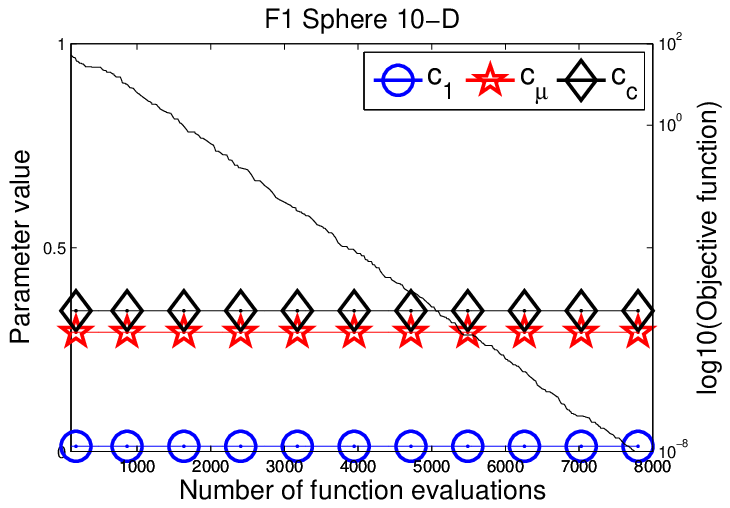
Figures 1 and 2 display the comparative performances of CMA-ES (left) and self-CMA-ES (right) on 10 and 20-dimensional Sphere, Rosenbrock, Rotated Ellipsoid and Sharp ridge functions from the noiseless BBOB testbed [4] (medians out of 15 runs). Each plot shows the value of the hyper-parameters (left y-axis) together with the objective function (in logarithmic scale, right y-axis). Hyper-parameters , and are constant and set to their default values for CMA-ES while they are adapted along evolution for self-CMA-ES.
In self-CMA-ES, the hyper-parameters are uniformly initialized in (therefore the medians are close to 0.45) and they gradually converge to values which are estimated to provide the best update of the covariance matrix w.r.t. the ability to generate the current best individuals. It is seen that these values are problem and dimension-dependent. The values of are always much smaller than but are comparable to the default . The values of and and are almost always larger than the default ones; this is not a surprise for and , as their original default values are chosen in a rather conservative way to prevent degeneration of the covariance matrix.
Several interesting observations can be made about the dynamics of the parameter values. The value of is high most of the times on the Rosenbrock functions, but it decreases toward values similar to those of the Sphere functions, when close to the optimum. This effect is observed on most problems; indeed, on most problems fast adaptation of the covariance matrix will improve the performance in the beginning, while the distribution shape should remain stable when the covariance matrix is learned close to the optimum.
The overall performance of self-CMA-ES on the considered problems is comparable to that of CMA-ES, with a speed-up of a factor up to 1.5 on Sharp Ridge functions. The main result is the ability of self-CMA-ES to achieve the online adaptation of the hyper-parameters depending on the problem at hand, side-stepping the use of long calibrated default settings33 3 , , ..
4.2 Discussion
self-CMA-ES offers a proof of concept for the online adaptation of three CMA-ES hyper-parameters in terms of feasibility and usefulness. Previous studies on parameter settings for CMA-ES mostly considered offline tuning (see, e.g., [16, 11]) and theoretical analysis dated back to the first papers on Evolution Strategies. The main limitation of these studies is that the suggested hyper-parameter values are usually specific to the (class of) analyzed problems. Furthermore, the suggested values are fixed, assuming that optimal parameter values remain constant along evolution. However, when optimizing a function whose landscape gradually changes when approaching the optimum, one may expect optimal hyper-parameter values to reflect this change as well.
Studies on the online adaptation of hyper-parameters (apart from , m and C) usually consider population size in noisy [2], multi-modal [1, 12] or expensive [9] optimization. A more closely related approach was proposed in [15] where the learning rate for step-size adaptation is adapted in a stochastic way similarly to Rprop-updates [10].
5 Conclusion and Perspectives
This paper proposes a principled approach for the self-adaptation of CMA-ES hyper-parameters, tackled as an auxiliary optimization problem: maximizing the likelihood of generating the best sampled solutions. The experimental validation of self-CMA-ES shows that the learning rates involved in the covariance matrix adaptation can be efficiently adapted on-line, with comparable or better results than CMA-ES. It is worth emphasizing that matching the performance of CMA-ES, the default setting of which represent a historical consensus between theoretical analysis and offline tuning, is nothing easy.
The main novelty of the paper is to offer an intrinsic assessment of the algorithm internal state, based on retrospective reasoning (given the best current solutions, how could the generation of these solutions have been made easier) and on one assumption (the optimal hyper-parameter values at time are ”sufficiently good“ at time ). Further work will investigate how this intrinsic assessment can support the self-adaptation of other continuous and discrete hyper-parameters used to deal with noisy, multi-modal and constrained optimization problems.
Acknowledgments
We acknowledge anonymous reviewers for their constructive comments. This work was supported by the grant ANR-2010-COSI-002 (SIMINOLE) of the French National Research Agency.
References
- [1] A. Auger and N. Hansen. A Restart CMA Evolution Strategy With Increasing Population Size. In IEEE Congress on Evolutionary Computation, pages 1769–1776. IEEE Press, 2005.
- [2] H.-G. Beyer and M. Hellwig. Controlling population size and mutation strength by meta-es under fitness noise. In Proceedings of the Twelfth Workshop on Foundations of Genetic Algorithms XII, FOGA XII ’13, pages 11–24. ACM, 2013.
- [3] N. Hansen. Benchmarking a BI-population CMA-ES on the BBOB-2009 function testbed. In GECCO Companion, pages 2389–2396, 2009.
- [4] N. Hansen, A. Auger, S. Finck, and R. Ros. Real-Parameter Black-Box Optimization Benchmarking 2010: Experimental Setup. Technical report, INRIA, 2010.
- [5] N. Hansen, S. Müller, and P. Koumoutsakos. Reducing the time complexity of the derandomized evolution strategy with covariance matrix adaptation (CMA-ES). Evolutionary Computation, 11(1):1–18, 2003.
- [6] N. Hansen and A. Ostermeier. Adapting Arbitrary Normal Mutation Distributions in Evolution Strategies: The Covariance Matrix Adaptation. In International Conference on Evolutionary Computation, pages 312–317, 1996.
- [7] N. Hansen and A. Ostermeier. Completely Derandomized Self-Adaptation in Evolution Strategies. Evolutionary Computation, 9(2):159–195, June 2001.
- [8] N. Hansen and R. Ros. Benchmarking a weighted negative covariance matrix update on the BBOB-2010 noisy testbed. In GECCO ’10: Proceedings of the 12th annual conference comp on Genetic and evolutionary computation, pages 1681–1688, New York, NY, USA, 2010. ACM.
- [9] F. Hoffmann and S. Holemann. Controlled Model Assisted Evolution Strategy with Adaptive Preselection. In International Symposium on Evolving Fuzzy Systems, pages 182–187. IEEE, 2006.
- [10] C. Igel and M. Hüsken. Empirical evaluation of the improved rprop learning algorithms. Neurocomputing, 50:105–123, 2003.
- [11] T. Liao and T. Stützle. Benchmark results for a simple hybrid algorithm on the CEC 2013 benchmark set for real-parameter optimization. In IEEE Congress on Evolutionary Computation (CEC), pages 1938–1944. IEEE press, 2013.
- [12] I. Loshchilov, M. Schoenauer, and M. Sebag. Alternative Restart Strategies for CMA-ES. In V. C. et al., editor, Parallel Problem Solving from Nature (PPSN XII), LNCS, pages 296–305. Springer, September 2012.
- [13] I. Loshchilov, M. Schoenauer, and M. Sebag. Self-Adaptive Surrogate-Assisted Covariance Matrix Adaptation Evolution Strategy. In Genetic and Evolutionary Computation Conference (GECCO), pages 321–328. ACM Press, July 2012.
- [14] I. Loshchilov, M. Schoenauer, and M. Sebag. Intensive Surrogate Model Exploitation in Self-adaptive Surrogate-assisted CMA-ES (saACM-ES). In Genetic and evolutionary computation conference, pages 439–446. ACM, 2013.
- [15] T. Schaul. Comparing natural evolution strategies to bipop-cma-es on noiseless and noisy black-box optimization testbeds. In Genetic and evolutionary computation conference companion, pages 237–244. ACM, 2012.
- [16] S. Smit and A. Eiben. Beating the ‘world champion’ Evolutionary Algorithm via REVAC Tuning. In IEEE Congress on Evolutionary Computation, pages 1–8, 2010.