跳到论文正文
W Papers独立论文阅读器 arXiv:1406.2591 论文正文 计算阅读时间 · 0%
引用这篇论文根据当前论文元数据生成,正式投稿前建议核对。


License: arXiv.org perpetual non-exclusive license
arXiv:1406.2591v3 [hep-ph] 18 Nov 2014

Renormalization-group improved predictions for Higgs boson production at large pTp_{T}

Fa Peng Huang Affiliation: School of Physics and State Key Laboratory of Nuclear Physics and Technology, Peking University, Beijing, 100871, China    Chong Sheng Li Note: Electronic address: csli@pku.edu.cn Affiliation: School of Physics and State Key Laboratory of Nuclear Physics and Technology, Peking University, Beijing, 100871, China Affiliation: Center for High Energy Physics, Peking University, Beijing, 100871, China    Hai Tao Li Affiliation: School of Physics and State Key Laboratory of Nuclear Physics and Technology, Peking University, Beijing, 100871, China    Jian Wang Affiliation: PRISMA Cluster of Excellence &\& Mainz Institut for Theoretical Physics, Johannes Gutenberg University, D-55099 Mainz, Germany
Abstract

We study the next-to-next-to-leading logarithmic order resummation for the large pTp_{T} Higgs boson production at the LHC in the framework of soft-collinear effective theory. We find that the resummation effects reduce the scale uncertainty significantly and decrease the QCD NLO results by about 11%11\% in the large pTp_{T} region. The finite top quark mass effects and the effects of the NNLO singular terms are also discussed.

pacs
12.38.Cy,14.80.Bn

I Introduction

In the standard model (SM), the Higgs boson is predicted by the Higgs mechanism in which the would-be Goldstones become the longitudinal components of the W and Z bosons. Although the existence of Higgs boson has been proposed for a long time, searching for this particle in the experiments has failed until the recent discovery at the LHC [1, 2]. In general, the Higgs boson may not be responsible for the mass origin of the fermions, and the current experimental data still allow the couplings of the Higgs boson with the fermions to deviate from the SM ones, especially, the coupling of the Higgs boson to the top quark [3]. Therefore, precise measurements of the couplings of the Higgs boson with other SM particles will test the Higgs mechanism in the SM [4, 5, 6, 7].

The global fit method with current experiment data about the Higgs boson production and decay in various channels only provides indirect information on the top quark Yukawa coupling, which suffers from ambiguities from unknown new particles propagating in the loops. The most direct process to determine the coupling of the Higgs boson to the top quark is the t​t¯t\bar{t} associated production p​p→t​t¯​Hpp\to t\bar{t}H and single top associated production p​p→t​j​Hpp\to tjH. However, the current abilities to measure the coupling of Higgs boson to the top quark through t​t¯t\bar{t} associated production are still weak [3, 8] because of its small production cross section and complicated final states with copious decay products. The single top associated production has even smaller cross section because of the electro-weak interactions there, and is very challenging to measure.

Recently, a complementary method to determine the coupling of the Higgs boson to the top quark has been proposed in Refs. [5, 6, 7] by investigating the large pTp_{T} behavior of the Higgs boson in the process p​p→H+Xpp\to H+X with H→Z​Z∗→l+​l−​l+​l−H\to ZZ^{*}\to l^{+}l^{-}l^{+}l^{-}. This method is feasible because the top quark mass can not be taken to be infinity when the Higgs boson has a large pTp_{T}. The top quark Yukawa coupling can be detected from the measurement of the variable [5]

r±=N+/N−σSM+/σSM−,r_{\pm}=\frac{N^{+}/N^{-}}{\sigma_{\rm SM}^{+}/\sigma_{\rm SM}^{-}}, (1)

where N±N^{\pm} is the number of events in which the Higgs boson pTp_{T} is larger or smaller than a critical value PTP_{T}, for example, PT=P_{T}=300 GeV. σSM±\sigma_{\rm SM}^{\pm} is the corresponding theoretical predictions in the SM. It is pointed out that [5] the KK factor, defined as the ratio of higher order results to the LO ones, for the Higgs boson pTp_{T} distribution is roughly pTp_{T} independent and very large, about 2, and that the resummation effects are negligible in the pTp_{T} range they considered. All these arguments are based on the calculation by the HqT program [9]. However, the resummation scheme used in the HqT program is only valid in the small pTp_{T} region, which is much less than 100 GeV. The resummation prediction on the Higgs boson pTp_{T} distribution in the large pTp_{T} region, larger than 100 GeV, is investigated using the traditional method at next-to-leading-logarithm (NLL) [10]. The resumed logarithms are different in the small and large pTp_{T} regions. When the Higgs boson pTp_{T} is small, the threshold region is defined as z=MH2/s→1z=M_{H}^{2}/s\to 1, where s\sqrt{s} is the center-of-mass energy of the colliding partons. In the threshold region, only the soft gluon radiation is allowed, which leads to large logarithms αsn​ln2​n−m⁡(1−z)\alpha_{s}^{n}\ln^{2n-m}(1-z). In contrast, in the large pTp_{T} regions, the large logarithms are αsn​ln2​n−m⁡(1−y)\alpha_{s}^{n}\ln^{2n-m}(1-y) with y=(pT+mT)2/sy=(p_{T}+m_{T})^{2}/s, where mT=pT2+MH2m_{T}=\sqrt{p_{T}^{2}+M_{H}^{2}} [10]. It is easy to observe that y→1y\to 1 does not necessarily lead to z→1z\to 1, which means that the HqT program can not resum the large logarithms in the large pTp_{T} regions.

Notice that when the recoiling hardest jet against the Higgs boson is observed and additional jets are vetoed, there is a new kind of large Sudakov logarithms αsn​ln2​n−m​pT/pTveto\alpha_{s}^{n}\ln^{2n-m}p_{T}/p_{T}^{\rm veto}, which can be resummed [11, 12, 13]. If the mass of the jet is also measured, denoted as mJm_{J}, additional logarithms lnn⁡mJ2/pJ2\ln^{n}m_{J}^{2}/p_{J}^{2} have been resummed up to next-to-next-to-leading-logarithm (NNLL) [14].

In this paper, we provide the resummed prediction for p​p→H+Xpp\to H+X at large pTp_{T} regions up to NNLL, without explicit observation of a jet, in contract with the case in [14]. We will work in the soft-collinear effective theory (SCET) [15, 16, 17, 18, 19]. In the threshold limits of large pTp_{T} Higgs boson production, the final state radiations and beam remnants are highly suppressed which leads to final states consisting of a Higgs boson and an inclusive jet, as well as the remaining soft radiations, and therefore to the appearance of the large logarithms in the cross section. Then the resummation effects should be taken into account to obtain more precise predictions. The preliminarily theoretical NNLO analyses have been perfromed in Ref. [20]. The resummation formalism in SCET is different from that used in Ref. [10]. In the threshold region, the partonic cross section can be factorized to a hard function times a convolution between jet and soft functions. Each part has a explicit theoretical field definition which can be calculated perturbatively. In particular, each function contains only a single energy scale so that there is no potential large logarithms in each of them. The relative scale hierarchy between different functions is alleviated by running from one to the other via renormalization group equations. As a consequence, the large logarithms of the ratio of the different scales can be resummed to all orders.

In principle, the top quark mass should be kept to be finite in all the theoretical predictions in the large pTp_{T} regions [21, 22, 5, 7]. But because of the difficulty in calculating massive loops, this is achieved only for the LO result [23, 24] and the NLO total cross section expanded in MH/mtM_{H}/m_{t}[25]. The differential cross section is calculated only in the large top quark limit up to NLO [26, 21, 27, 28, 21]. More recently, a big progress is made by computing the NNLO total cross section of the sub-process g​g→H+jgg\to H+j [29]. Therefore, an approximated differential cross section with finite top quark mass beyond the LO is usually used, which is obtained by multiplying the LO differential cross section with finite top quark mass with a differential KK factor, as done in Ref. [30]. We will take into account the finite top quark mass effects in the resummation predictions following this method.

The precision prediction on Higgs boson production at large pTp_{T} regions can not only test the top quark Yukawa coupling discussed above, but also be a probe of the new physics. For example, in the SM the large transverse momentum spectrum of the Higgs boson produced in gluon fusion can be quite different from one of the minimal supersymmetric standard model [31, 32]. Light particles beyond the SM can be probed via the ratio of the partially integrated Higgs transverse momentum distribution to the inclusive rate [33].

This paper is organized as follows. In Sec. II, we analyze the kinematics of the Higgs boson and one jet associated production and give the definition of the threshold region. In Sec. III, we present the factorization and resummation formalism in momentum space using SCET. In Sec. IV, we present the hard function, jet function and soft functions at NLO. Then, we study the scale independence of the final result analytically. In Sec. V, we discuss the numerical results for this process at the LHC. We conclude in Sec. VI.

II Analysis of kinematics

First of all, we introduce the relevant kinematical variables needed in our analysis. The dominant partonic processes for the Higgs boson and one jet production are g​g→g​Hgg\rightarrow gH, g​q→g​Hgq\rightarrow gH and g​q¯→q¯​Hg\bar{q}\rightarrow\bar{q}H. The LO Feynman diagrams for the g​g→g​Hgg\rightarrow gH process are shown in Fig. 1.

Refer to caption
Figure 1: LO Feynman diagrams for the gg channel.

It is convenient to define two lightlike vectors along the beam directions, nan_{a} and nbn_{b}, which are related by na=n¯bn_{a}=\bar{n}_{b}. Then, we introduce initial collinear fields along nan_{a} and nbn_{b} to describe the collinear particles in the beam directions. In the center-of-mass (c.m.) frame of the hadronic collision, the momenta of the incoming hadrons are given by

Paμ=Ec.m.​naμ2,Pbμ=Ec.m.​nbμ2.P^{\mu}_{a}=E_{\rm c.m.}\frac{n^{\mu}_{a}}{2},\qquad P^{\mu}_{b}=E_{\rm c.m.}\frac{n^{\mu}_{b}}{2}. (2)

Here Ec.m.E_{\rm c.m.} is the c.m. energy of the collider and we have neglected the masses of the hadrons. The momenta of the incoming partons, with a light-cone momentum fraction of the hadronic momentum, are

p~a=xa​Ec.m.​naμ2,p~b=xb​Ec.m.​nbμ2.\tilde{p}_{a}=x_{a}E_{\rm c.m.}\frac{n^{\mu}_{a}}{2},\qquad\tilde{p}_{b}=x_{b}E_{\rm c.m.}\frac{n^{\mu}_{b}}{2}. (3)

At the hadronic and partonic level, the momentum conservation gives

Pa+Pb=q+PX,P_{a}+P_{b}=q+P_{X}, (4)

and

p~a+p~b=q+pX,\tilde{p}_{a}+\tilde{p}_{b}=q+p_{X}, (5)

respectively, where qq is the momentum of the Higgs boson. We define the partonic jet with jet momentum pXp_{X} to be the set of all final state partons except the Higgs boson in the partonic processes, while the hadronic jet with jet momentum PXP_{X} contains all the hadrons as well as the beam remnants in the final state except the Higgs boson.

We also define the Mandelstam variables as

s=(Pa+Pb)2,u=(Pa−q)2,t=(Pb−q)2s=(P_{a}+P_{b})^{2},\quad u=(P_{a}-q)^{2},\quad t=(P_{b}-q)^{2} (6)

for hadrons, and

s^=(p~a+p~b)2,u^=(p~a−q)2,t^=(p~b−q)2\hat{s}=(\tilde{p}_{a}+\tilde{p}_{b})^{2},\quad\hat{u}=(\tilde{p}_{a}-q)^{2},\quad\hat{t}=(\tilde{p}_{b}-q)^{2} (7)

for partons, respectively. In terms of the Mandelstam variables, the hadronic and partonic threshold variables are defined as

S4\displaystyle S_{4} ≡\displaystyle\equiv PX2=s+t+u−MH2,\displaystyle P^{2}_{X}=s+t+u-M^{2}_{H}, (8)
s4\displaystyle s_{4} ≡\displaystyle\equiv pX2=s^+t^+u^−MH2,\displaystyle p^{2}_{X}=\hat{s}+\hat{t}+\hat{u}-M^{2}_{H}, (9)

where MHM_{H} is the mass of the Higgs boson. The hadronic threshold limit is defined as S4→0S_{4}\to 0 [34]. In this limit, the final state radiations and beam remnants are highly suppressed, which leads to final states consisting of a Higgs boson and an energetic jet, as well as the remaining soft radiations. Taking this limit requires xa→1,xb→1,s4→0x_{a}\to 1,\;x_{b}\to 1,\;s_{4}\to 0 simultaneously, and we get

S4\displaystyle S_{4} =\displaystyle= s4+s^​(1xa​xb−1)+(t^−MH2)​(1xb−1)+(u^−MH2)​(1xa−1)\displaystyle s_{4}+\hat{s}(\frac{1}{x_{a}x_{b}}-1)+(\hat{t}-M^{2}_{H})(\frac{1}{x_{b}}-1)+(\hat{u}-M^{2}_{H})(\frac{1}{x_{a}}-1) (10)
≈\displaystyle\approx s4+s^​(x¯a+x¯b)+(t^−MH2)​x¯b+(u^−MH2)​x¯a\displaystyle s_{4}+\hat{s}(\bar{x}_{a}+\bar{x}_{b})+(\hat{t}-M^{2}_{H})\bar{x}_{b}+(\hat{u}-M^{2}_{H})\bar{x}_{a}
≈\displaystyle\approx s4+(−t^)​x¯a+(−u^)​x¯b,\displaystyle s_{4}+(-\hat{t})\bar{x}_{a}+(-\hat{u})\bar{x}_{b},

where x¯a,b=1−xa,b\bar{x}_{a,b}=1-x_{a,b}. This expression can help to check the factorization scale invariance, which is shown in detail below. Near the partonic threshold, the boson must be recoiling against a jet and there is only phase space for the jet to be nearly massless. In this case, pX=p1+kp_{X}=p_{1}+k, where p1p_{1} is the momentum of the final state collinear partons forming the jet and kk is the momentum of the soft radiations.

We note that in both hadronic and partonic threshold limit, the Higgs boson is not forced to be produced at rest, i.e.i.e. it can have a large momentum. Actually, as the momentum of the Higgs boson becomes larger and larger, the final-state phase space lies more close to the threshold limit. We point that the definition of the partonic threshold limit s4/s^→0s_{4}/\hat{s}\to 0 is different from the case of y→1y\to 1 [10], as discussed in the introduction. They are equivalent to each other only if the momentum component pzp_{z} of the Higgs boson in the partonic c.m. frame vanishes.

For convenience, we can also write the threshold variable as

s4=pX2=(p~a+p~b−q)2=p12+2​k+​E1+𝒪⁡(k2),s_{4}=p^{2}_{X}=(\tilde{p}_{a}+\tilde{p}_{b}-q)^{2}=p^{2}_{1}+2k^{+}E_{1}+{\cal O}(k^{2}), (11)

where k+=n1⋅kk^{+}=n_{1}\!\cdot\!k, kk is the momentum of soft radiations, E1E_{1} is the energy of the jet and n1n_{1} is the lightlike vector associated with the jet direction. In the threshold limit (s4→0s_{4}\to 0), incomplete cancelation of the divergences between real and virtual corrections leads to singular distributions αsn​[lnm⁡(s4/MH2)/s4]+\alpha^{n}_{s}[\ln^{m}(s_{4}/M^{2}_{H})/s_{4}]_{+}, with m≤2​n−1m\leq 2n-1. It is the purpose of threshold resummation to sum up these contributions to all orders in αs\alpha_{s}.

The total cross section is given by

σ\displaystyle\sigma =\displaystyle= ∫d​xa​∫d​xb​∫d​t^​∫d​u^​fi/Pa​(μF,xa)​fj/Pb​(μF,xb)​12​s^​d​σ^i​jd​t^​d​u^\displaystyle\int dx_{a}\int dx_{b}\int d\hat{t}\int d\hat{u}f_{i/P_{a}}(\mu_{F},x_{a})f_{j/P_{b}}(\mu_{F},x_{b})\frac{1}{2\hat{s}}\frac{d\hat{\sigma}_{ij}}{d\hat{t}d\hat{u}}
=\displaystyle= ∫0pT,m​a​x2d​pT2​∫−ym​a​xym​a​xd​y​∫xb,m​i​n1d​xb​∫0s4m​a​xd​s4​12​(xb​s+u−MH2)​fi/Pa​(μF,xa)​fj/Pb​(μF,xb)​d​σ^i​jd​t^​d​u^,\displaystyle\int_{0}^{p^{2}_{T,max}}dp_{T}^{2}\int_{-y_{max}}^{y_{max}}dy\int_{x_{b,min}}^{1}dx_{b}\int_{0}^{s_{4}^{max}}ds_{4}\frac{1}{2(x_{b}s+u-M_{H}^{2})}f_{i/P_{a}}(\mu_{F},x_{a})f_{j/P_{b}}(\mu_{F},x_{b})\frac{d\hat{\sigma}_{ij}}{d\hat{t}d\hat{u}},

where we have changed the integration variables into the Higgs boson transverse momentum squared pT2p^{2}_{T}, rapidity yy, xbx_{b} and s4s_{4}. The regions of the integration variables are given by

pT,max2\displaystyle p^{2}_{T,{\rm max}} =\displaystyle= (s−MH2)24​s,\displaystyle\frac{(s-M_{H}^{2})^{2}}{4s},
ymax\displaystyle y_{\rm max} =\displaystyle= 12​ln​1+1−ξ1−1−ξ,\displaystyle\frac{1}{2}{\rm ln}\frac{1+\sqrt{1-\xi}}{1-\sqrt{1-\xi}},
xb,min\displaystyle x_{b,{\rm min}} =\displaystyle= −us+t−MH2,\displaystyle\frac{-u}{s+t-M_{H}^{2}},
s4max\displaystyle s_{4}^{\rm max} =\displaystyle= xb​(s+t−MH2)+u,\displaystyle x_{b}(s+t-M_{H}^{2})+u, (13)

with

ξ\displaystyle\xi =\displaystyle= 4​s​(pT2+MH2)(s+MH2)2,\displaystyle\frac{4s(p_{T}^{2}+M_{H}^{2})}{(s+M_{H}^{2})^{2}},
t\displaystyle t =\displaystyle= MH2−s​pT2+MH2​ey,\displaystyle M_{H}^{2}-\sqrt{s}\sqrt{p_{T}^{2}+M_{H}^{2}}e^{y},
u\displaystyle u =\displaystyle= MH2−s​pT2+MH2​e−y.\displaystyle M_{H}^{2}-\sqrt{s}\sqrt{p_{T}^{2}+M_{H}^{2}}e^{-y}. (14)

The other kinematical variables can be expressed in terms of these four integration variables.

III Factorization and Resummation Formalism in SCET

In the frame of SCET, we define a small expanded parameter λ=s4/Q\lambda=\sqrt{s_{4}}/Q (λ<<1\lambda<<1) in the threshold limit s4→0s_{4}\to 0. Here, Q is the characteristic energy of the hard scattering process. The momentum of a collinear particle scales as

collinear:pcμ∼Q⁡(1,λ2,λ),\mbox{collinear}:\quad p_{\mathrm{c}}^{\mu}\sim Q(1,\lambda^{2},\lambda), (15)

and the momentum of a soft particle scales as

soft:psμ∼Q⁡(λ2,λ2,λ2).\mbox{soft}:\quad p_{\mathrm{s}}^{\mu}\sim Q(\lambda^{2},\lambda^{2},\lambda^{2}). (16)

The soft fields scale as ψs∼λ3\psi_{\mathrm{s}}\sim\lambda^{3}, As∼λ2A_{\mathrm{s}}\sim\lambda^{2}, and the collinear fermion field ψc\psi_{\mathrm{c}} scales as λ\lambda. The light-cone components of the collinear gluon field AcμA_{\mathrm{c}}^{\mu} scale the same way as its momentum pcμp_{\mathrm{c}}^{\mu} in covariant gauge.

The soft gluon field are multipole expanded around x−x_{-} to maintain a consistent power counting in λ\lambda. Thus, the soft gluon operator depends only on x−μ=(n¯J⋅x)​nJμ2x_{-}^{\mu}=({\bar{n}_{J}}\cdot x)\frac{{n_{J}^{\mu}}}{2} at leading power, and its Fourier transform only depends on k+=nJ⋅kk_{+}={n_{J}}\cdot k. It is needed to mention that ps2∼Q2​λ2p_{s}^{2}\sim Q^{2}\lambda^{2} is of order of the jet mass and is assumed to be in the perturbative region.

In the limit of the infinite top quark mass, the effective Lagrangian of Higgs boson production via gluon fusion can be written as [26]

L=Ct​(mt,μ)​αs​(μ)12​π​Hv​T​r​(Gμ​ν​Gμ​ν),\textit{L}=C_{t}(m_{t},\mu)\frac{\alpha_{s}(\mu)}{12\pi}\frac{H}{\textit{v}}Tr(G_{\mu\nu}G^{\mu\nu}), (17)

with

Ct=1+11​αs​(μ)4​π,C_{t}=1+\frac{11\alpha_{s}(\mu)}{4\pi}, (18)

where CtC_{t} is the Wilson coefficient at αs\alpha_{s} order. The leading power effective operator of g​g→g​Hgg\rightarrow gH in SCET is as follows,

𝒪a​b​cα​β​γ​(x,t1,t2,tJ)\displaystyle\mathcal{O}_{abc}^{\alpha\beta\gamma}(x;t_{1},t_{2},t_{J}) =𝒜a⟂α​1​(x+t1​n¯1)​𝒜b⟂β​2​(x+t2​n¯2)​𝒜c⟂γ​J​(x+tJ​n¯J),\displaystyle={\cal A}_{a\perp}^{\alpha 1}(x+t_{1}\bar{n}_{1})\,{\cal A}_{b\perp}^{\beta 2}(x+t_{2}\bar{n}_{2})\,{\cal A}_{c\perp}^{\gamma J}(x+t_{J}\bar{n}_{J}),\, (19)

where 𝒜a⟂α,i{\cal A}_{a\perp}^{\alpha,i} is the effective gluon field in the frame of SCET. The corresponding hadronic operator can be written as

𝒥⁡(x)=∫d​t1​d​t2​d​tJ​Cα​β​γa​b​c​(t1,t2,tJ)​𝒪a​b​cα​β​γ​(x,t1,t2,tJ).\mathcal{J}(x)=\int dt_{1}\,dt_{2}\,dt_{J}\,C^{abc}_{\alpha\beta\gamma}(t_{1},t_{2},t_{J})\,\mathcal{O}_{abc}^{\alpha\beta\gamma}(x;t_{1},t_{2},t_{J})\,. (20)

The generic expression of the cross section is

d​σ=12​s​(αs​Ct12​π​v)2​d3​q(2​π)3​2​EH​∑X(2​π)4​δ(4)​(P1+P2−pX−q)​|⟨X​|𝒥⁡(0)|​N1​(P1)​N2​(P2)⟩|2.\mathrm{d}\sigma=\frac{1}{2s}(\frac{\alpha_{s}C_{t}}{12\pi\textit{v}})^{2}\frac{d^{3}q}{(2\pi)^{3}2E_{H}}\sum_{X}(2\pi)^{4}\delta^{(4)}(P_{1}+P_{2}-p_{X}-q)\big|\langle X\,|\mathcal{J}(0)|N_{1}(P_{1})N_{2}(P_{2})\rangle\big|^{2}. (21)

Substituting Eqs. (19)−- (20) into Eq. (21) and performing Fourier transformation, we get

dσ=12​s(αs​Ct12​π​v)2d3​q(2​π)3​2​EH∑XC~abc∗α​β​γC~μ​ν​ρd​e​f×∫d4xe−i⁡(q​x)⟨N1(P1)N2(P2)|𝒪α​β​γabc†(x)|X⟩⟨X|𝒪μ​ν​ρd​e​f(0)|N1(P1)N2(P2)⟩.\mathrm{d}\sigma=\frac{1}{2s}(\frac{\alpha_{s}C_{t}}{12\pi\textit{v}})^{2}\frac{d^{3}q}{(2\pi)^{3}2E_{H}}\,\sum_{X}{\widetilde{C}}^{abc*}_{\alpha\beta\gamma}{\widetilde{C}}_{\mu\nu\rho}^{def}\\ \times\int\mathrm{d}^{4}x\,e^{-i(qx)}\,\langle N_{1}(P_{1})\,N_{2}(P_{2})|\,\mathcal{O}_{\alpha\beta\gamma}^{abc\dagger}(x)\,|X\rangle\langle X|\,\mathcal{O}_{\mu\nu\rho}^{def}(0)\,|N_{1}(P_{1})\,N_{2}(P_{2})\rangle\,. (22)

After redefining the field to decouple the soft interactions, the operator factorizes into a collinear and a soft part

𝒪a​b​cα​β​γ=𝒪S​𝒪a​b​cα​β​γ​C,\mathcal{O}_{abc}^{\alpha\beta\gamma}=\mathcal{O}^{S}\mathcal{O}_{abc}^{\alpha\beta\gamma C}, (23)

where the collinear part 𝒪a​b​cα​β​γ​C\mathcal{O}_{abc}^{\alpha\beta\gamma C} has the same form as 𝒪a​b​cα​β​γ\mathcal{O}_{abc}^{\alpha\beta\gamma} in Eq. (19) with the collinear fields replaced by those not interacting with soft gluons, and the soft part 𝒪s=Y1​Y2​YJ\mathcal{O}^{s}=Y_{1}Y_{2}Y_{J}. YiY_{i} is the soft Wilson lines defined as

Yi​(x)=P​exp⁡(i​g​∫−∞0d​t​ni⋅Asa​(x+t​ni)​Tia),Y_{i}(x)=\textbf{P}\exp\left(ig\int_{-\infty}^{0}dtn_{i}\cdot A_{s}^{a}(x+tn_{i})\textbf{T}^{a}_{i}\right), (24)

where P indicates path ordering. From here, we omit the color index for simplicity, and we rewrite the squared amplitude in Eq. (22) as

⟨N1​(P1)​N2​(P2)|𝒪α​β​γ†​(x)|X⟩​⟨X|𝒪μ​ν​ρ​(0)|N1​(P1)​N2​(P2)⟩=⟨N1​(P1)​|𝒜1​α⟂​(x)​𝒜1​μ⟂​(0)|​N1​(P1)⟩×⟨N2​(P2)​|𝒜2​β⟂​(x)​𝒜2​ν⟂​(0)|​N2​(P2)⟩×∑Xc⟨0|𝒜J⟂γ(x)|Xc⟩⟨Xc|𝒜J⟂ρ(0)|0⟩×∑Xs⟨0|𝒪s†g​g(x)|Xs⟩⟨Xs|𝒪sg​g(0)|0⟩.\langle N_{1}(P_{1})\,N_{2}(P_{2})|\,\mathcal{O}_{\alpha\beta\gamma}^{\dagger}(x)\,|X\rangle\langle X|\,\mathcal{O}_{\mu\nu\rho}(0)\,|N_{1}(P_{1})\,N_{2}(P_{2})\rangle\,=\\ \left\langle N_{1}(P_{1})\left|{\cal A}_{1\alpha}^{\perp}(x){\cal A}_{1\mu}^{\perp}(0)\right|N_{1}(P_{1})\right\rangle\>\times\>\left\langle N_{2}(P_{2})\left|{\cal A}_{2\beta}^{\perp}(x){\cal A}_{2\nu}^{\perp}(0)\right|N_{2}(P_{2})\right\rangle\\ \times\sum_{X_{c}}\langle 0|{{\cal A}_{J}^{\perp}}_{\gamma}(x)|X_{c}\rangle\langle X_{c}|{{\cal A}_{J}^{\perp}}_{\rho}(0)|0\rangle\times\sum_{X_{s}}\langle 0|\mathcal{O}^{s\dagger}_{gg}(x)|X_{s}\rangle\langle X_{s}|\mathcal{O}^{s\vphantom{\dagger}}_{gg}(0)|0\rangle\,. (25)

Substituting the definition of the gluon jet function, soft function, parton distribution functions (PDFs) and hard function into Eq. (25),

∑Xc⟨0|𝒜J⟂γ​(x)|Xc⟩​⟨Xc|𝒜J⟂ρ​(0)|0⟩∝(−gγ​ρ⟂)​∫d4​p(2​π)3​θ​(p0)​Jg​(p2)​e−i​x​p,\sum_{X_{c}}\langle 0|{{\cal A}_{J}^{\perp}}_{\gamma}(x)|X_{c}\rangle\langle X_{c}|{{\cal A}_{J}^{\perp}}_{\rho}(0)|0\rangle\propto(-g^{\perp}_{\gamma\rho})\,\int\frac{\mathrm{d}^{4}p}{(2\pi)^{3}}\,\theta(p^{0})\,J_{g}(p^{2})\,e^{-i\,x\,p}, (26)
∑Xs⟨0|𝒪g​gs†(x)|Xs⟩⟨Xs|𝒪g​gs(0)|0⟩∝∫0∞dk+e−ik+(n¯J⋅x)/2𝒮g​g(k+),\sum_{X_{s}}\langle 0|\mathcal{O}^{s\dagger}_{gg}(x)|X_{s}\rangle\langle X_{s}|\mathcal{O}^{s\vphantom{\dagger}}_{gg}(0)|0\rangle\propto\int_{0}^{\infty}\mathrm{d}k_{+}\,e^{-ik_{+}({\bar{n}_{J}}\cdot x)/2}\,\mathcal{S}_{gg}(k_{+}), (27)
⟨Ni​(Pi)|(−gμ​ν)​𝒜i⟂μ​(ni⋅x​n¯iμ2)​𝒜i⟂ν​(0)|Ni​(Pi)⟩=∫−11d​ξξ​fg/Ni​(ξ)​ei​ξ​(ni⋅x)​(n¯i⋅Pi)/2,\langle N_{i}(P_{i})\,|\,\,(-g_{\mu\nu})\,\,{\cal A}_{i\perp}^{\mu}\left(n_{i}\cdot x\frac{{\bar{n}_{i}^{\mu}}}{2}\right){\cal A}_{i\perp}^{\nu}(0)\,|N_{i}(P_{i})\rangle=\int_{-1}^{1}\frac{\mathrm{d}\xi}{\xi}f_{g/N_{i}}(\xi)e^{i\xi(n_{i}\cdot x)(\bar{n}_{i}\cdot P_{i})/2}, (28)

we obtain (up to power corrections) [35, 36]

σ\displaystyle\sigma =\displaystyle= ∫d​xa​d​xb​𝑑t^​𝑑u^​12​s^​fi/Pa​(xa,μ)​fj/Pb​(xb,μ)​d​σ^i​jthresd​t^​d​u^,\displaystyle\int dx_{a}dx_{b}d\hat{t}d\hat{u}\frac{1}{2\hat{s}}f_{i/P_{a}}(x_{a},\mu)f_{j/P_{b}}(x_{b},\mu)\frac{d\hat{\sigma}_{ij}^{\rm thres}}{d\hat{t}d\hat{u}}, (29)
d​σ^i​jthresd​t^​d​u^\displaystyle\frac{d\hat{\sigma}_{ij}^{\rm thres}}{d\hat{t}d\hat{u}} =\displaystyle= 18​π​1s^​λ0,i​j​Hi​j​(μ)\displaystyle\frac{1}{8\pi}\frac{1}{\hat{s}}\lambda_{0,ij}H_{ij}(\mu) (30)
×∫d​k+​∫d​p12​𝒮​(k+,μ)​J​(p12,μ)​δ​(s4−p12−2​k+​E1),\displaystyle\times\int dk^{+}\int dp_{1}^{2}\,\mathcal{S}(k^{+},\mu)J(p_{1}^{2},\mu)\delta(s_{4}-p_{1}^{2}-2k^{+}E_{1}),

with

λ0,g​g\displaystyle\lambda_{0,gg} =\displaystyle= 122​(Nc2−1)2​αs39​π​v2​4​Nc​(Nc2−1)​(MH8+s^4+t^4+u^4)s^​t^​u^,\displaystyle\frac{1}{2^{2}(N^{2}_{c}-1)^{2}}\frac{\alpha_{s}^{3}}{9\pi v^{2}}\frac{4N_{c}\left(N_{c}^{2}-1\right)\left(M_{H}^{8}+{\hat{s}}^{4}+{\hat{t}}^{4}+{\hat{u}}^{4}\right)}{\hat{s}\hat{t}\hat{u}}, (31)
λ0,g​q\displaystyle\lambda_{0,gq} =\displaystyle= 122​Nc​(Nc2−1)​αs39​π​v2​2​(Nc2−1)​(s^2+u^2)−t^,\displaystyle\frac{1}{2^{2}N_{c}(N^{2}_{c}-1)}\frac{\alpha_{s}^{3}}{9\pi v^{2}}\frac{2\left(N_{c}^{2}-1\right)\left({\hat{s}}^{2}+{\hat{u}}^{2}\right)}{-\hat{t}}, (32)

where λ0,i​j\lambda_{0,ij} is the squared amplitude at LO after averaging the spins and colors.

The other channels follow the same approach to obtain the factorization formulas. By crossing symmetry, the LO cross sections in other channels are obtained by

λ0,g​q¯\displaystyle\lambda_{0,g\bar{q}} =\displaystyle= λ0,g​q​(s^↔u^),\displaystyle\lambda_{0,gq}(\hat{s}\leftrightarrow\hat{u}), (33)
λ0,q​q¯\displaystyle\lambda_{0,q\bar{q}} =\displaystyle= −λ0,g​q​(s^↔t^).\displaystyle-\lambda_{0,gq}(\hat{s}\leftrightarrow\hat{t}). (34)

Here, we point out that the factorization form given in Eq.(30) is only valid in the threshold limit defined by s4→0s_{4}\to 0, which means that the Higgs boson should have a large pTp_{T}. The traditional transverse momentum dependent factorization and resummation [37, 38] is important when the total transverse momentum of the Higgs boson and the recoiling jet is small, that is obvious not the same threshold region as the case we have discussed in this paper. An application of the transverse momentum resummation in Higgs plus one jet production has been discussed in [11, 12, 13, 39].

IV The Hard, Jet and Soft Functions at NLO

The hard, jet and soft functions describe interactions at different scales, which can be calculated order by order in QCD, respectively. At the NNLL accuracy, we need the explicit expressions of the hard, jet and soft functions up to NLO. In this section, we summarize the relevant analytic results of them.

IV.1 Hard functions

The hard functions are absolute value squared of the Wilson coefficients of the operators, which can be obtained by matching the full theory onto SCET. It is obtained by subtracting the IR divergences in the M​S¯\overline{MS} scheme from the UV renormalized amplitudes of the full theory. At the LO, the hard function HH is normalized to 11. In general, it is related to the amplitudes of the full theory, using

λ0,i​j​HI​J(0)\displaystyle\lambda_{0,ij}H^{(0)}_{IJ} =\displaystyle= 1⟨cI|cI⟩​⟨cJ|cJ⟩​⟨cI|ℳren(0)⟩​⟨ℳren(0)|cJ⟩,\displaystyle\frac{1}{\langle c_{I}|c_{I}\rangle\langle c_{J}|c_{J}\rangle}\langle c_{I}|\mathcal{M}^{(0)}_{\rm ren}\rangle\langle\mathcal{M}^{(0)}_{\rm ren}|c_{J}\rangle,
λ0,i​j​HI​J(1)\displaystyle\lambda_{0,ij}H^{(1)}_{IJ} =\displaystyle= 1⟨cI|cI⟩​⟨cJ|cJ⟩​(⟨cI|ℳren(1)⟩​⟨ℳren(0)|cJ⟩+⟨cI|ℳren(0)⟩​⟨ℳren(1)|cJ⟩),\displaystyle\frac{1}{\langle c_{I}|c_{I}\rangle\langle c_{J}|c_{J}\rangle}\left(\langle c_{I}|\mathcal{M}^{(1)}_{\rm ren}\rangle\langle\mathcal{M}^{(0)}_{\rm ren}|c_{J}\rangle+\langle c_{I}|\mathcal{M}^{(0)}_{\rm ren}\rangle\langle\mathcal{M}^{(1)}_{\rm ren}|c_{J}\rangle\right), (35)

where |ℳren⟩|\mathcal{M}_{\rm ren}\rangle are obtained by subtracting the IR divergences in the MS¯\overline{\rm MS} scheme from the UV renormalized amplitudes of the full theory [40, 41, 42]. At NLO, in practice, it is necessary to calculate the one-loop on-shell Feynman diagrams of this process, as shown in Fig. 2.

Refer to caption
Figure 2: The sample one-loop Feynman diagrams for the subprocess g​g→g​Hgg\to gH.

Using the one-loop results in Refs. [26, 21], we get the hard functions at NLO as follows

Hg​g​(μh)\displaystyle H_{gg}(\mu_{h}) =\displaystyle= 1+αs​(μh)4​π{−3Ncln2(μh2MH2)\displaystyle 1+\frac{\alpha_{s}(\mu_{h})}{4\pi}\biggl\{-3N_{c}\mathrm{ln}^{2}\left(\frac{\mu_{h}^{2}}{M_{H}^{2}}\right) (36)
+[γg​gH,0−2Nc(ln(MH2s^)+ln(MH2−t^)+ln(MH2−u^))]ln(μh2MH2)+c1H,g​g},\displaystyle+\left[\gamma^{H,0}_{gg}-2N_{c}\left(\ln\left(\frac{M_{H}^{2}}{\hat{s}}\right)+\ln\left(\frac{M_{H}^{2}}{-\hat{t}}\right)+\ln\left(\frac{M_{H}^{2}}{-\hat{u}}\right)\right)\right]~\mathrm{ln}\left(\frac{\mu_{h}^{2}}{M_{H}^{2}}\right)+c^{H,gg}_{1}\biggr\},
Hg​q​(μh)\displaystyle H_{gq}(\mu_{h}) =\displaystyle= 1+αs​(μh)4​π[(1Nc−2Nc)ln2(μh2MH2)\displaystyle 1+\frac{\alpha_{s}(\mu_{h})}{4\pi}\biggl[\left(\frac{1}{N_{c}}-2N_{c}\right)\mathrm{ln}^{2}\left(\frac{\mu_{h}^{2}}{M_{H}^{2}}\right)
+Nc2​(−6​ln⁡(MH2s^)−6​ln⁡(MH2−u^)+13)+6​ln⁡(MH2−t^)−4​Nc​nf+93​Ncln(μh2MH2)+c1H,g​q],\displaystyle+\frac{N_{c}^{2}\left(-6\ln\left(\frac{M_{H}^{2}}{\hat{s}}\right)-6\ln\left(\frac{M_{H}^{2}}{-\hat{u}}\right)+13\right)+6\ln\left(\frac{M_{H}^{2}}{-\hat{t}}\right)-4N_{c}n_{f}+9}{3N_{c}}~\mathrm{ln}\left(\frac{\mu_{h}^{2}}{M_{H}^{2}}\right)+c^{H,gq}_{1}\biggr],

with

c1H,g​g\displaystyle c^{H,gg}_{1} =\displaystyle= 3[4Li2(1−MH2s^)+4Li2(u^MH2)+4Li2(t^MH2)+ln2(MH2s^)−ln2(MH2−u^)\displaystyle 3\left[4\text{Li}_{2}\left(1-\frac{M_{H}^{2}}{\hat{s}}\right)+4\text{Li}_{2}\left(\frac{\hat{u}}{M_{H}^{2}}\right)+4\text{Li}_{2}\left(\frac{\hat{t}}{M_{H}^{2}}\right)+\ln^{2}\left(\frac{M_{H}^{2}}{\hat{s}}\right)-\ln^{2}\left(\frac{M_{H}^{2}}{-\hat{u}}\right)\right. (38)
−ln2⁡(MH2−t^)−2​ln⁡(s^MH2)​ln⁡(−u^MH2)−2​ln⁡(s^MH2)​ln⁡(−t^MH2)−2​ln⁡(−u^MH2)​ln⁡(−t^MH2)\displaystyle\left.-\ln^{2}\left(\frac{M_{H}^{2}}{-\hat{t}}\right)-2\ln\left(\frac{\hat{s}}{M_{H}^{2}}\right)\ln\left(\frac{-\hat{u}}{M_{H}^{2}}\right)-2\ln\left(\frac{\hat{s}}{M_{H}^{2}}\right)\ln\left(\frac{-\hat{t}}{M_{H}^{2}}\right)-2\ln\left(\frac{-\hat{u}}{M_{H}^{2}}\right)\ln\left(\frac{-\hat{t}}{M_{H}^{2}}\right)\right.
+4ln(−u^MH2)ln(1−u^MH2)+4ln(−t^MH2)ln(1−t^MH2)+25​π26]\displaystyle\left.+4\ln\left(\frac{-\hat{u}}{M_{H}^{2}}\right)\ln\left(1-\frac{\hat{u}}{M_{H}^{2}}\right)+4\ln\left(\frac{-\hat{t}}{M_{H}^{2}}\right)\ln\left(1-\frac{\hat{t}}{M_{H}^{2}}\right)+\frac{25\pi^{2}}{6}\right]
+23​(Nc−nf)​MH2​[MH2​(s^​t^+s^​u^+t^​u^)+s^​t^​u^](MH8+s^4+t^4+u^4)+22\displaystyle+\frac{2}{3}\frac{(N_{c}-n_{f})M_{H}^{2}[M_{H}^{2}(\hat{s}\hat{t}+\hat{s}\hat{u}+\hat{t}\hat{u})+\hat{s}\hat{t}\hat{u}]}{\left(M_{H}^{8}+\hat{s}^{4}+\hat{t}^{4}+\hat{u}^{4}\right)}+22
c1H,g​q\displaystyle c^{H,gq}_{1} =\displaystyle= Nc​V1+1Nc​V2+nf​V3+V4,\displaystyle N_{c}V_{1}+\frac{1}{N_{c}}V_{2}+n_{f}V_{3}+V_{4}, (39)

where

V1\displaystyle V_{1} =\displaystyle= 4​Li2​(1−t^MH2)+2​Li2​(1−u^MH2)+2​Li2​(1−s^MH2)−133​ln⁡(−t^MH2)\displaystyle 4\text{Li}_{2}\left(1-\frac{\hat{t}}{M_{H}^{2}}\right)+2\text{Li}_{2}\left(1-\frac{\hat{u}}{M_{H}^{2}}\right)+2\text{Li}_{2}\left(1-\frac{\hat{s}}{M_{H}^{2}}\right)-\frac{13}{3}\ln\left(\frac{-\hat{t}}{M_{H}^{2}}\right) (40)
−ln2⁡(MH2−u^)−2​ln⁡(−t^MH2)​ln⁡(−u^MH2)−2​ln⁡(s^MH2)​ln⁡(−t^MH2)\displaystyle-\ln^{2}\left(\frac{M_{H}^{2}}{-\hat{u}}\right)-2\ln\left(\frac{-\hat{t}}{M_{H}^{2}}\right)\ln\left(\frac{-\hat{u}}{M_{H}^{2}}\right)-2\ln\left(\frac{\hat{s}}{M_{H}^{2}}\right)\ln\left(\frac{-\hat{t}}{M_{H}^{2}}\right)
+4​ln⁡(1−t^MH2)​ln⁡(−t^MH2)+2​ln⁡(1−u^MH2)​ln⁡(−u^MH2)+809,\displaystyle+4\ln\left(1-\frac{\hat{t}}{M_{H}^{2}}\right)\ln\left(\frac{-\hat{t}}{M_{H}^{2}}\right)+2\ln\left(1-\frac{\hat{u}}{M_{H}^{2}}\right)\ln\left(\frac{-\hat{u}}{M_{H}^{2}}\right)+\frac{80}{9},
V2\displaystyle V_{2} =\displaystyle= −2​Li2​(1−s^MH2)−2​Li2​(1−u^MH2)+ln2⁡(MH2−t^)−ln2⁡(MH2s^)−3​ln⁡(−t^MH2)\displaystyle-2\text{Li}_{2}\left(1-\frac{\hat{s}}{M_{H}^{2}}\right)-2\text{Li}_{2}\left(1-\frac{\hat{u}}{M_{H}^{2}}\right)+\ln^{2}\left(\frac{M_{H}^{2}}{-\hat{t}}\right)-\ln^{2}\left(\frac{M_{H}^{2}}{\hat{s}}\right)-3\ln\left(\frac{-\hat{t}}{M_{H}^{2}}\right) (41)
+2​ln⁡(s^MH2)​ln⁡(−u^MH2)−2​ln⁡(1−u^MH2)​ln⁡(−u^MH2)−π26+8,\displaystyle+2\ln\left(\frac{\hat{s}}{M_{H}^{2}}\right)\ln\left(\frac{-\hat{u}}{M_{H}^{2}}\right)-2\ln\left(1-\frac{\hat{u}}{M_{H}^{2}}\right)\ln\left(\frac{-\hat{u}}{M_{H}^{2}}\right)-\frac{\pi^{2}}{6}+8,
V3\displaystyle V_{3} =\displaystyle= 43​ln⁡(−t^MH2)−209,\displaystyle\frac{4}{3}\ln\left(\frac{-\hat{t}}{M_{H}^{2}}\right)-\frac{20}{9}, (42)
V4\displaystyle V_{4} =\displaystyle= 103​−t^​(u^+s^)u^2+s^2+22.\displaystyle\frac{10}{3}\frac{-\hat{t}(\hat{u}+\hat{s})}{\hat{u}^{2}+\hat{s}^{2}}+22. (43)

Our results of hard functions are consistent with the results in Ref [14]. The hard functions at the other scales can be obtained by evolution of renormalization group (RG) equations. The RG equations for hard functions are governed by the anomalous-dimension matrix, which has been calculated in Refs. [43, 44, 45, 46, 47, 48]. In our case, the RG equations for hard functions are given by

dd​ln​μh​Hg​g​(μh)\displaystyle\frac{d}{d~\mathrm{ln}\mu_{h}}H_{gg}(\mu_{h}) =\displaystyle= [3​γcusp​(ln​s^μh2+ln​−t^μh2+ln​−u^μh2)+2​γg​gH]​Hg​g​(μh),\displaystyle\biggl[3\gamma_{\rm cusp}\left(\mathrm{ln}\frac{\hat{s}}{\mu_{h}^{2}}+\mathrm{ln}\frac{-\hat{t}}{\mu_{h}^{2}}+\mathrm{ln}\frac{-\hat{u}}{\mu_{h}^{2}}\right)+2\gamma_{gg}^{H}\biggr]H_{gg}(\mu_{h}), (44)
dd​ln​μh​Hg​q​(μh)\displaystyle\frac{d}{d~\mathrm{ln}\mu_{h}}H_{gq}(\mu_{h}) =\displaystyle= [3​γcusp​(ln​s^μh2+ln​−u^μh2−19​ln​−t^μh2)+2​γg​qH]​Hg​q​(μh),\displaystyle\biggl[3\gamma_{\rm cusp}\left(\mathrm{ln}\frac{\hat{s}}{\mu_{h}^{2}}+\mathrm{ln}\frac{-\hat{u}}{\mu_{h}^{2}}-\frac{1}{9}\mathrm{ln}\frac{-\hat{t}}{\mu_{h}^{2}}\right)+2\gamma_{gq}^{H}\biggr]H_{gq}(\mu_{h}), (45)

with

2​γg​gH\displaystyle 2\gamma_{gg}^{H} =\displaystyle= 2​γg​gV−3​β⁡(αs)αs,γg​gH,0=0,\displaystyle 2\gamma_{gg}^{V}-3\frac{\beta(\alpha_{s})}{\alpha_{s}},\quad\gamma_{gg}^{H,0}=0, (46)
2​γg​qH\displaystyle 2\gamma_{gq}^{H} =\displaystyle= 2​γg​qV−3​β⁡(αs)αs,γg​qH,0=−6​CF+2​β0,\displaystyle 2\gamma_{gq}^{V}-3\frac{\beta(\alpha_{s})}{\alpha_{s}},\quad\gamma_{gq}^{H,0}=-6C_{F}+2\beta_{0}, (47)

where γcusp\gamma_{\rm cusp} is the universal anomalous-dimension function related to the cusp anomalous dimension of Wilson loops with lightlike segments [49, 50, 51], while γg​gV\gamma_{gg}^{V} and γg​qV\gamma_{gq}^{V} control the single-logarithmic evolution. Their explicit expressions are shown in Ref. [47]. In the following, all anomalous dimensions are expanded in unit of αs/4​π\alpha_{s}/4\pi, for example, γcusp​(α)=αs4​π​Γ0+(αs4​π)2​Γ1+𝒪⁡(αs3)\gamma_{\rm cusp}(\alpha)=\frac{\alpha_{s}}{4\pi}\Gamma_{0}+(\frac{\alpha_{s}}{4\pi})^{2}\Gamma_{1}+\mathcal{O}(\alpha_{s}^{3}).

Solving the RG equations, the hard function at an arbitrary scale μ\mu are given by:

Hg​g​(μ)\displaystyle H_{gg}(\mu) =\displaystyle= (αs​(μh)αs​(μ))3​exp​[18​S​(μh,μ)−2​ag​gV​(μh,μ)]​(s^​t^​u^μh6)−3​aΓ​(μh,μ)​Hg​g​(μh),\displaystyle\left(\frac{\alpha_{s}(\mu_{h})}{\alpha_{s}(\mu)}\right)^{3}\mathrm{exp}\left[18S(\mu_{h},\mu)-2a_{gg}^{V}(\mu_{h},\mu)\right]\bigg(\frac{\hat{s}\hat{t}\hat{u}}{\mu_{h}^{6}}\bigg)^{-3a_{\Gamma}(\mu_{h},\mu)}H_{gg}(\mu_{h}), (48)
Hg​q​(μ)\displaystyle H_{gq}(\mu) =\displaystyle= (αs​(μh)αs​(μ))3​exp​[343​S​(μh,μ)−2​ag​qV​(μh,μ)]​((s^)9​(−u^)9/(−t^)μh34)−13​aΓ​(μh,μ)​Hg​q​(μh),\displaystyle\left(\frac{\alpha_{s}(\mu_{h})}{\alpha_{s}(\mu)}\right)^{3}\mathrm{exp}\left[\frac{34}{3}S(\mu_{h},\mu)-2a_{gq}^{V}(\mu_{h},\mu)\right]\bigg(\frac{(\hat{s})^{9}(-\hat{u})^{9}/(-\hat{t})}{\mu_{h}^{34}}\bigg)^{-\frac{1}{3}a_{\Gamma}(\mu_{h},\mu)}H_{gq}(\mu_{h}),

where S⁡(μh,μ)S(\mu_{h},\mu) and ag​iVa_{gi}^{V} are defined as [52]

S⁡(μh,μ)\displaystyle S(\mu_{h},\mu) =\displaystyle= −∫αs​(μh)αs​(μ)dαγcusp​(α)β⁡(α)∫αs​(μh)αd​α′β⁡(α′),\displaystyle-\int_{\alpha_{s}(\mu_{h})}^{\alpha_{s}(\mu)}d\alpha\frac{\gamma_{\rm cusp}(\alpha)}{\beta(\alpha)}\int_{\alpha_{s}(\mu_{h})}^{\alpha}\frac{d\alpha^{\prime}}{\beta(\alpha^{\prime})}, (50)
ag​iV​(μh,μ)\displaystyle a_{gi}^{V}(\mu_{h},\mu) =\displaystyle= −∫αs​(μh)αs​(μ)dαγg​iV​(α)β⁡(α).\displaystyle-\int_{\alpha_{s}(\mu_{h})}^{\alpha_{s}(\mu)}d\alpha\frac{\gamma_{gi}^{V}(\alpha)}{\beta(\alpha)}. (51)

The general hard function up to 𝒪⁡(αs2)\mathcal{O}(\alpha_{s}^{2}) can be written as

H~i​j\displaystyle\tilde{H}_{ij} =1+(αs4​π)​{−ρi​j​Γ0​LH22−γ~0Hi​j​LH+c1H}\displaystyle=1+\left(\frac{\alpha_{s}}{4\pi}\right)\left\{-\rho_{ij}\Gamma_{0}\frac{L^{2}_{H}}{2}-\tilde{\gamma}_{0}^{H_{ij}}L_{H}+c_{1}^{H}\right\}
+(αs4​π)2{(ρi​jΓ0)2LH48+(β0+3γ~0Hi​j)ρi​jΓ0LH36\displaystyle+\left(\frac{\alpha_{s}}{4\pi}\right)^{2}\bigg\{\left(\rho_{ij}\Gamma_{0}\right)^{2}\frac{L^{4}_{H}}{8}+\left(\beta_{0}+3\tilde{\gamma}_{0}^{H_{ij}}\right)\rho_{ij}\Gamma_{0}\frac{L^{3}_{H}}{6}
+[γ~0Hi​j​(β0+γ~0Hi​j)−ρi​j​Γ1−ρi​j​Γ0​c1H]​LH22\displaystyle\qquad+\left[\tilde{\gamma}_{0}^{H_{ij}}(\beta_{0}+\tilde{\gamma}_{0}^{H_{ij}})-\rho_{ij}\Gamma_{1}-\rho_{ij}\Gamma_{0}c_{1}^{H}\right]\frac{L^{2}_{H}}{2}
+[−c1H(β0+γ~0Hi​j)−γ~1Hi​j]LH+c2H}.\displaystyle\qquad+\left[-c_{1}^{H}(\beta_{0}+\tilde{\gamma}_{0}^{H_{ij}})-\tilde{\gamma}_{1}^{H_{ij}}\right]L_{H}+c_{2}^{H}\bigg\}. (52)

The coefficients in the above equation can be obtained from Refs.[53, 20]. Here, LH=ln⁡(μh2MH2),ρg​g=9/2,ρg​q=17/6L_{H}=\mathrm{ln}\left(\frac{\mu_{h}^{2}}{M_{H}^{2}}\right),\rho_{gg}=9/2,\rho_{gq}=17/6, γ~Hg​g​(αs)=3​γg​(αs)+CA2​Γ​ln⁡s^​t^​u^μh6−3​β​(αs)2​αs\tilde{\gamma}^{{H_{gg}}}(\alpha_{s})=3\gamma^{g}(\alpha_{s})+\frac{C_{A}}{2}\Gamma\ln\frac{\hat{s}\hat{t}\hat{u}}{\mu_{h}^{6}}-\frac{3\beta(\alpha_{s})}{2\alpha_{s}}, γ~Hg​q​(αs)=2​γg​(αs)+γq+CA18​Γ​ln⁡s^9​(−u^)9−t^​μh34−3​β​(αs)2​αs\tilde{\gamma}^{{H_{gq}}}(\alpha_{s})=2\gamma^{g}(\alpha_{s})+\gamma^{q}+\frac{C_{A}}{18}\Gamma\ln\frac{\hat{s}^{9}(-\hat{u})^{9}}{-\hat{t}\mu_{h}^{34}}-\frac{3\beta(\alpha_{s})}{2\alpha_{s}}.

IV.2 Jet function

The jet function of gluon Jg​(p2)J_{g}(p^{2}) is defined as

⟨0|𝒜Ja⟂μ​(x)​𝒜Jb⟂ν​(0)|0⟩=(−g⟂μ​ν)​δa​b​gs2​∫d4​p(2​π)3​θ​(p0)​Jg​(p2)​e−i​p​x.\langle 0|\,{{\cal A}_{J}^{a}}_{\perp}^{\mu}(x){{\cal A}_{J}^{b}}_{\perp}^{\nu}(0)\,|0\rangle=(-g_{\perp}^{\mu\nu})\,\delta^{ab}\,g_{s}^{2}\,\int\frac{\mathrm{d}^{4}p}{(2\pi)^{3}}\,\theta(p^{0})\,J_{g}(p^{2})\,e^{-ipx}\,. (53)

These collinear gluon operators have nonvanishing matrix elements only for intermediate collinear states. Thus, this jet function can be considered as the result of integrating out the collinear modes at the scale μj\mu_{j}. Equivalently, we can extract the jet function from the imaginary part of the time-ordered product of collinear fields

1π​Im​[i​∫d4​x​ei​p​x​⟨0|𝑻⁡{𝒜Ja⟂μ​(x)​𝒜Jb⟂ν​(0)}|0⟩]=(−g⟂μ​ν)​δa​b​gs2​Jg​(p2).\frac{1}{\pi}{\rm Im}\left[i\int\mathrm{d}^{4}x\,e^{ipx}\langle 0|\,{\bm{T}}\left\{{{\cal A}_{J}^{a}}_{\perp}^{\mu}(x){{\cal A}_{J}^{b}}_{\perp}^{\nu}(0)\right\}\,|0\rangle\right]=(-g_{\perp}^{\mu\nu})\,\delta^{ab}\,g_{s}^{2}\,{J}_{g}(p^{2})\,. (54)

The RG evolution of the jet function is given by

d​Ji​(p2,μ)d​ln⁡μ=(−2​γcusp​ln⁡p2μ2−2​γiJ)​Ji​(p2,μ)+2​γcusp​∫0p2d​q2​Ji​(p2,μ)−Ji​(q2,μ)p2−q2\frac{dJ_{i}(p^{2},\mu)}{d\ln\mu}=\left(-2\gamma_{\rm cusp}\ln\frac{p^{2}}{\mu^{2}}-2\gamma^{J}_{i}\right)J_{i}(p^{2},\mu)+2\gamma_{\rm cusp}\int^{p^{2}}_{0}dq^{2}\,\frac{J_{i}(p^{2},\mu)-J_{i}(q^{2},\mu)}{p^{2}-q^{2}} (55)

with i=g,qi=g,q. To solve this integro-differential evolution equation, we use the Laplace transformed jet function [52]

ji~​(ln⁡Q2μ2,μ)=∫0∞d​p2​exp⁡(−p2Q2​eγE)​Ji​(p2,μ),\widetilde{j_{i}}(\ln\frac{Q^{2}}{\mu^{2}},\mu)=\int^{\infty}_{0}dp^{2}\,\exp(-\frac{p^{2}}{Q^{2}e^{\gamma_{E}}})J_{i}(p^{2},\mu), (56)

which satisfies the the RG equation

dd​ln⁡μ​ji~​(ln⁡Q2μ2,μ)=(−2​Ci​γcusp​ln⁡Q2μ2−2​γJi)​ji~​(ln⁡Q2μ2,μ).\frac{d}{d\ln\mu}\widetilde{j_{i}}(\ln\frac{Q^{2}}{\mu^{2}},\mu)=\left(-2C_{i}\gamma_{\rm cusp}\ln\frac{Q^{2}}{\mu^{2}}-2\gamma^{J_{i}}\right)\widetilde{j_{i}}(\ln\frac{Q^{2}}{\mu^{2}},\mu). (57)

The Laplace transformed jet function ji~​(L,μ)\widetilde{j_{i}}(L,\mu) at NNLO [54, 55] is

ji~​(L,μ)\displaystyle\widetilde{j_{i}}(L,\mu) =\displaystyle= 1+αs4​π​(Ci​Γ02​L2+γ0Ji​L+c1Ji)\displaystyle 1+\frac{\alpha_{s}}{4\pi}\bigg(\frac{C_{i}\Gamma_{0}}{2}L^{2}+\gamma^{J_{i}}_{0}L+c^{J_{i}}_{1}\bigg) (58)
+(αs4​π)2{Ci2​Γ028L4+(γ0Ji​Ci​Γ02−β0​Ci​Γ06)L3+12[CiΓ1+(γ0Ji−β0)γ0Ji+c1JiCiΓ0]L2\displaystyle+\biggl(\frac{\alpha_{s}}{4\pi}\biggr)^{2}\bigg\{\frac{C_{i}^{2}\Gamma_{0}^{2}}{8}L^{4}+(\frac{\gamma^{J_{i}}_{0}C_{i}\Gamma_{0}}{2}-\frac{\beta_{0}C_{i}\Gamma_{0}}{6})L^{3}+\frac{1}{2}[C_{i}\Gamma_{1}+(\gamma^{J_{i}}_{0}-\beta^{0})\gamma^{J_{i}}_{0}+c^{J_{i}}_{1}C_{i}\Gamma_{0}]L^{2}
+[γ1Ji+(γ0Ji−β0)c1Ji]L+c2Ji}\displaystyle+[\gamma^{J_{i}}_{1}+(\gamma^{J_{i}}_{0}-\beta_{0})c^{J_{i}}_{1}]L+c^{J_{i}}_{2}\biggr\}

with

c1Jq\displaystyle c_{1}^{J_{q}} =\displaystyle= (7−23​π2)​CF,\displaystyle\left(7-\frac{2}{3}\pi^{2}\right)C_{F},
c1Jg\displaystyle c_{1}^{J_{g}} =\displaystyle= (679−23​π2)​CA−209​nf​TF,\displaystyle\left(\frac{67}{9}-\frac{2}{3}\pi^{2}\right)C_{A}-\frac{20}{9}n_{f}T_{F},
c2Jq\displaystyle c_{2}^{J_{q}} =\displaystyle= (2058−97​π212+61​π490−6​ζ3)​CF2+(53129648−155​π236−37​π4180−18​ζ3)​CF​CA\displaystyle\left(\frac{205}{8}-\frac{97\pi^{2}}{12}+\frac{61\pi^{4}}{90}-6\zeta_{3}\right)C_{F}^{2}+\left(\frac{53129}{648}-\frac{155\pi^{2}}{36}-\frac{37\pi^{4}}{180}-18\zeta_{3}\right)C_{F}C_{A} (59)
+\displaystyle+ (−4057162+13​π29)​CF​nf​TF,\displaystyle\left(-\frac{4057}{162}+\frac{13\pi^{2}}{9}\right)C_{F}n_{f}T_{F},
c2Jg\displaystyle c^{J_{g}}_{2} =\displaystyle= CA2​(20215162−362​π227−88​ζ33+17​π436)+CA​nf​TF​(−152027+134​π227−16​ζ33)\displaystyle C_{A}^{2}\left(\frac{20215}{162}-\frac{362\pi^{2}}{27}-\frac{88\zeta_{3}}{3}+\frac{17\pi^{4}}{36}\right)+C_{A}n_{f}T_{F}\left(-\frac{1520}{27}+\frac{134\pi^{2}}{27}-\frac{16\zeta_{3}}{3}\right) (60)
+\displaystyle+ CF​nf​TF​(−553+16​ζ3)+nf2​TF2​(40081−8​π227).\displaystyle C_{F}n_{f}T_{F}\left(-\frac{55}{3}+16\zeta_{3}\right)+n_{f}^{2}T_{F}^{2}\left(\frac{400}{81}-\frac{8\pi^{2}}{27}\right)\,.

Following the approach shown in Ref [19], the RG-improved jet function at an arbitrary scale μ\mu can be obtained

Ji(p2,μ)=exp[−4CiS(μj,μ)+2aJi(μj,μ)]j~(∂ηj,μj)1p2(p2μj2)ηje−γE​ηjΓ⁡(ηj),{J_{i}}(p^{2},\mu)=\exp\bigl[-4C_{i}S(\mu_{j},\mu)+2a^{J_{i}}(\mu_{j},\mu)\bigr]\widetilde{j}(\partial_{\eta_{j}},\mu_{j})\frac{1}{p^{2}}\left(\frac{p^{2}}{\mu^{2}_{j}}\right)^{\eta_{j}}\frac{e^{-\gamma_{E}\eta_{j}}}{\Gamma(\eta_{j})}, (61)

where ηj=2​aΓ​(μj,μ),Cg=3,Cq=4/3\eta_{j}=2a_{\Gamma}(\mu_{j},\mu),C_{g}=3,C_{q}=4/3.

IV.3 Soft function

The soft function 𝒮⁡(k,μ)\mathcal{S}(k,\mu), which describes soft interactions between all colored particles, can be calculated perturbatively in SCET. For the gg channel, the soft function is defined as

⟨0|T¯[YJ†Y2†Y1†(x−)]T[Y1Y2YJ(0)]|0⟩=∫0∞dk+e−ik+(n¯J⋅x)/2Sg​g(k+)\langle 0|\bar{\textbf{T}}[Y_{J}^{\dagger}Y_{2}^{\dagger}Y_{1}^{\dagger}(x_{-})]\textbf{T}[Y_{1}Y_{2}Y_{J}(0)]|0\rangle=\int_{0}^{\infty}\mathrm{d}k_{+}\,e^{-ik_{+}({\bar{n}_{J}}\cdot x)/2}S_{gg}(k_{+}) (62)

For our threshold resummation at large pTp_{T}, the soft function becomes scaleless in dimensional regularization, which is consistent with the regularization scheme of hard function and jet function. Actually, we only need to calculate the emission diagrams, using dimensional regularization. The soft function 𝒮⁡(k,μ)\mathcal{S}(k,\mu), similar to the jet function, satisfies the RG equation [19, 56]

dd​ln⁡μ​𝒮​(k,μ)=[−4​Cg​i​γcusp​ln⁡kμ~+2​γS]​𝒮​(k,μ)+4​Cg​i​γcusp​∫0kd​k′​𝒮⁡(k,μ)−𝒮⁡(k′,μ)k−k′.\displaystyle\frac{d}{d\ln\mu}\mathcal{S}(k,\mu)=\biggl[-4C_{gi}\gamma_{\rm cusp}\ln\frac{k}{\tilde{\mu}}+2\gamma^{S}\biggr]\mathcal{S}(k,\mu)+4C_{gi}\gamma_{\rm cusp}\int_{0}^{k}dk^{\prime}\frac{\mathcal{S}(k,\mu)-\mathcal{S}(k^{\prime},\mu)}{k-k^{\prime}}. (63)

According to the method shown in Refs. [19, 56], the RG-improved soft function can be given as

𝒮(k,μ)=exp[−4Cg​iS(μs,μ)−2aS(μs,μ)]s~(∂ηs,μs)1k(kμ~s)ηse−γE​ηsΓ⁡(ηs),\displaystyle\mathcal{S}(k,\mu)=\exp\bigl[-4C_{gi}S(\mu_{s},\mu)-2a^{S}(\mu_{s},\mu)\bigr]\widetilde{s}(\partial_{\eta_{s}},\mu_{s})\frac{1}{k}\biggl(\frac{k}{\tilde{\mu}_{s}}\biggr)^{\eta_{s}}\frac{e^{-\gamma_{E}\eta_{s}}}{\Gamma(\eta_{s})}, (64)

where ηs=2​aΓ​(μs,μ),Cg​g=3/2,Cg​q=3/2\eta_{s}=2a_{\Gamma}(\mu_{s},\mu),C_{gg}=3/2,C_{gq}=3/2, and the Laplace transformed soft function s~​(L,μ)\widetilde{s}(L,\mu) at NNLO is given by [57]

s~​(L,μ)\displaystyle\widetilde{s}(L,\mu) =\displaystyle= 1+αs4​π​(2​Cg​i​Γ0​L2−2​γ0S​L+c1S)\displaystyle 1+\frac{\alpha_{s}}{4\pi}\bigg(2C_{gi}\Gamma_{0}L^{2}-2\gamma^{S}_{0}L+c^{S}_{1}\bigg) (65)
+(αs4​π)2{2Cg​i2Γ02L4+(−4γ0SCg​iΓ0−4​β0​Cg​i​Γ03)L3\displaystyle+\biggl(\frac{\alpha_{s}}{4\pi}\biggr)^{2}\biggl\{2C_{gi}^{2}\Gamma_{0}^{2}L^{4}+(-4\gamma^{S}_{0}C_{gi}\Gamma_{0}-\frac{4\beta_{0}C_{gi}\Gamma_{0}}{3})L^{3}
+[2Cg​iΓ1+2(γ0S+β0)γ0S+2c1SCg​iΓ0]L2−2[γ1S+(γ0S+β0)c1S]L+c2S}.\displaystyle+\left[2C_{gi}\Gamma_{1}+2(\gamma^{S}_{0}+\beta_{0})\gamma^{S}_{0}+2c^{S}_{1}C_{gi}\Gamma_{0}\right]L^{2}-2\left[\gamma^{S}_{1}+(\gamma^{S}_{0}+\beta_{0})c^{S}_{1}\right]L+c^{S}_{2}\biggr\}.

with

c1S=π2​CA/2c_{1}^{S}=\pi^{2}C_{A}/2 (66)

and

c2S=(121481+335​π2108−11​ζ39−41​π4120)​CA2+(−32881−25​π227+4​ζ39)​CA​nf​TF.c_{2}^{S}=\left(\frac{1214}{81}+\frac{335\pi^{2}}{108}-\frac{11\zeta_{3}}{9}-\frac{41\pi^{4}}{120}\right)C_{A}^{2}+\left(-\frac{328}{81}-\frac{25\pi^{2}}{27}+\frac{4\zeta_{3}}{9}\right)C_{A}n_{f}T_{F}. (67)

IV.4 Scale independence

In the factorization formalism, we have introduced the hard function, jet function and soft function. Each of them is evaluated at a scale to make the perturbatvie expansion reliable, and then evolved to a common scale μF\mu_{F} in the PDFs. Therefore, it is important to check the scale independence of the final results. In fact, after expanding the exponent in Eq. (48), we can find the dependence on the intermediate scale μh\mu_{h} cancel each other up to 𝒪⁡(αs)\mathcal{O}(\alpha_{s}). For the dependence of the jet scale, it is more complicate due to the appearance of the partial derivative operator and the delta function in the expansion of the jet function

1p2​(p2μj2)ηj=δ⁡(p2)ηj+[1p2]⋆[p2,μj2]+ηj​[ln⁡(p2/μj2)p2]⋆[p2,μj2]+𝒪⁡(ηj2).\frac{1}{p^{2}}\left(\frac{p^{2}}{\mu^{2}_{j}}\right)^{\eta_{j}}=\frac{\delta(p^{2})}{\eta_{j}}+\left[\frac{1}{p^{2}}\right]_{\star}^{[p^{2},\mu_{j}^{2}]}+\eta_{j}\left[\frac{\ln(p^{2}/\mu_{j}^{2})}{p^{2}}\right]_{\star}^{[p^{2},\mu_{j}^{2}]}+\mathcal{O}(\eta_{j}^{2}). (68)

The star distribution is defined as

∫0Q2d​p2​[1p2​(p2μ2)η]⋆​f​(p2)=∫0Q2d​p2​f⁡(p2)−f⁡(0)p2​(p2μ2)η+f⁡(0)η​(Q2μ2)η,\int_{0}^{Q^{2}}\!dp^{2}\,\left[\frac{1}{p^{2}}\left(\frac{p^{2}}{\mu^{2}}\right)^{\eta}\right]_{\star}\,f(p^{2})=\int_{0}^{Q^{2}}\!dp^{2}\,\frac{f(p^{2})-f(0)}{p^{2}}\left(\frac{p^{2}}{\mu^{2}}\right)^{\eta}+\frac{f(0)}{\eta}\left(\frac{Q^{2}}{\mu^{2}}\right)^{\eta}, (69)

where f⁡(p2)f(p^{2}) is a smooth test function, and the f⁡(0)f(0) subtraction term is needed only if η<0\eta<0. The scale independence happens for the jet function only in the sense of the integration over p2p^{2}. For the dependence of the soft scale, it is the same as the jet function, and we do not discuss it here.

Now we begin to discuss the dependence of the the final results. Using the hadronic threshold definition in Eq. (10) and the cross section near the threshold in Eq. (30), we have

d​σd​S4​d​y∝\displaystyle\frac{d\sigma}{dS_{4}dy}\propto ∫d​xa​d​xb​∫d​p12​∫d​k+​1s^​fi/Pa​(xa,μ)​fj/Pb​(xb,μ)​Hi​j​(μ)\displaystyle\int dx_{a}dx_{b}\int dp_{1}^{2}\int dk^{+}\frac{1}{\hat{s}}f_{i/P_{a}}(x_{a},\mu)f_{j/P_{b}}(x_{b},\mu)H_{ij}(\mu) (70)
J⁡(p12,μ)​S​(k+,μ)​δ​(S4−(−t^)​(1−xa)−(−u^)​(1−xb)−p12−2​k+​E1),\displaystyle J(p_{1}^{2},\mu)S(k^{+},\mu)\delta(S_{4}-(-\hat{t})(1-x_{a})-(-\hat{u})(1-x_{b})-p_{1}^{2}-2k^{+}E_{1}),

where we have changed the integration variables d​t^​d​u^d\hat{t}d\hat{u} to d​S4​d​ydS_{4}dy. From this equation, we can see clearly the connection between the threshold region of the whole system, represented by S4S_{4}, and those of the parts of the system, represented by (1−xa),(1−xb),p12,k+(1-x_{a}),(1-x_{b}),p_{1}^{2},k^{+} respectively. For simplifying the convolution form, using the Laplace transformation, the above equation can be written as

d​σ~d​Q2​d​y=∫0∞d​S4​exp⁡(−S4Q2​eγE)​d​σd​S4​d​y.\frac{d\tilde{\sigma}}{dQ^{2}dy}=\int_{0}^{\infty}dS_{4}\exp\left(-\frac{S_{4}}{Q^{2}e^{\gamma_{E}}}\right)\frac{d\sigma}{dS_{4}dy}. (71)

The Laplace transformed PDFs near the end point are given by

f~i/P​(τ,μ)=∫01d​x​exp⁡(−1−xτ​eγE)​fi/Pa​(x,μ),\tilde{f}_{i/P}(\tau,\mu)=\int_{0}^{1}dx\exp\left(-\frac{1-x}{\tau e^{\gamma_{E}}}\right)f_{i/P_{a}}(x,\mu), (72)

which satisfies RG equation

dd​ln⁡μ​f~i/P​(τ,μ)=(2​Ci​γcusp​ln⁡(τ)+2​γϕ​i)​f~i/P​(τ,μ).\frac{d}{d\ln\mu}\tilde{f}_{i/P}(\tau,\mu)=\left(2C_{i}\gamma_{\rm cusp}\ln(\tau)+2\gamma^{\phi i}\right)\tilde{f}_{i/P}(\tau,\mu). (73)

The variable τ\tau in the Laplace transformed PDF is given by

τa=Q2−t^forf~i/Pa​(τa,μ),andτb=Q2−u^forf~j/Pb​(τb,μ).\tau_{a}=\frac{Q^{2}}{-\hat{t}}{\rm~~~~for~~~~}\tilde{f}_{i/P_{a}}(\tau_{a},\mu),\quad{\rm and}\quad\tau_{b}=\frac{Q^{2}}{-\hat{u}}{\rm~~~~for~~~~}\tilde{f}_{j/P_{b}}(\tau_{b},\mu). (74)

Using the relations between the anomalous dimensions presented in Ref. [47], we have

dd​ln⁡μ​[f~g/Pa​(τa,μ)​f~g/Pb​(τb,μ)​σ^g​g,B​(μ)​Hg​g​(μ)​jg~​(ln⁡Q2μ2,μ)​s~​(ln⁡Q2​s^μ​u^​t^,μ)]=0\frac{d}{d\ln\mu}\left[\tilde{f}_{g/P_{a}}(\tau_{a},\mu)\tilde{f}_{g/P_{b}}(\tau_{b},\mu)\hat{\sigma}_{gg,B}(\mu)H_{gg}(\mu)\widetilde{j_{g}}(\ln\frac{Q^{2}}{\mu^{2}},\mu)\widetilde{s}(\ln\frac{Q^{2}\sqrt{\hat{s}}}{\mu\sqrt{\hat{u}\hat{t}}},\mu)\right]=0 (75)

and

dd​ln⁡μ​[f~g/Pa​(τa,μ)​f~q/Pb​(τb,μ)​σ^g​q,B​(μ)​Hg​q​(μ)​jq~​(ln⁡Q2μ2,μ)​s~​(ln⁡Q2​s^μ​u^​t^,μ)]=0,\frac{d}{d\ln\mu}\left[\tilde{f}_{g/P_{a}}(\tau_{a},\mu)\tilde{f}_{q/P_{b}}(\tau_{b},\mu)\hat{\sigma}_{gq,B}(\mu)H_{gq}(\mu)\widetilde{j_{q}}(\ln\frac{Q^{2}}{\mu^{2}},\mu)\widetilde{s}(\ln\frac{Q^{2}\sqrt{\hat{s}}}{\mu\sqrt{\hat{u}\hat{t}}},\mu)\right]=0, (76)

which show the scale independence of the cross section.

IV.5 Final RG-improved differential cross section

Combining the RG-improved hard, soft and jet functions, and using the identities [58]

aΓ​(μ1,μ2)+aΓ​(μ2,μ3)\displaystyle a_{\Gamma}(\mu_{1},\mu_{2})+a_{\Gamma}(\mu_{2},\mu_{3}) =aΓ​(μ1,μ3),\displaystyle=a_{\Gamma}(\mu_{1},\mu_{3})\,,
S⁡(μ1,μ2)+S⁡(μ2,μ3)\displaystyle S(\mu_{1},\mu_{2})+S(\mu_{2},\mu_{3}) =S⁡(μ1,μ3)+ln⁡μ1μ2​aΓ​(μ2,μ3),\displaystyle=S(\mu_{1},\mu_{3})+\ln\frac{\mu_{1}}{\mu_{2}}a_{\Gamma}(\mu_{2},\mu_{3})\,,
f(∂η)Xη\displaystyle f(\partial_{\eta})X^{\eta} =Xηf(lnX+∂η),\displaystyle=X^{\eta}f(\ln X+\partial_{\eta})\,, (77)

we get the resummed differential cross section for the Higgs boson and a jet associated production

d​σi​j^thresd​t^​d​u^\displaystyle\frac{d\hat{\sigma_{ij}}^{\rm thres}}{d\hat{t}d\hat{u}} =\displaystyle= ∑i​jλ0,i​j​(μh)16​π​s^2\displaystyle\sum_{ij}\frac{\lambda_{0,ij}(\mu_{h})}{16\pi\hat{s}^{2}} (78)
exp⁡[4​ρi​j​S​(μh,μ)−2​ai​jV​(μh,μ)]​H~i​j​(μh)\displaystyle\mathrm{exp}\left[4\rho_{ij}S(\mu_{h},\mu)-2a_{ij}^{V}(\mu_{h},\mu)\right]\tilde{H}_{ij}(\mu_{h})
exp⁡[−4​Ci​S​(μj,μ)+2​aJi​(μj,μ)]​(MH2μj2)ηj\displaystyle\exp\bigl[-4C_{i}S(\mu_{j},\mu)+2a^{J_{i}}(\mu_{j},\mu)\bigr]\left(\frac{M_{H}^{2}}{\mu^{2}_{j}}\right)^{\eta_{j}}
exp⁡[−4​Cg​i​S​(μs,μ)−2​aS​(μs,μ)]​(MH2​s^μs​t^​u^)ηs\displaystyle\exp\bigl[-4C_{gi}S(\mu_{s},\mu)-2a^{S}(\mu_{s},\mu)\bigr]\biggl(\frac{M_{H}^{2}\sqrt{\hat{s}}}{\mu_{s}\sqrt{\hat{t}\hat{u}}}\biggr)^{\eta_{s}}
j~(∂η+Lj,μj)s~(∂η+Ls,μs)1s4(s4MH2)ηe−γE​ηΓ⁡(η),\displaystyle\widetilde{j}(\partial_{\eta}+L_{j},\mu_{j})\widetilde{s}(\partial_{\eta}+L_{s},\mu_{s})\frac{1}{s_{4}}\left(\frac{s_{4}}{M_{H}^{2}}\right)^{\eta}\frac{e^{-\gamma_{E}\eta}}{\Gamma(\eta)},

where Cg=3,Cq=4/3,Cg​g=3/2,Cg​q=3/2,η=ηj+ηsC_{g}=3,C_{q}=4/3,C_{gg}=3/2,C_{gq}=3/2,\eta=\eta_{j}+\eta_{s}, Lj=ln⁡(MH2/μj2)L_{j}=\ln(M_{H}^{2}/\mu^{2}_{j}) and Ls=ln⁡(MH2​s^)/(μs​t^​u^)L_{s}=\ln(M_{H}^{2}\sqrt{\hat{s}})/(\mu_{s}\sqrt{\hat{t}\hat{u}}).

In order to compare with the fixed-order results, setting μh=μj=μs=μ\mu_{h}=\mu_{j}=\mu_{s}=\mu, we expand the above results up to 𝒪⁡(αs2)\mathcal{O}(\alpha_{s}^{2})

(λ0,i​j16​π​s^2)−1​d​σ^i​jthresd​t^​d​u^\displaystyle\left(\frac{\lambda_{0,ij}}{16\pi\hat{s}^{2}}\right)^{-1}\frac{d\hat{\sigma}_{ij}^{\rm thres}}{d\hat{t}d\hat{u}} =\displaystyle= δ⁡(s4)+αs4​π​{A2​D2+A1​D1+A0​δ​(s4)}\displaystyle\delta(s_{4})+\frac{\alpha_{s}}{4\pi}\biggl\{A_{2}D_{2}+A_{1}D_{1}+A_{0}\delta(s_{4})\biggr\} (79)
+(αs4​π)2​{B4​D4+B3​D3+B2​D2+B1​D1+B0​δ​(s4)},\displaystyle\hskip-85.35826pt+\bigg(\frac{\alpha_{s}}{4\pi}\bigg)^{2}\bigg\{B_{4}D_{4}+B_{3}D_{3}+B_{2}D_{2}+B_{1}D_{1}+B_{0}\delta(s_{4})\bigg\},

with

Dn=[lnn−1⁡(s4/MH2)s4]+,D_{n}=\biggr[\frac{\ln^{n-1}(s_{4}/M_{H}^{2})}{s_{4}}\biggl]_{+}, (80)

where the coefficients of AnA_{n} and BnB_{n} are given by

A2\displaystyle A_{2} =\displaystyle= (Ci+4​Cg​i)​Γ0,\displaystyle(C_{i}+4C_{gi})\Gamma_{0}, (81)
A1\displaystyle A_{1} =\displaystyle= (Ci​Lj+4​Cg​i​Ls)​Γ0+γ0Ji−2​γ0S,\displaystyle(C_{i}L_{j}+4C_{gi}L_{s})\Gamma_{0}+\gamma^{J_{i}}_{0}-2\gamma^{S}_{0}, (82)
A0\displaystyle A_{0} =\displaystyle= [12​Ci​Lj2+2​Cg​i​Ls2−π212​(Ci+4​Cg​i)−ρi​j2​LH2]​Γ0+γ0Ji​Lj−2​γ0S​Ls\displaystyle\left[\frac{1}{2}C_{i}L_{j}^{2}+2C_{gi}L_{s}^{2}-\frac{\pi^{2}}{12}(C_{i}+4C_{gi})-\frac{\rho_{ij}}{2}L_{H}^{2}\right]\Gamma_{0}+\gamma^{J_{i}}_{0}L_{j}-2\gamma^{S}_{0}L_{s} (83)
+\displaystyle+ γ~0Hi​j​LH+c1Ji+c1S+c1H,\displaystyle\tilde{\gamma}_{0}^{H_{ij}}L_{H}+c^{J_{i}}_{1}+c^{S}_{1}+c^{H}_{1},
B4\displaystyle B_{4} =\displaystyle= A222,\displaystyle\frac{A_{2}^{2}}{2}, (84)
B3\displaystyle B_{3} =\displaystyle= 32​A2​A1−12​β0​(Ci+8​Cg​i)​Γ0,\displaystyle\frac{3}{2}A_{2}A_{1}-\frac{1}{2}\beta_{0}(C_{i}+8C_{gi})\Gamma_{0}, (85)
B2\displaystyle B_{2} =\displaystyle= A12+A2​(A0−π26​A2)−β0​[(Ci​Lj+8​Cg​i​Ls)​Γ0+γ0Ji−4​γ0S]+(Ci+4​Cg​i)​Γ1,\displaystyle A_{1}^{2}+A_{2}\left(A_{0}-\frac{\pi^{2}}{6}A_{2}\right)-\beta_{0}[(C_{i}L_{j}+8C_{gi}L_{s})\Gamma_{0}+\gamma^{J_{i}}_{0}-4\gamma^{S}_{0}]+(C_{i}+4C_{gi})\Gamma_{1}, (86)
B1\displaystyle B_{1} =\displaystyle= ζ3​A22+A1​(A0−π26​A2)\displaystyle\zeta_{3}A_{2}^{2}+A_{1}\left(A_{0}-\frac{\pi^{2}}{6}A_{2}\right) (87)
−\displaystyle- β0​[Γ02​(Ci​Lj2+8​Cg​i​Ls2)−π2​Γ012​(Ci+8​Cg​i)+γ0Ji​Lj−4​γ0S​Ls+c1Ji+2​c1S]\displaystyle\beta_{0}\left[\frac{\Gamma_{0}}{2}(C_{i}L_{j}^{2}+8C_{gi}L_{s}^{2})-\frac{\pi^{2}\Gamma_{0}}{12}(C_{i}+8C_{gi})+\gamma^{J_{i}}_{0}L_{j}-4\gamma^{S}_{0}L_{s}+c^{J_{i}}_{1}+2c^{S}_{1}\right]
+\displaystyle+ (Ci​Lj+4​Cg​i​Ls)​Γ1+γ1Ji−2​γ1S,\displaystyle(C_{i}L_{j}+4C_{gi}L_{s})\Gamma_{1}+\gamma^{J_{i}}_{1}-2\gamma^{S}_{1},
B0\displaystyle B_{0} =\displaystyle= A022−π4720​A22−Γ0212​(Ci​Lj+4​Cg​i​Ls)​[π2​(Ci​Lj+4​Cg​i​Ls)−12​ζ3​(Ci+4​Cg​i)]\displaystyle\frac{A_{0}^{2}}{2}-\frac{\pi^{4}}{720}A_{2}^{2}-\frac{\Gamma_{0}^{2}}{12}(C_{i}L_{j}+4C_{gi}L_{s})[\pi^{2}(C_{i}L_{j}+4C_{gi}L_{s})-12\zeta_{3}(C_{i}+4C_{gi})] (88)
−\displaystyle- Γ06​(γ0Ji−2​γ0S)​[π2​(Ci​Lj+4​Cg​i​Ls)−6​ζ3​(Ci+4​Cg​i)]+ρi​j​γ~0Hi​j​Γ0​LH3\displaystyle\frac{\Gamma_{0}}{6}(\gamma^{J_{i}}_{0}-2\gamma^{S}_{0})[\pi^{2}(C_{i}L_{j}+4C_{gi}L_{s})-6\zeta_{3}(C_{i}+4C_{gi})]+\rho_{ij}\tilde{\gamma}_{0}^{H_{ij}}\Gamma_{0}L_{H}^{3}
−\displaystyle- π212​[Γ1​(Ci+4​Cg​i)+(γ0Ji−2​γ0S)2]+Γ12​(Ci​Lj2+4​Cg​i​Ls2−ρi​j​LH2)\displaystyle\frac{\pi^{2}}{12}[\Gamma_{1}(C_{i}+4C_{gi})+(\gamma^{J_{i}}_{0}-2\gamma^{S}_{0})^{2}]+\frac{\Gamma_{1}}{2}(C_{i}L_{j}^{2}+4C_{gi}L_{s}^{2}-\rho_{ij}L_{H}^{2})
+\displaystyle+ (γ1Ji​Lj−2​γ1S​Ls−LH​γ~1Hi​j−2​c1H​γ~0Hi​j​LH)−12​(c1Ji2+c1S2+c1H2)+c2Ji+c2S+c2H\displaystyle(\gamma^{J_{i}}_{1}L_{j}-2\gamma^{S}_{1}L_{s}-L_{H}\tilde{\gamma}_{1}^{H_{ij}}-2c_{1}^{H}\tilde{\gamma}_{0}^{H_{ij}}L_{H})-\frac{1}{2}({c^{J_{i}}_{1}}^{2}+{c^{S}_{1}}^{2}+{c^{H}_{1}}^{2})+c^{J_{i}}_{2}+c^{S}_{2}+c^{H}_{2}
+\displaystyle+ β012{Γ0[Ci(−2Lj3+π2Lj−4ζ3)+8Cg​i(−2Ls3+π2Ls−4ζ3)−2ρi​jLH3]\displaystyle\frac{\beta_{0}}{12}\big\{\Gamma_{0}[C_{i}(-2L_{j}^{3}+\pi^{2}L_{j}-4\zeta_{3})+8C_{gi}(-2L_{s}^{3}+\pi^{2}L_{s}-4\zeta_{3})-2\rho_{ij}L_{H}^{3}]
+\displaystyle+ π2(γ0Ji−4γ0S)−6(γ0JiLj2−4γ0SLs2+2c1JLj+4c1SLs)−12c1HLH+6γ~0Hi​jLH2},\displaystyle\pi^{2}(\gamma^{J_{i}}_{0}-4\gamma^{S}_{0})-6(\gamma^{J_{i}}_{0}L_{j}^{2}-4\gamma^{S}_{0}L_{s}^{2}+2c^{J}_{1}L_{j}+4c^{S}_{1}L_{s})-12c_{1}^{H}L_{H}+6\tilde{\gamma}_{0}^{H_{ij}}L_{H}^{2}\big\},

with ζ3=1.20206⋯\zeta_{3}=1.20206\cdots. We find that the coefficient A2,1,0A_{2,1,0} agree with the NLO results in Ref. [21].

In order to obtain the best possible precise predictions, we combine our resummed result with the nonsingular terms up to NLO in fixed-order perturbative calculations, and the RG-improved differential cross section are given by

d​σ^Resumd​t^​d​u^=d​σ^thresd​t^​d​u^+(d​σ^NLOd​t^​d​u^−d​σ^thresd​t^​d​u^)|expanded​to​NLO,\frac{d\hat{\sigma}_{\rm Resum}}{d\hat{t}d\hat{u}}=\frac{d\hat{\sigma}^{\rm thres}}{d\hat{t}d\hat{u}}+\left(\frac{d\hat{\sigma}_{\rm NLO}}{d\hat{t}d\hat{u}}-\frac{d\hat{\sigma}^{\rm thres}}{d\hat{t}d\hat{u}}\right)|_{\rm expanded~to~NLO}, (89)

where the NLO results can be obtained by the modified Monte Carlo programs MCFM [59] or HNNLO [60, 61, 30]. Near the threshold regions, the expansion of the resummed results approaches the fixed-order one so that the terms in the bracket almost vanishes and the threshold contribution dominates. In the regions far from the threshold limit, the fixed-order contribution dominates and the resummation effects are not important.

V Numerical Discussion

In this section, we discuss the relevant numerical results. The Higgs boson mass and top quark mass are chosen as 125.6125.6 and 173.2173.2  GeV [62], respectively. The CTEQ6M PDF sets are used throughout our numerical calculations. And the factorization scale is set at MHM_{H} unless special statement. There are three new scales, i.e., μh,μj,μs\mu_{h},\mu_{j},\mu_{s}, introduced in the SCET formalism. They should be properly chosen so that the corresponding hard functions, jet function and soft function have stable numerical results, which means each function should not contain large logarithms at the chosen scale.

Refer to caption
Refer to caption
Figure 3: The singular terms and fixed-order contribution of the gg channel(left) and gq channel (right) for the Higgs boson and a jet associated production with large pTp_{T} at the 88 TeV LHC.
Refer to caption
Figure 4: The scale uncertainties of the LO, NLO, expanded NLO results varying the scale from MH/2M_{H}/2 to 2​MH2M_{H} for g​ggg channel at the 88 TeV LHC.

Before discussing how to choose the different scales for obtaining the numerical RG-improved cross sections, it is necessary to examine to what extent the singular terms approximate the fixed-order calculations. In Fig. 3, we compare the contribution of the singular terms by expanding the resummation formalism with the LO and NLO results at the 8 TeV LHC. First, we find that the high order corrections for both the g​ggg and g​qgq channel Higgs boson production 11 1 For simplicity, we have denoted the two subprocess of g​q→H+jgq\to H+j and g​q¯→H+jg\bar{q}\to H+j as g​qgq channel. are very large, which means that higher QCD corrections are important and needed to be included to give a reliable perturbative prediction. Second, we see that the NLO cross section is well approximated by the singular terms when the pTp_{T} of the Higgs boson is larger than 100100 (200) GeV for the g​ggg (g​qgq) channel. Since one can not distinguish the quark jet (in g​qgq channel) from the gluon jet (in g​ggg channel), the two channels should be combined in order to compare with the experimental measurement. And because the g​ggg channel dominates in the total and differential cross sections, we will present the resummed prediction for the Higgs boson production in the range pT>100p_{T}>100 GeV. These observations are also true after considering the scale uncertainties by varying the scale from MH/2M_{H}/2 to 2​MH2M_{H}, as shown in Fig. 4.

V.1 Scale choice and matching

In the above discussions, the cross section has been factorized into the hard function, jet function and soft function, and each function only depends on a single scale. So the hard scale, jet scale and soft scale can be chosen, respectively, at their intrinsic scales. Then using the RG, all scales evolve to the same factorization scale.
Refer to caption
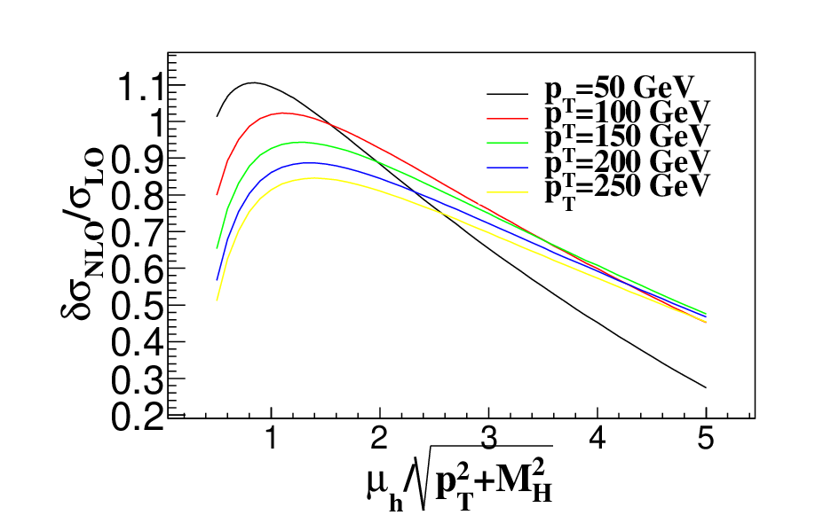
Figure 5: The NLO contribution of the hard function for different pTp_{T} cuts at the 88 TeV LHC.
Refer to caption
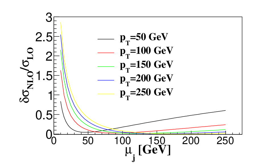
Figure 6: The NLO contribution of the jet function for different pTp_{T} cuts at the 88 TeV LHC.
Refer to caption
Figure 7: The NLO contribution of the soft function for different pTp_{T} cuts at the 88 TeV LHC.

In Fig. 5, we show the contribution to the NLO correction from only the hard function, normalized by the LO result, as a function of the hard scale. The hard function takes maximum values when the hard scale is around pT2+MH2\sqrt{p_{T}^{2}+M_{H}^{2}} for pT=100∼250p_{T}=100\sim 250 GeV. And the contributions from the hard function are very large, generally larger than 0.5 for pT=100∼250p_{T}=100\sim 250 GeV. This means that the hard function is very important, and needs to be calculated with higher precision. Resummation is a way to achieve this target. On the other hand, we also notice that the terms which can be resummed are only a limited part of the hard function. There is also significant contribution from those terms which are scale independent. Here, we choose 2.5​pT2+MH22.5\sqrt{p_{T}^{2}+M_{H}^{2}} as the default hard scale. The scale uncertainty of final resummed result from variation of the hard scale is about 12%12\%, as shown in Fig.  8.

In Fig. 6, we show the contribution to the NLO correction from only the jet function, normalized by the LO result, as a function of the jet scale. The jet function drops very quickly when the jet scale is smaller than 50 GeV, and changes very slowly when the jet scale is larger than 50 GeV. We can also see that the contribution from the jet function is about 10%10\% if pTp_{T} is larger than 100 GeV. The soft function has a similar behavior, as shown in Fig. 7, except that the contribution from the soft function is about 30%30\% if pTp_{T} is larger than 100 GeV. We choose μj≈150\mu_{j}\approx 150 GeV, μs≈100\mu_{s}\approx 100 GeV as the default jet and soft scales, respectively. The uncertainties of the final resummed result from the variation of jet and soft scales are about 2.4%2.4\% and 5.8%5.8\% as shown in Fig. 9 and Fig. 10, respectively.

Finally, to examine the factorization scale uncertainty in the final resummed result, we vary the factorization scale from MH/2M_{H}/2 to 2​MH2M_{H} and show the resummed result in Fig. 11. For comparation, we present scale uncertainties of the NLO result obtained by varying μ=μR=μf=MH\mu=\mu_{R}=\mu_{f}=M_{H} by a factor of 2, as done in Ref. [29]. After matching the resummed result with the NLO one, as shown in Eq. 89, the result is shown in Fig. 12. We see that both the resummed and matched results have smaller scale uncertainties than the NLO result.

Refer to caption
Figure 8: The hard scale uncertainty of the resummation results at the 88 TeV LHC.
Refer to caption
Figure 9: The jet scale uncertainty of the resummation results at the 88 TeV LHC.
Refer to caption
Figure 10: The soft scale uncertainty of the resummation results at the 88 TeV LHC.
Refer to caption
Figure 11: The scale uncertainty of the NNLL and NLO results for the Higgs boson and one jet aasociated production with large pTp_{T} at the 88 TeV LHC for gg channel.
Refer to caption
Figure 12: The scale uncertainty of the matched and NLO results for the Higgs boson and one jet associated production with large pTp_{T} at the 88 TeV LHC for the gg channel.

The case of g​qgq channel is similar to the g​ggg channel, and the scale uncertainty after resummation reduces more significantly compared with the g​ggg channel; see Figs. 13,14. For the q​q¯q\bar{q} channel, the contribution is very small. So we do not show its result individually.

Refer to caption
Figure 13: The scale uncertainty of the NNLL and NLO results for the Higgs boson and one jet associated production with large pTp_{T} at the 88 TeV LHC for gq channel.
Refer to caption
Figure 14: The scale uncertainty of the matched and NLO results for the Higgs boson and one jet associated production with large pTp_{T} at the 88 TeV LHC for the gq channel.
Refer to caption
Figure 15: The total scale uncertainty of the matched and NLO results for the single Higgs production with large pTp_{T} at the 88 TeV LHC.

Figure 15 shows the differential cross section as a function of pTp_{T} after matching to the NLO results. The result with resummation effects obviously reduces the large scale uncertainty compared to the NLO result. The ratio of the resummation result to the LO cross section is sensitive to pTp_{T}, changing from 1.8 to 1.0 as pTp_{T} varies from 100 to 290 GeV. The resummation results of the total cross section decrease the NLO one by about 11%11\% at the default scales when the Higgs boson pTp_{T} is larger than 100 GeV.

V.2 Discussion on the finite top quark mass effects

Up to now, the discussion is under the assumption of infinite top quark mass limit. However, in the case of large pTp_{T} Higgs boson production, the Higgs low energy theorem [63, 64] may fail to apply, and the top quark mass effects may make a sense. Considering the finite top quark mass will bring more complicated calculations, but also open a new way to probe the coupling of the Higgs to top quarks. When including the finite top quark mass, there exists only LO results [23, 24] and the corresponding parton shower effects [65, 32]. Unfortunately, there is no complete QCD NLO calculations of the Higgs plus jet including exact top mass effects. Only the subleading terms in 1/mt1/m_{t} have been calculated at QCD NLO [22, 30]. It is found that the infinite top quark mass limit is a very good approximation as long as pT<200p_{T}<200 GeV [21, 22]. Other discussions can been seen in Refs. [66, 67, 22]. We investigate the possible top quark mass effects by using the program HNNLO, presenting the results in Figs.16. For Higgs’s pTp_{T} less than 200200 GeV, the finite top quark mass effects are not obvious (the difference between the results with and without finite top quark mass is less than 4%4\%). For the pTp_{T} larger than 200200 GeV, the top quark mass begins to make sense and it is necessary to consider the finite top quark mass effects. We define the differential KK factor as

K⁡(pT)=d​σ∞N​L​O+N​N​L​Ld​σ∞L​O,K(p_{T})=\frac{d\sigma_{\infty}^{NLO+NNLL}}{d\sigma_{\infty}^{LO}}, (90)

where ∞\infty refers to the infinite top quark mass limit. Since the differential KK factor depends weakly on the top quark mass [68, 25, 69], we can obtain a reliable approximation of higher-order cross section by multiplying the KK factor to the exact top mass dependent LO one following the methods in Refs. [30, 70], which is given by

d​σd​pT=d​σmtL​Od​pT​K​(pT).\frac{d\sigma}{dp_{T}}=\frac{d\sigma_{m_{t}}^{LO}}{dp_{T}}K(p_{T}). (91)

Here, σmtL​O\sigma_{m_{t}}^{LO} means the exact LO cross section with finite top quark mass. The obtained pTp_{T} distribution of the Higgs boson at NNLL++NLO with finite top quark mass is shown in Fig. 16 as the black curve at the central value of the scales. In Fig. 16, we compare the resummation results with NLO ones in both cases of infinite and finite top quark mass.

Refer to caption
Figure 16: The central value (μF=MH,μh=2.5​pT2+MH2,μj=150​GeV,μs=100​GeV\mu_{F}=M_{H},\mu_{h}=2.5\sqrt{p_{T}^{2}+M_{H}^{2}},\mu_{j}=150~\rm{GeV},\mu_{s}=100~\rm{GeV})of four cases for the large pTp_{T} Higgs boson production at the 88 TeV LHC.The green curve is the NLO pTp_{T} distribution in the infinite top quark mass limit, the red curve is the NLO one with top mass effects, the blue curve is the NNLL++NLO one in the infinite top quark mass limit and the black curve is the NNLL++NLO with top quark mass effects.

These results can be used to improve the accuracy in probing the Higgs couplings to top quarks in the recent works [5, 6, 7].

V.3 Simple discussions on higher order corrections

After our paper appeared as an e-print, the authors in Ref. [71] investigated the same process and included the two-loop hard function. Their NNNLL results are not matched to the NNLO fixed order results in their paper. We use SCET to resum the large logarithm and match to the NLO fixed order one, while the authors in Ref. [71] use SCET to predict the approximated NNLO result, and their main conclusion is that the approximated NNLO correction increases the NLO by 50%50\%. The expanded NNLOp\rm{NNLO_{p}} results with the one-loop hard function squared (NNLO singular terms expanded from one-loop hard function, two-loop jet function, and two loop soft function) is shown in Fig. 17, and we see that the expanded NNLOp\rm{NNLO_{p}} result with the one loop hard function squared increases the NLO one significantly. The reason is that the main contribution to the two-loop hard function is from the squared one-loop hard function, shown as A02A_{0}^{2} term in B0B_{0} from Eq.(88). Besides, our results of LO and NLO singular terms are exactly the same as their results if we choose the same parameters as in [71].

Furthermore, we incorporate the two-loop hard function extracted from Refs.[53, 20], and find that the expanded NNLO results with two-loop hard function (NNLO singular terms from two-loop hard function, two-loop jet function and two-loop soft function) are numerically identical to the ones in Ref. [71] when the same parameters are chosen. The expanded NNLO result with two-loop hard function is shown in Fig. 17, where the term c2H−c1H2/2c_{2}^{H}-{c_{1}^{H}}^{2}/2 is added in order to compare with the expanded NNLOp\rm{NNLO_{p}} result with one-loop hard function squared. Figure 17 shows that the difference between the two kinds of expanded NNLO results is not very large. This is because the dominant contribution comes from the large logarithm terms which are obtained by expansion of the RG evolution expression, not the c2H−c1H2/2c_{2}^{H}-{c_{1}^{H}}^{2}/2. At NNLL order with the default scales, the contribution of negative logarithm terms in A0A_{0} dominates, and this leads to the fact that the resummation effects decrease the NLO cross section. After expanding the cross section to NNLO order, new positive logarithms, such as A02A_{0}^{2} terms in B0B_{0}, overwhelm the negative ones. Thus, the corrections for the two kinds of expanded NNLO results with the one-loop and two-loop hard function, respectively, become positive as shown in Fig.17, whether the c2H−c1H2/2c_{2}^{H}-{c_{1}^{H}}^{2}/2 term is included or not. The NNNLL resummation effect matched to NNLO fixed order deserves to be studied further, but is beyond the scope of this paper, and left for future work.

Refer to caption
Figure 17: The total scale uncertainties of the LO, NLO, expanded NLO, expanded NNLOp\rm{NNLO_{p}} (with one-loop hard function squared), and expanded NNLO (with the two-loop hard function ) results varying the scale from MH/2M_{H}/2 to 2​MH2M_{H} with all channels at the 88 TeV LHC.

VI Conclusion

We have studied the Higgs boson production at large pTp_{T} at the LHC, including the resummation effects in SCET. We find that the resummation effects decrease the NLO cross sections by about 11%11\% at the central values of the scales when the Higgs boson pTp_{T} is larger than 100100 GeV, and also reduce the scale uncertainty obviously. Moreover, we discuss the top mass effects numerically, and find that the top quark mass effects increase with the increasing of pTp_{T}. The pTp_{T} distribution of Higgs boson is important for describing the Higgs boson production at the LHC, and it is sensitive to the QCD higher order corrections. A precise measurement of the Higgs pTp_{T} is expected to be given in the near future and its precise prediction is very important for the experimental analyses. Thus, it is necessary to precisely investigate the large pTp_{T} behavior of the Higgs boson, and any deviation of the Higgs boson’s pTp_{T} distribution will give hints to the possible modification of the Higgs couplings to the top quark, which will shed light on the new physics.

Acknowledgements.
This work was partially supported by the National Natural Science Foundation of China, under Grants No. 11375013 and No. 11135003. Jian Wang was supported by the Cluster of Excellence Precision Physics, Fundamental Interactions and Structure of Matter (PRISMA-EXC 1098).

References

  • [1] S. Chatrchyan et al. (CMS Collaboration), Phys.Lett. B716, 30 (2012), eprint 1207.7235.
  • [2] G. Aad et al. (ATLAS Collaboration), Phys.Lett. B716, 1 (2012), eprint 1207.7214.
  • [3] S. Chatrchyan et al. (CMS Collaboration), JHEP 1305, 145 (2013), eprint 1303.0763.
  • [4] R. V. Harlander and T. Neumann, Phys.Rev. D88, 074015 (2013), eprint 1308.2225.
  • [5] A. Azatov and A. Paul, JHEP 1401, 014 (2014), eprint 1309.5273.
  • [6] A. Banfi, A. Martin, and V. Sanz, JHEP 1408, 053 (2014), eprint 1308.4771.
  • [7] C. Grojean, E. Salvioni, M. Schlaffer, and A. Weiler, JHEP 1405, 022 (2014), eprint 1312.3317.
  • [8] Tech. Rep. ATLAS-CONF-2014-011, CERN, Geneva (2014).
  • [9] D. de Florian, G. Ferrera, M. Grazzini, and D. Tommasini, JHEP 1111, 064 (2011), eprint 1109.2109.
  • [10] D. de Florian, A. Kulesza, and W. Vogelsang, JHEP 0602, 047 (2006), eprint hep-ph/0511205.
  • [11] X. Liu and F. Petriello, Phys.Rev. D87, 014018 (2013a), eprint 1210.1906.
  • [12] X. Liu and F. Petriello, Phys.Rev. D87, 094027 (2013b), eprint 1303.4405.
  • [13] R. Boughezal, X. Liu, F. Petriello, F. J. Tackmann, and J. R. Walsh, Phys.Rev. D89, 074044 (2014), eprint 1312.4535.
  • [14] T. T. Jouttenus, I. W. Stewart, F. J. Tackmann, and W. J. Waalewijn, Phys.Rev. D88, 054031 (2013), eprint 1302.0846.
  • [15] C. W. Bauer, S. Fleming, and M. E. Luke, Phys. Rev. D63, 014006 (2000), eprint hep-ph/0005275.
  • [16] C. W. Bauer, S. Fleming, D. Pirjol, and I. W. Stewart, Phys. Rev. D63, 114020 (2001), eprint hep-ph/0011336.
  • [17] C. W. Bauer and I. W. Stewart, Phys. Lett. B516, 134 (2001), eprint hep-ph/0107001.
  • [18] C. W. Bauer, D. Pirjol, and I. W. Stewart, Phys. Rev. D65, 054022 (2002), eprint hep-ph/0109045.
  • [19] T. Becher and M. Neubert, Phys. Rev. Lett. 97, 082001 (2006a), eprint hep-ph/0605050.
  • [20] T. Becher, G. Bell, C. Lorentzen, and S. Marti, JHEP 1402, 004 (2014a), eprint 1309.3245.
  • [21] V. Ravindran, J. Smith, and W. Van Neerven, Nucl.Phys. B634, 247 (2002), eprint hep-ph/0201114.
  • [22] R. V. Harlander, T. Neumann, K. J. Ozeren, and M. Wiesemann, JHEP 1208, 139 (2012), eprint 1206.0157.
  • [23] R. K. Ellis, I. Hinchliffe, M. Soldate, and J. van der Bij, Nucl.Phys. B297, 221 (1988).
  • [24] U. Baur and E. N. Glover, Nucl.Phys. B339, 38 (1990).
  • [25] R. V. Harlander and K. J. Ozeren, JHEP 0911, 088 (2009), eprint 0909.3420.
  • [26] C. R. Schmidt, Phys.Lett. B413, 391 (1997), eprint hep-ph/9707448.
  • [27] D. de Florian, M. Grazzini, and Z. Kunszt, Phys.Rev.Lett. 82, 5209 (1999), eprint hep-ph/9902483.
  • [28] C. J. Glosser and C. R. Schmidt, JHEP 0212, 016 (2002), eprint hep-ph/0209248.
  • [29] R. Boughezal, F. Caola, K. Melnikov, F. Petriello, and M. Schulze, JHEP 1306, 072 (2013), eprint 1302.6216.
  • [30] M. Grazzini and H. Sargsyan, JHEP 1309, 129 (2013), eprint 1306.4581.
  • [31] U. Langenegger, M. Spira, A. Starodumov, and P. Trueb, JHEP 0606, 035 (2006), eprint hep-ph/0604156.
  • [32] E. Bagnaschi, G. Degrassi, P. Slavich, and A. Vicini, JHEP 1202, 088 (2012), eprint 1111.2854.
  • [33] C. Arnesen, I. Z. Rothstein, and J. Zupan, Phys.Rev.Lett. 103, 151801 (2009), eprint 0809.1429.
  • [34] E. Laenen, G. Oderda, and G. Sterman, Phys. Lett. B438, 173 (1998), eprint hep-ph/9806467.
  • [35] M. Beneke, P. Falgari, and C. Schwinn, Nucl. Phys. B828, 69 (2010), eprint 0907.1443.
  • [36] T. Becher and M. D. Schwartz, JHEP 02, 040 (2010), eprint 0911.0681.
  • [37] J. C. Collins, D. E. Soper, and G. F. Sterman, Nucl.Phys. B250, 199 (1985).
  • [38] J. Collins, Cambrigde monographs on particle physics, nuclear physics and cosmology.32 (2011).
  • [39] P. Sun, C. P. Yuan, and F. Yuan (2014), eprint 1409.4121.
  • [40] A. V. Manohar, Phys. Rev. D68, 114019 (2003), eprint hep-ph/0309176.
  • [41] A. Idilbi and X.-d. Ji, Phys.Rev. D72, 054016 (2005), eprint hep-ph/0501006.
  • [42] V. Ahrens, A. Ferroglia, M. Neubert, B. D. Pecjak, and L. L. Yang, JHEP 1009, 097 (2010), eprint 1003.5827.
  • [43] T. Becher and M. Neubert, Phys. Rev. D79, 125004 (2009a), eprint 0904.1021.
  • [44] A. Ferroglia, M. Neubert, B. D. Pecjak, and L. L. Yang, Phys.Rev.Lett. 103, 201601 (2009a), eprint 0907.4791.
  • [45] A. Ferroglia, M. Neubert, B. D. Pecjak, and L. L. Yang, JHEP 0911, 062 (2009b), eprint 0908.3676.
  • [46] T. Becher and M. Neubert, Phys.Rev.Lett. 102, 162001 (2009b), eprint 0901.0722.
  • [47] T. Becher and M. Neubert, JHEP 0906, 081 (2009c), eprint 0903.1126.
  • [48] V. Ahrens, M. Neubert, and L. Vernazza, JHEP 1209, 138 (2012), eprint 1208.4847.
  • [49] G. Korchemsky and A. Radyushkin, Nucl.Phys. B283, 342 (1987).
  • [50] G. Korchemsky, Phys.Lett. B220, 629 (1989).
  • [51] I. Korchemskaya and G. Korchemsky, Physics Letters B 287, 169 (1992).
  • [52] T. Becher, M. Neubert, and B. D. Pecjak, JHEP 01, 076 (2007), eprint hep-ph/0607228.
  • [53] T. Gehrmann, M. Jaquier, E. Glover, and A. Koukoutsakis, JHEP 1202, 056 (2012), eprint 1112.3554.
  • [54] T. Becher and M. Neubert, Phys. Lett. B637, 251 (2006b), eprint hep-ph/0603140.
  • [55] T. Becher and G. Bell, Phys.Lett. B695, 252 (2011), eprint 1008.1936.
  • [56] T. Becher, M. Neubert, and G. Xu, JHEP 07, 030 (2008), eprint 0710.0680.
  • [57] T. Becher, G. Bell, and S. Marti, JHEP 1204, 034 (2012), eprint 1201.5572.
  • [58] T. Becher and M. D. Schwartz, JHEP 0807, 034 (2008), eprint 0803.0342.
  • [59] J. M. Campbell and R. Ellis, Nucl.Phys.Proc.Suppl. 205-206, 10 (2010), eprint 1007.3492.
  • [60] S. Catani and M. Grazzini, Phys.Rev.Lett. 98, 222002 (2007), eprint hep-ph/0703012.
  • [61] M. Grazzini, JHEP 0802, 043 (2008), eprint 0801.3232.
  • [62] M. Muether and CDF (Tevatron Electroweak Working Group, CDF Collaboration, D0 Collaboration) (2013), eprint 1305.3929.
  • [63] J. R. Ellis, M. K. Gaillard, and D. V. Nanopoulos, Nucl.Phys. B106, 292 (1976).
  • [64] M. A. Shifman, A. Vainshtein, M. Voloshin, and V. I. Zakharov, Sov.J.Nucl.Phys. 30, 711 (1979).
  • [65] J. Alwall, Q. Li, and F. Maltoni, Phys.Rev. D85, 014031 (2012), eprint 1110.1728.
  • [66] S. Dittmaier, S. Dittmaier, C. Mariotti, G. Passarino, R. Tanaka, et al. (2012), eprint 1201.3084.
  • [67] I. W. Stewart, F. J. Tackmann, J. R. Walsh and S. Zuberi, Phys. Rev. D 89, 054001 (2014),1307.1808.
  • [68] M. Spira, A. Djouadi, D. Graudenz, and P. Zerwas, Nucl.Phys. B453, 17 (1995), eprint hep-ph/9504378.
  • [69] A. Pak, M. Rogal, and M. Steinhauser, JHEP 1002, 025 (2010), eprint 0911.4662.
  • [70] J. Grigo, J. Hoff, K. Melnikov and M. Steinhauser, PoS RADCOR 2013, 006 (2013),1311.7425.
  • [71] T. Becher, G. Bell, C. Lorentzen and S. Marti, JHEP 1411, 026 (2014),1407.4111.