Effects of intrinsic noise on a cubic autocatalytic reaction diffusion system
Abstract
Starting from our recent chemical master equation derivation of the model of an autocatalytic reaction-diffusion chemical system with reactions and , , we determine the effects of intrinsic noise on the momentum-space behavior of its kinetic parameters and chemical concentrations. We demonstrate that the intrinsic noise induces molecular interaction processes with , where is the number of molecules participating of type or . The momentum dependences of the reaction rates are driven by the fact that the autocatalytic reaction (inelastic scattering) is renormalized through the existence of an arbitrary number of intermediate elastic scatterings, which can also be interpreted as the creation and subsequent decay of a three body composite state , where corresponds to the fields representing the densities of and . Finally, we discuss the difference between representing as a composite or an elementary particle (molecule) with its own kinetic parameters. In one dimension we find that while they show markedly different behavior in the short spatio-temporal scale, high momentum (UV) limit, they are formally equivalent in the large spatio-temporal scale, low momentum (IR) regime. On the other hand in two dimensions and greater, due to the effects of fluctuations, there is no way to experimentally distinguish between a fundamental and composite . Thus in this regime behave as an entity unto itself suggesting that it can be effectively treated as an independent chemical species.
pacs
82.40.Ck, 11.10.–z, 05.45.–a, 05.65.+bI Introduction
Reaction diffusion (RD) systems are a versatile class of models capable of encoding a variety of phenomena observed in Nature in areas encompassing physics, biology, ecology, chemistry and many other fields [1, 2, 3, 4]. Their application to chemical systems are of particular interest, as they include biologically relevant phenomena such as pattern formation and self-replication, and therefore can be used as proxies for high-level biological systems [5, 6]. While RD systems have been mostly studied from a deterministic standpoint, any faithful application to biological systems must take into account the effects of noise, since an important facet of such systems is its exchange of matter and energy with the environment; a process which clearly brings in some amount of stochasticity.
To reflect this, there have been recent efforts to study stochastic chemical reaction diffusion systems [7, 8, 9]. In particular, when such systems are coupled with external noise it is known that there are renormalization effects due to the fluctuations represented by the noise (by external we mean fluctuations that are not inherent to the chemistry itself). These affect for example, the strength of the chemical interactions that, in turn, induce new interactions not originally present in the “macro-level” chemistry [8]. However, independently of the above, there is also some form of intrinsic noise in the chemical system whose effects are less understood. Qualitatively, one can interpret this intrinsic noise as a manifestation of the underlying mechanisms that lead to the observed behavior of reaction diffusion systems at the level of their chemical kinetics. Because of this, it is important to understand the precise nature and effects of noise, as it might give intuition and provide hints for understanding the internal structure of the system [10].
In light of this, in this paper we seek to determine whether the inherent stochasticity in the nature of the chemical reactions themselves leads to effects similar to those induced by the external or noise. Of course this particular stochasticity is restricted by certain assumptions when we attempt to model these reactions in terms of kinetics. The most basic is that the molecules are random walkers in a -dimensional space that collisions between them occur as a function of the probability of encounters between these random walkers. Most collisions are elastic and do not result in a chemical reaction, whereas comparatively few are inelastic and lead to the actual chemistry that we are interested in. The relative scarcity of the latter with respect to the former implies that the chemically interesting inelastic collisions are effectively statistically independent and therefore the chemical reactions (occurring at large scales) are Markovian in nature. (Note that the assumption of the chemical reactions as a Markovian process is valid only up to a resolution limit which corresponds to the mean free path of the molecules involved in the reaction.)
In a previous paper [9] we considered as a test case a generic spatially extended set of macroscopic chemical reactions,
| (1) |
There is a cubic autocatalytic step for at rate , and decay reactions at rates that transform and into inert products and . Finally, is fed into the system at a rate and both and are allowed to diffuse with diffusion constants and respectively. We determined the form of the intrinsic noise associated with this system of reactions through a procedure which took us from the Master equation describing its chemistry (and that captures its Markovian nature) to an effective non–equilibrium field theory action (Cf. Appendix. A). This enabled us to derive a set of Langevin equations that incorporated the effects of the intrinsic noise. The structure of the noise was described through unique correlation functions. These required the existence of a collective mode where the are the fields encoding the chemical concentrations of the species.
In this sequel paper we focus on the effects of this noise. Specifically we seek to determine whether the physical parameters of the model inherit a scale-dependence as a function of the noise, and if so, whether this induces new interactions (relevant and irrelevant) apart from those initially present in the macroscopic chemistry specified by Eq. (1). We answer this question positively and consequently investigate the spatiotemporal scales at which these induced interactions manifest themselves along with the momentum space behavior of the parameters and chemical concentrations in the limiting regimes. To denote the limits we employ the field theory “jargon” whereby the large spatiotemporal scales corresponding to low wave-number and frequency are referred to collectively as the infrared (IR) regime, whereas the small spatiotemporal scales corresponding to high wave-number and frequency is the ultraviolet (UV) regime.
Since our goal is to determine the scaling behavior between the two limits, a natural way to proceed is to use a renormalization group approach [11, 12] on the many-body description of (1) that we studied in [9]. Interestingly, we find that the irreversibility of the reactions leads to a time-directionality associated with the Feynman diagrams describing the interactions. This in turn severely restricts the possible topologies of the graphs and allows us to carry out a systematic exact calculation to determine the effect of the noise.
We find that the strength of the coupling that regulates the autocatalytic part of the chemical reaction is renormalized due to the Markovian nature of the process. Specifically the chemically relevant inelastic collisions () proceed through an arbitrary intermediate number of elastic collisions () modifying the coupling strength as we change scales. This scale dependence manifests itself only up to a critical dimension , above which (in the absence of cutoffs) the coupling constant is formally zero in the IR. Thus beyond the system must be considered an effective field theory, whose parameters must be determined by low momentum experiments. The number of parameters of this effective theory are most easily described in terms of recasting it via composite fields for the concentrations , and . In particular the reaction is then interpreted as proceeding through the formation of an intermediate state that was also essential in determining the Langevin equations for (1) that were derived in [9].
When probing the system at short spatiotemporal (UV) scales it turns out that there are two separate manifestations of (i) a composite bound state or (ii) an elementary particle (molecule) with its own bare kinetic terms each leading to different equations of motion. However, starting from both versions of leads to the same equations of motion. The physical implication of this is that one cannot experimentally resolve into its constituents and that it behaves as an elementary particle. In order to see its composite nature one would need to probe at spatio-temporal scales shorter than that associated with the mean free path of the chemicals. However in this limit the Markovian assumption is violated and new physics is required to describe the chemistry.
The fluctuations also lead to relevant new noise-induced interactions of the form for where is the number of molecules entering or leaving the reaction zone. Although all these higher order processes are naively divergent, to regulate them, one might think that an infinite number of “counter terms” need to be added. In two dimensions, however, it turns out that by again introducing composite concentration fields for the di-molecules and , the divergences in these induced interactions can be regulated by introducing just two new effective field theory parameters: the decay rates (masses) for and . Finally in three dimensions no new parameters are needed, however the equations of motion are modified: in order to describe the infrared physical chemistry at small momentum one needs to introduce higher order kinetic terms into the action for .
II Momentum-dependent reaction rate
In order to uncover the momentum scale behavior of the constituents of the model, we will resort to the many body description of Eq. (1). In this description the reaction is interpreted in terms of a three body inelastic collision where two particles of and one of are destroyed at an interaction vertex to create three of . When one writes down the master equation describing this reaction (see Eq. (49)), one finds that in order to conserve probabilities, it is also necessary to include the elastic collision . A graphical representation of this is shown in in Fig. 1, where the inelastic scattering is proportional to , while the elastic scattering is proportional to . Following this, the Doi-Peliti operator technique [13, 14] is used to write down an equivalent non-equilibrium field theory action [15, 16, 17] thus,
| (2) | |||||
where the ’s are fields representing the concentrations of the chemicals. (An outline of this method is shown in Appendix A, see [9] for more extensive details of the derivation.)

Since the action must be dimensionless, if we introduce a momentum scale along with the diffusive temporal scaling , it is straightforward to see that we have associated scaling dimensions:
| (3) |
where the starred fields are chosen to be dimensionless by convention and , where is the critical dimension (i.e. the dimension below which has non-vanishing finite value in the high-momentum UV limit). Generalizing the cubic interaction in (2) to the form , the general form of the critical dimension is seen to be which in this case (where ) implies that . Consequently the dimensionless version of the coupling constant is therefore the combination .
It is worth noting that the action shown in (2) corresponds to a “symmetric” phase in the sense that it possesses a symmetry due to particle number conservation (essentially equivalent to a form of the classic Lavoisier’s principle). The graphs that contribute to one particle irreducible vertex process or any intermediate state, must be constructed from the (directed) basic interactions shown in Fig. 1. The symmetry of the basic process corresponding to the inelastic chemical reaction (as well as the corresponding elastic reaction ), along with the unidirectionality of the reactions (being non-reversible) severely restrict the set of graphs that can be constructed. In fact looking at the topological structure of the bare vertices in Fig. 1, it becomes clear that there is no combination that can generate any diagram contributing to corrections to the propagator (), since this requires (graphically) one incoming and one outgoing line. This implies in turn that there is no momentum dependence of the diffusion constants or the decay terms .
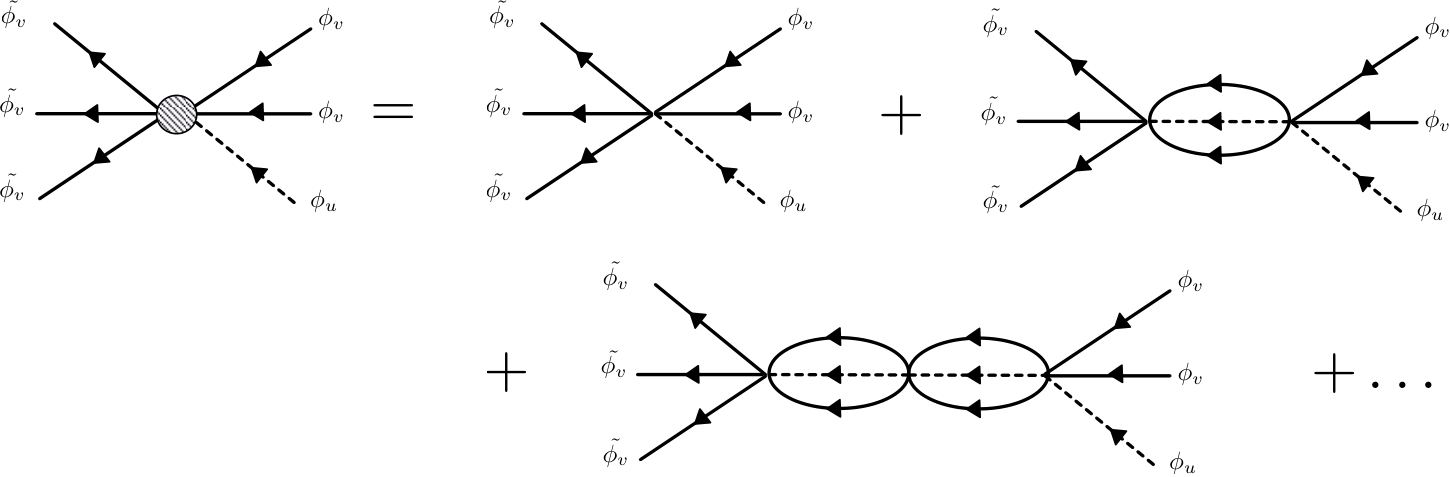
On the other hand, as shown in Fig. 2, it is clearly possible to rewrite the bare three body interaction in terms of a diagrammatic expansion corresponding to a perturbation series in . Each component in the expansion corresponds to an elastic re-scattering represented through a loop (the subscript 2 reflects the fact that the elastic re-scattering consists of two loops). Mathematically this is expressed through the vertex function (where the 3 refers to the number of incoming and outgoing lines in Fig. 1) whose formal expression is
| (4) | |||||
where the subscript i refers to inelastic. (The vertex function for elastic scattering is just -.)
Assuming there is an external momentum flowing into the graph from the three external legs, the explicit expression for the loop is,
| (5) | |||||
Through appropriate linear transformations and (legal) shifts of the momentum variables, it is easily shown that
| (6) |
where to avoid clutter we use the abbreviations and . Taking the Laplace transform of (4) renders it into a geometric sum via the convolution theorem and yields,
| (7) |
where is the Euler-Gamma function and . From (7) it is clear that is the reaction rate in the absence of fluctuations (since in that case , whereas the full expression reflects its function on the energy and momentum scale at which it is measured. It is therefore interpreted as the dimension-full running reaction rate.
The fluctuation term has a pole in one dimension and in every positive integer dimension. For physical reasons we restrict ourselves to the range and therefore we expose the relevant divergences through the identity , to rewrite
| (8) |
In order to carry out the corresponding renormalization—as in standard quantum field theory—it is convenient to introduce a dimensionless counterpart to . As mentioned before the dimensionless bare reaction rate in the presence of a momentum scale is . However, in order to simplify the algebra we will instead find it convenient to work with a slightly modified form thus
| (9) |
in terms of which the dimensionless running reaction rate is modified to
| (10) | |||||
By itself, this does not seem particularly useful, since we need to translate this into a physically measurable quantity. To do so we begin by defining a renormalized coupling constant at the convenient renormalization point .
Physically, this implies that we measure (experimentally) the coupling at and use it to determine what value of the bare dimensionless coupling corresponds to the physically measured running . Of course, once this measurement is made, the value of the coupling at any other momentum scale is determined.
For this choice of measurement scale the connection between and simplifies to
| (11) |
with given by Eq. (9). Finally, combining Eqns. (10) and (11), the expression for the (running) coupling constant for arbitrary momentum and energy scale is
and of course by inspection, it is apparent that at the renormalization point one obtains the equivalence as should be the case by definition.
We see that for the coupling in Eq. (10) is finite in both the UV and IR regimes and as we get . At the critical dimension we can expand the denominator in a power-series to get
| (13) |
which suggests that there is a Landau pole at . A similar situation is found in quantum electrodynamics where such a singularity is what leads to the divergence of the bare charge in the UV limit. Correspondingly, this is interpreted as the harbinger of phenomena or degrees of freedom in the UV or, equivalently, at the shorter length scales, and which in a chemical context hints at the presence of short lived or intermediate substances in the mechanism of the original chemical reaction.
A naive use of this dimensionally regulated answer yields as the result
| (14) |
implying that the coupling goes to zero in the continuum limit. This can also be seen through the associated function for which has the particularly simple form,
| (15) | |||||
This has two fixed points: a trivial one at and a non-trivial one at . Note that the non-trivial fixed point exists only when or . In the former case is IR stable while is UV stable, with the situation being reversed in the latter case. On the other hand when and there is only a single fixed point which is IR stable but UV divergent (see Fig. 3).
Taken naively this seems to indicate that there is no momentum dependence of the coupling once we are beyond one dimension. In reality, however, there is a characteristic length scale in the system. Indeed, as discussed in the introduction, beneath the development of the master equation and its corresponding action (2) lurks the assumption of a lattice on which the chemicals hop between sites. In addition, the size of the lattice must be larger than the mean free path of each chemical species in order to preserve the Markovian nature of the collisions. In other words the term in (14) really indicates a cut-off of the form , where is the maximum limit of the lattice momentum. Therefore in two dimensions, the action (2) represents an effective field theory with an UV cutoff.
In three dimensions we get the dimensionally regulated answer:
| (16) |
which suffers from the same pathologies as in the two-dimensional case.
In order to obtain the correct effective theory, we make use of auxiliary fields that allows us to interpret the sum of loops in the vertex function (i.e. the sum of elastic scatterings) as going through a single composite state . We can imagine the field as representing the density of a “cloud” of chemicals involved in the elastic scattering. This field then requires a “mass” (decay rate) and wave-function renormalization to render the system finite. The effective theory can then be described in terms of some low energy parameters such as long distance reaction rates, as well as the low momentum decay rates of composite fields. As is well known, this can be made explicit by making use of the well known technique of the Hubbard-Stratonovich [18, 19] transformation, which we describe and apply next to this problem.
III Composite field operators
We now introduce the composite fields and into the previous field theory via a Hubbard-Stratonovich transformation and discuss the differences between an “elementary” field and a composite one. We will find that at large times and distances, these two theories are indistinguishable. However at short scales (high momentum), these theories differ for .
Our starting point, once again, is the unshifted action (2)
| (17) | |||||
To carry out the Hubbard-Stratonovich transformation, we construct a second action which defines the composite fields and thus,
| (18) | |||||
and add it to obtaining,
| (19) | |||||
Eliminating the constraint equation defining leads back to the original equation of motion for the fields . From (19), it is apparent that while the composite field is formed through a combination of a single and two ’s, it has two potential decay channels (i) it converts into either 3 ’s or (ii) back again to the original constituents, a single and two ’s (Cf. Fig. 4).
It is instructive to perform a comparison of the above, with the case where we consider as an elementary scalar particle. In this version, instead of the local interaction found in there is a fundamental (or rather bare) kinetic energy term for the field, as well as an unrenormalized decay rate . To keep the dimensionality of the elementary the same as in the composite case, the “free” part of the field action needs to be divided by . Consequently, the action is now
| (20) | |||||
Note that in the models defined by either (19) or (20), the structure of the Schwinger-Dyson equations are quite similar.
Having introduced , the process of elastic scattering is now interpreted as proceeding through the exchange of a composite field. This involves the composite propagator, whose inverse is given by the dimensionally regulated expression
| (21) | |||||
In the case where is an elementary particle, this is instead
| (22) | |||||
where for the sake of simplicity we have chosen the same diffusion constant for the free part as in the induced one, i.e. .
To complete the renormalization procedure in terms of the composite field we must now allow for “wave function” renormalization for the field as well as “mass” (decay rate) renormalization. Since the vertex function depends on the combination , the inverse propagator (21) can therefore be expanded in a power series in thus
where can be thought of as a self-energy function. The expansion for the elementary is identical, with the exception that the first term in () i.e , is replaced by . Otherwise the renormalization procedure is identical in both cases. Let us first consider the situation for .
III.1 One and two dimensions
For both the composite and elementary ’s we can rewrite in the form
| (24) |
for and the quantities and are obtained from the first two terms in the expansion of Eq. (). (We will henceforth drop the subscript for and unless mentioned otherwise it refers to both the elementary and composite versions of the model.) The subscript refers to the subtraction of the first two terms in the power series (), is the renormalized decay rate for the field and is the wave function renormalization. Note that at low momentum, apart from the rescaling by , the inverse propagator resembles the free field one.
When is composite this leads to the identities
| (25) |
whereas when it is considered elementary we have,
| (26) |
Next we introduce the renormalized vertex for making use of the identities
| (27) |
where is the renormalized propagator for . Consequently the combination
| (28) |
is invariant under renormalization. Combining these leads us to a finite expression for the running reaction rate thus
| (29) |
In two dimensions is just zero and therefore this reduces to
| (30) |
In particular using (28) and the definition of we have that
| (31) |
Finally, employing Eqns. (25) or (26) allows us to relate to .
We thus conclude that in , the renormalized coupling is proportional to through the wave function renormalization term . This suggests that when we use actual cutoffs to regulate the integrals, the renormalized coupling is related to the inverse of the physical cutoff of the problem. This confirms our previous intuition that the system can only be described by an effective field theory with a momentum space (or spatial) cutoff. It is also apparent that there is no difference between a fundamental or composite at this level in either the IR or UV limits. The dependence on the parameter can be eliminated by evaluating the running coupling constant (momentum dependent reaction rate) at a particular reference point . In terms of this reference point (as chosen for Eq. (11)) one finds the reaction rate is given by
| (32) |
thus explicitly showing that can be replaced by the physical quantity .
Moving onto one dimension which is the critical dimension, from Eqns. (25) and (26) we find that the wave function renormalization is finite. Thus only mass renormalization is needed which can again be translated into defining at a particular reference value . In this case the second term in () is
| (33) |
which leads to
| (34) |
Once again making use of (27) we find that and therefore the terms linear in cancel. Thus the renormalized propagator for the composite is
| (35) |
Once again the parameter can be eliminated by defining at some scale such that
| (36) |
implying that it goes to zero as in the UV limit. Note that this is equivalent to our previous result Eq. (13).
Through a similar sequence of manipulations it can be shown that for the elementary we have the relation
| (37) |
and therefore this is equivalent to the composite only when in which case (the standard “compositeness” condition in field theory). The corresponding analog to Eq. (36) is
| (38) |
where . Here, the running coupling goes to zero linearly with as opposed to logarithmically. Thus unlike in the two dimensional case there is a difference between the elementary and composite manifestations of .
III.2 Higher dimensions
The renormalization process for requires the introduction of higher derivative terms into the effective action for the field . This is due to the fact that the self-energy function in () has an increasing number of divergent terms.
In one and two dimensions, as discussed previously, the first two terms in the series diverge and are regulated via decay rate and wave function renormalization respectively. Starting from one begins to induce terms that are not originally present in Eqns. (19) and (20). Consequently one needs to subtract three terms from to obtain a finite contribution. (And four in and so on.) The resulting renormalized propagator can be written as
| (39) |
where the term corresponds to the addition of a new induced term that needs to be inserted in (19) and (20). This term has the form
| (40) |

IV Fluctuation Induced Processes
The interactions shown in Fig. (1) are such that they can induce processes (via fluctuations) that are not explicitly present in the original action described by Eq. (2) . (For examples of this phenomenon in out of equilibrium RD systems, but generated by noise, cf. Ref. [8].) While this is not problematic if the induced terms are , a serious problem appears if the terms bring with them a divergence. If each order in perturbation theory leads to new interactions which are divergent, then usually an infinite number of parameters are needed to define the theory. In such a situation physical predictions cannot be made as they depend on an arbitrary number of parameters. In that case the theory is called non-renormalizable. Although we will find that indeed there are an infinite number of induced processes that appear superficially divergent, by an appropriate introduction of composite field operators, we will find that only three long distance (infrared) parameters will be needed to describe all the induced processes.
The induced processes in this case can be constructed from diagrams that represent scattering for for both elastic and inelastic processes. An example of this for for the inelastic case is given in Fig. 5 where we consider the diagrams for in (a) and in (b). Although at first sight it appears these diagrams are naively divergent, if one thinks of them as proceeding through “tree level” diagrams in terms of the production of di-molecule and tri-molecule states, then the only renormalizations necessary are those of the tri-molecule propagator as well as decay constant renormalization for the di-molecule correlation functions. In terms of the renormalized parameters of the propagator and di-molecule propagators, these induced processes are then rendered finite.
Going back to Fig. 5a,b, we see the formation of a single loop which now consists of two ’s (or, equivalently, a correlation function for the composite field ). If we instead considered the process (c) this would have been facilitated instead by the correlation function for the composite field . In terms of the composite fields, these processes are “tree graphs” in the Green’s functions for , and . These internal processes are reversible in that and etc. Starting at we can have both the and correlation functions occurring in the composite field “tree” diagram as shown in (d) for the process .
To expose and study the divergence structure of the correlation functions, we only need to calculate a single loop (unlike for the case of the elementary correlation function which is a geometric sum of two loop graphs). We will assume that an external momentum flows into the right-most vertices in Fig. 5 and to simplify the discussion we will set the energy and momentum of the “new” incoming and outgoing particles (beyond the basic reaction) to zero. We will then only have to consider the internal one loop graphs at some arbitrary momentum . The expression for the one loop integral is given by,
| (41) | |||||
This can be calculated exactly and after Laplace transforming to –space one gets,
| (42) |
where now
| (43) |
Note that for the single loop the critical dimension is now , and therefore . At , and we get the finite result:
| (44) |
so that this process vanishes as for large momenta.
To evaluate in the critical dimension , we exponentiate the term in above and expand the exponential thus,
| (45) | |||||
Inserting the result of this expansion back into (42), we immediately see that the only term that diverges as is the first term in the expansion. In order to regulate this divergence we only need to renormalize the decay rate or so-called “Mass” renormalization.
We start by assuming that the one-loop integral corresponds to the correlation function for the composite field . Next identifying the zero energy-momentum piece of the dimensionless propagator as we get
| (46) |
Consequently the renormalized version of the correlation function is now
| (47) |
where .
Thus in two dimensions, all processes are rendered finite by the introduction of only two new parameters corresponding to the decay rates for the two composite fields and . In terms of these two parameters (and the renormalized coupling ) all the induced couplings can be determined.
Finally, the full expression for the Laplace transform of the vertex function of Fig. 5a is just , where at we need to replace by the regulated . It is not hard to see that for processes like Fig. 5b and extensions to the form this generalizes to
| (48) |
V Conclusions
In this paper we presented a detailed analysis of the effects of intrinsic noise on a spatially extended reaction-diffusion chemical model (1). We found that remarkably, the short distance behavior of the system could be determined analytically by studying the model in the symmetric phase of the field theory [9] corresponding to the chemical reactions described by Eq. (1). The symmetric phase of the field theory reflects particle number conservation and consequently the only allowed graphs in its Feynman diagram representation are for , with . The fluctuations due to the intrinsic noise leads to two types of potentially divergent graphs in the theory. The first divergent graph, is a 2-loop graph which first diverges in the critical dimension . This graph we relate to the renormalization of the reaction rate. The second class of divergent graphs first appear in in the induced processes. These we regulate using the standard technique of dimensional regularization. We then investigated what (if any) are the new low energy (large spatio-temporal) parameters that need to be specified to define the correct finite and renormalized theory which includes the effects of the fluctuations.
We find that one parameter is the critical dimension for the behavior of the reaction rate parameter , which happens to be . This reaction rate gets renormalized through a sequence of elastic collisions (two-loop graphs) that occur between the chemically relevant inelastic collision. As a result, it acquires a momentum dependence, which in the critical dimension we can specify by determining the reaction rate at late times. Equivalently, this is also determined by representing the elastic collisions as a composite three body state , and then determining its rate of decay. We also find that in it is possible to distinguish between the situations where is a bonafide composite state and the case where instead, it is an elementary chemical with its own kinetic energy and decay terms. This is done by investigating the large momentum (short distance) behavior of the momentum dependent reaction rate. The decay rate in the version with an elementary goes to zero in the high momentum UV limit faster than in the case where is composite. The point where the wave function renormalization of the elementary goes to zero, is where the two versions of the model are identical.
Starting in two dimensions, two new parameters are needed to describe the system. These can be thought of as being the decay rates (masses) for the composite systems and . To obtain these parameters one would need to experimentally measure the reaction rates for two inelastic reactions such as and . Once that is done, all the induced reaction rates can be calculated. The renormalized equation for the field in two dimensions includes an induced free field kinetic term. In 3 dimensions the fluctuations have a further effect of changing the renormalized equation for the field to one having higher spatio-temporal derivatives. Thus in terms of the running coupling constant as well as two measurable induced coupling constants, we have determined the effective field theory which results from the intrinsic noise inherent in this chemical reaction diffusion model.
We did not discuss the infrared properties of the theory with broken symmetry, which is the sector that relates directly to the chemistry. To do so, one would follow a two step approach. First, one needs to determine the classical densities as a function of time and the classical response function which depends on both momentum and time. Then we would make use of the running coupling constant found in this paper to determine the asymptotic behavior of the momentum dependent densities including fluctuations by solving the Callan-Symanzik equation [21, 22]. This approach is worked out in detail for the example of the process in [11] and extends the arguments standard in relativistic quantum field theory to this class of non-equilibrium models.
Appendix A Chemical master equation and many body formalism
In order to develop the master equation formalism for our system of chemical reactions (1), we first divide the space in which the reactions take place into a dimensional hyper-cubic lattice of cells and assume that we can treat each cell as a coherent entity. We assume the interactions occur locally at a single cell site and that there is also diffusion modeled as hopping between nearest neighbors. Assuming that the underlying processes are Markovian, they can be described by a probability distribution function which gives the probability to find the particle configuration at time . Here is a vector composition variable where represents the number of molecules of a species at site . Following standard methods, one obtains for the master equation for the chemical reactions in (1) including diffusion
| (49) | |||||
where is the characteristic length of the cell and denotes the sum over nearest neighbors.
The master equation (49) along with the sextic interaction shown in Fig. 1 lends itself to a many body description [13], accomplished by the introduction of an occupation number algebra with annihilation/creation operators for and for at each site . These operators obey the Bosonic commutation relations
| (50) |
and define the occupation number operators and satisfying the following eigenvalue equations:
| (51) |
We next construct the state vector
| (52) | |||||
which upon differentiating with respect to time , can be written in the suggestive form
| (53) |
resembling the Schrödinger equation. Finally, taking the time derivative of Eq. (52) and comparing terms with the Hamiltonian in (53) we make the identification
| (54) | |||||
Having defined the space, the appropriate wave function and the Hamiltonian, we next seek to evaluate the operator using the path integral formulation. Following the standard procedure for obtaining the coherent state path integral [15, 12, 16] to the GS system, letting the coherent state (related to the operator ) represent and (related to the operator ) represent we obtain
| (55) |
where the action is given by
| (56) | |||||
This is Eq. (2) in the body of the text.
References
- [1] M. Cross and H. Greenside, Pattern Formation and Dynamics in Nonequilibrium Systems (Cambridge Univ. Press, Cambridge, 2009).
- [2] D. Walgraef, Spatio-Temporal Pattern Formation (Springer, New York, 1997).
- [3] A. S. Mikhailov, Foundations of Synergetics I, 2 ed. (Springer, Berlin, 1994).
- [4] B. A. Grzybowski, Chemistry in Motion: Reaction-Diffusion Systems for Micro- and Nanotechnology (Wiley, Chichester, 2009).
- [5] J. E. Pearson, Science 261, 189 (1993).
- [6] K.-J. Lee, W. D. McCormick, J. E. Pearson, and H. L. Swinney, Nature 369, 215 (1994).
- [7] F. Lesmes, D. Hochberg, F. Morán, and J. Pérez-Mercader, Phys. Rev. Lett. 91, 238301 (2003).
- [8] D. Hochberg, F. Lesmes, F. Moran, and J. Pérez-Mercader, Phys. Rev. E. 68, 066114 (2003).
- [9] F. Cooper, G. Ghoshal, and J. Pérez-Mercader, Phys. Rev. E 88, 042926 (2013).
- [10] F. Cooper, G. Ghoshal, A. Pawling, and J. Pérez-Mercader, Phys. Rev. Lett. 111, 044101 (2013).
- [11] B. P. Vollmayr-Lee, J. Phys. A: Math. Gen. 27, 2633 (1994).
- [12] U. C. Täuber, M. Howard, and B. P. Vollmayr-Lee, J. Phys. A: Math. Gen. 38, R79 (2005).
- [13] M. Doi, J. Phys. A: Math. Gen. 9, 1465 (1976).
- [14] P. Grassberger and M. Scheunert, Fortschritte der Physik 28, 547 (1980).
- [15] J. W. Negele and H. Orland, Quantum Many-Particle Systems (Perseus Publishing, Cambridge, 1998).
- [16] U. C. Täuber, in Aging and the Glass Transition, Vol. 716 of Springer Lecture Notes in Physics, edited by M. Henkel, M. Pleimling, and R. Sanctuary (Springer-Verlag, Berlin, 2007), pp. 295–348.
- [17] M.-P. Zorzano, D. Hochberg, and F. Moran, Phys. Rev. E 74, 057102 (2006).
- [18] R. Stratonovich, Doklady 2, 416 (1958).
- [19] J. Hubbard, Phys. Rev. Lett. 3, 77 (1959).
- [20] M. Gell-Mann and F. Low, Phys. Rev. 84, 350 (1951).
- [21] C. G. Callan, Phys. Rev. D 2, 1541 (1970).
- [22] K. Symanzik, Commun. Math. Phys. 18, 227 (1970).