Dynamic many-body theory:
Dynamic structure factor of two-dimensional liquid 4He
Abstract
We calculate the dynamic structure function of two-dimensional liquid 4He at zero temperature employing a quantitative multi-particle fluctuations approach up to infinite order. We observe a behavior that is qualitatively similar to the phonon-maxon-roton-curve in 3D, including a Pitaevskii plateau (L. P. Pitaevskii, Sov. Phys. JETP 9, 830 (1959)). Slightly below the liquid-solid phase transition, a second weak roton-like excitation evolves below the plateau.
Keywords:
Helium-II films, Phonon-Roton spectrum, Multi-particle fluctuationspacs
67.30.em, 67.30.H, 67.10.-jI Introduction
The static and dynamic structure of few-layer films of liquid helium absorbed on solid substrates at low temperatures has been studied experimentally, e.g. within neutron scattering measurements [1, 2, 3, 4], and theoretically [5, 6, 7, 8, 9, 10, 11, 12]. The earliest investigations of excitations [5, 6, 7, 8, 11] were based on generalizations of Feynman’s theory of excitations in the bulk liquid [13] and therefore only qualitative. Later work [10, 12, 14] employed correlated basis functions (CBF) theory [15, 16, 17]. These methods are simple enough for the application to non-uniform geometries including the inhomogeneity of the substrates and the non-trivial density profile of the films. Agreement with measurements of the dynamic structure was either semi-quantitative, or required some phenomenological input for a quantitative description of the various excitation types seen in the experiments [18] such as “layer-phonons”, “layer-rotons”, or “ripplons”.
Since then the development of theoretical tools for describing the dynamics of bulk quantum liquids has made significant progress, providing a quantitative description in the experimentally accessible density range for low and intermediate momenta, probing the short-range structure of the system [19, 20, 21, 22]. Due to the increasingly complicated form of more elaborate methods, application to inhomogeneous geometries is less straightforward. Building on the success of our method for both bulk 4He [23] and 3He [21, 22, 24], we here investigate mono-layer films of 4He which can be treated as strictly two-dimensional liquids.
Recently, novel numerical methods [25, 26, 27] have appeared that give access to dynamic properties of quantum fluids. These are algorithmically very important developments that will ultimately aide in the demanding elimination of background and multiple-scattering events from the raw data. However, it is generally agreed upon that the model of static pair potentials like the Aziz interaction describes the helium liquids accurately. Hence, given sufficiently elaborate algorithms and sufficient computing power, such calculations must reproduce the experimental data. The aim of our work is somewhat different: The identification of physical effects like phonon-phonon, phonon-roton, roton-roton, maxon-roton … couplings that lead to observable features in the dynamic structure function is, from simulation data, only possible a-posteriori whereas the semi-analytic methods pursued here permit a direct identification of these effects, their physical mechanisms, and their relationship to the ground state structure directly from the theory.
II Theoretical framework
The behavior of identical, non-relativistic particles in an external field , interacting via a pair potential , is governed by a microscopic Hamiltonian
| (1) |
The ground state is written in the Feenberg form [28]
| (2) |
where is a non- or weakly-interacting model wave function containing the appropriate symmetry and statistics of the system, and
| (3) |
is the correlation operator consisting of -particle correlation functions .
For homogeneous Bose systems such as three- and two-dimensional 4He, can be chosen to be 1 and the wave function (2,3) is in principle exact. The empirical Aziz potential [29] as interaction between the helium atoms has turned out to lead to results in quantitative agreement with experiments, see Ref. 30 for a review. With minimal phenomenological input, the same accuracy can be obtained with integral equation methods [31, 32]. In that case, the correlation functions are optimized by minimizing the ground state energy , viz.
| (4) |
Dynamics is treated along basically the same lines. In the presence of a time-dependent external perturbation
| (5) |
the time-dependent generalization of the ground state wave function (2) is
| (6) |
where
| (7) |
is the complex excitation operator. Its components, the fluctuations of the correlation functions, are determined by the least action principle [33, 34]
| (8) |
which generalizes the Euler-Lagrange Eq. (4) to the time-dependent case.
III Multi-particle fluctuations and density-density response
For weak external perturbations, the relationship between the perturbing external field and the induced density fluctuation
| (9) |
is linear and defines the density-density response function . In homogeneous, isotropic geometries where the ground state density is constant, the density-density response function is most conveniently formulated in momentum and energy space and defines the dynamic structure function
| (10) |
spelled out here for zero temperature and consequently .
The truncation of the sum of many-particle fluctuations (7) defines the level of our treatment of the dynamics. For example, the single-particle approximation
| (11) |
for the fluctuations leads to the time-honored Feynman dispersion relation [13]
| (12) |
Here, is the static structure function which can be obtained from experiments or ground state calculations. In this approximation, is described by a single mode located at the Feynman spectrum.
The importance of including at least two-particle fluctuations was first pointed out by Feynman and Cohen in their seminal work on “backflow” correlations [35]. A somewhat more formal approach was taken by Feenberg and collaborators who derived a Brillouin-Wigner perturbation theory in a basis of correlated wave functions [15, 16, 36, 37, 17]. These approaches determine, rigorously speaking, only the energy of the lowest-lying mode. The equations of motion method (8) employed here provides access to the full density-density response function
| (13) |
where is the phonon self-energy. In practically all applications, the excitation operator (7) has been truncated at the two-body level and the convolution approximation was used [38, 31] which is simple enough to be employed in non-uniform geometries [12, 18]. Then, the self-energy has the form
| (14) |
where is the dimension of the system. The three-body vertex describes the decay of a density fluctuation with wave vector into two waves with wave vectors and . It can be calculated in terms of ground state quantities, its general form is [39]
| (15) |
where is the “direct correlation function” and is the irreducible part of the three-body distribution function, see appendix B.
The lowest excitation branch is obtained by solving
| (16) |
When consistent approximations are used, the solution of Eq. (16) is identical to what was obtained by CBF perturbation theory.
Eqs. (13), (14) and (15) give the correct physics up to and somewhat beyond the roton minimum, the solution of Eqs. (14), (16) bridges about about 80 percent of the discrepancy between the Feynman spectrum and the experiment. The most prominent shortcoming of the approximation is that it misses the energy of the plateau. The reason for this shortcoming is that the energy denominator in the self-energy (14) contains the Feynman energies.
There are several ways to improve upon this: Brillouin-Wigner perturbation theory has been worked out by Lee and Lee [37] up to fourth order from which the general scheme can be seen. Some low-order processes contributing to the self-consistent self-energy are shown in Fig. 1.


Unfortunately that work did not utilize the fact that the ground state should be optimized and, therefore, obtained also spurious diagrams. The most complete derivation within the equations of motion scheme includes time-dependent triplet correlations [19, 20]. The theory reproduces, for the lowest mode, the first diagrams of CBF perturbation theory. The expected result is that the self-energy in Eq. (14) should be replaced by the self-consistent form
| (17) |
which leads to quantitative agreement between the theoretical excitation spectrum and the experimental phonon-roton spectrum. It still contains the Feynman energy as argument which should also be calculated self-consistently. We have simplified this part of the calculation by using the calculated phonon-roton spectrum in the energy arguments of the self-energy. This provides a slight improvement of the description in the momentum regime of the plateau.
IV Dynamic structure function of two-dimensional 4He
The only quantity needed for the calculation of the self-energy is the ground state distribution function and/or the static structure function . These quantities have been calculated in the past and are available in pedagogical and review-type literature, see Refs. 30, 40. We have here used the HNC-EL method including four and five-body elementary diagrams and triplet correlation functions as described in Ref. 32.
We have calculated the dynamic structure function in the regime between the equilibrium density of the system of Å-2 and the solidification density of Å-2 [30] in steps of Å-2. Compared to earlier work we have used an improved method for calculating the three-body vertex as described in appendix B. This leads to a slight lowering of the roton minimum by about K depending on density but to no qualitative changes. An overview of our results for the dynamic structure function is shown in Figs. 2 for four densities. In these figures, we also compare with the simulation data, including error bars, of Ref. 41.


Conventionally, one looks at the phonon-roton spectrum as the main feature of the excitations in the helium liquids. The phonon-roton spectra are shown, as a function of density, in Fig. 3.

These spectra display, apart from an energy and momentum scale which is distinctly different from the three-dimensional case, similarities to the 3D spectra: with increasing density, the roton energy is lowered, and the roton wave number becomes larger. The roton is normally described by the parameters roton energy , roton wave number and roton ”effective mass” ,
| (18) |
Fig. 4 shows the density dependence of the roton energy and wave number. For that purpose, we have fitted the spectra in a regime of Å-1 by the form Eq. (18). The values of and are somewhat sensitive to the choice of the momentum range used for the the fit, especially at the lower densities where the roton minimum is not very pronounced. Because of this we refrain from showing a comparison with the simulation data in Fig. 4, Figs. 2 contain the same information but include error bars and are more informative. These pieces of information are the standard quantities that characterize the phonon-roton spectrum.

Let us now focus on those features of the dynamic structure function where the 2D case differs visibly from the 3D system:
- •
It was already noted in Ref. 30 that the speed of sound is low compared to the same quantity in 3D. The consequence is a strong anomalous dispersion which has, in turn, the consequence that long wavelength phonons can decay up to a density of about Å-2.
- •
Similar to the 3D case we notice at low to moderate densities a feature which was tentatively called “ghost phonon” [20]. In contrast to the 3D system, where the ghost phonon disappears rapidly with increasing density, the feature is very pronounced even at a density of Å-2.
- •
At very high densities, slightly below the liquid-solid phase transition, we see a mode that is clearly separated from the plateau. The plateau itself is a threshold above which an induced density fluctuation of wave vector and frequency can decay, under energy and momentum conservation, into two rotons. This condition can be satisfied for all momenta below twice the roton momentum. At high densities a signature of the resulting discontinuity in the imaginary part of the self-energy is visible not only beyond but also in the roton and even maxon regions.
We have noted above that anomalous dispersion persists well beyond equilibrium density. This leads to the damping of long-wavelength phonons. Figs. 5 show cuts of at long wavelengths. At the first glance, it appears that the phonon broadens at a wave number of Å-1. Closer inspection reveals, however, that a second, broad feature splits off the phonon and becomes an isolated feature above Å-1. Eventually the feature dissolves around Å-1. The effect is also seen quite clearly in the two contour plots corresponding to the densities Å-2 and Å-2 shown in Figs. 2. On the other hand, the broadening that should occur, due to anomalous dispersion, up to wave numbers of about 0.4 Å-1, is hardly visible.
The feature can be explained by examining the analytic structure of the self-energy in 2D. Specifically, we will show in appendix A that the imaginary part of the self-energy has, in the limit , a discontinuity of the form
| (19) | |||||
which implies a logarithmic singularity of . Eq. (19) is normally derived for the purpose of estimating the lifetime of phonons in the regime of anomalous dispersion [42]. However, it is also valid for normal dispersion as long as , i.e. one should see the signature of the step function of the imaginary part of the self–energy up to about twice the wave number for which the dispersion relation is, to a good approximation, linear. This is exactly the regime where the ghost phonon is seen in Figs. 2. We also note that the effect is stronger in 2D than in 3D because there the logarithmic singularity in the real part of the self-energy giving rise to Eq. (19) is replaced by [42].


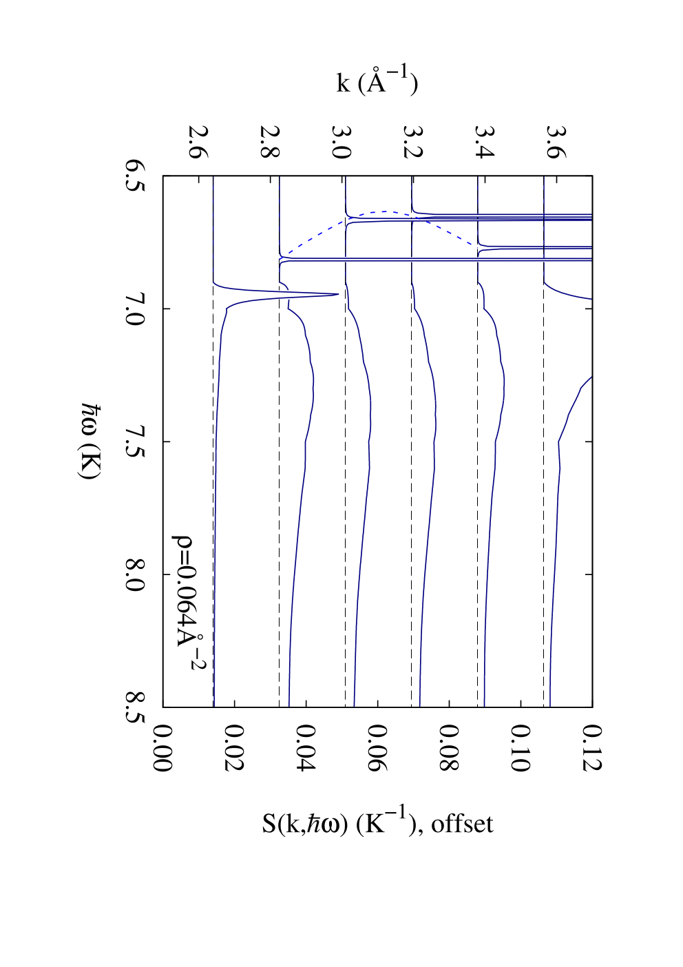
A second striking feature is the appearance of a sharp mode below the plateau. We stress the difference: normally, the plateau is a threshold above which a wave of energy/momentum can decay into two rotons. This has the consequence that the imaginary part of the self-energy is a step function and the real part has a logarithmic singularity [43]. A collective mode is, on the other hand, characterized by a singularity of the . Figs. 2 show, for the two highest densities, the appearance of a sharp discrete mode below the plateau. A close-up of the situation is shown in Fig. 6: Clearly the plateau starts at the same energy for all momenta. At a wave number of Å-1, the collective mode is still merged into the continuum. With increasing wave number, we see, however, a clearly distinguishable mode about 0.3 K below the plateau.
V Discussion
We have already made the essential points of our findings in the discussion of our results. Evidently, the difference between two and three dimensions has quite visible effects on , as mentioned above.
Our findings about a secondary roton should shed some light on the discussion of the nature of the roton minimum. It has been argued [44] that the roton is the “ghost of a vanished vortex ring” or [45, 46] “ghost of a Bragg Spot” due to the imminent liquid-solid phase transition. In this density region two-dimensional 4He already shows a strong signature of the triangular lattice into which it eventually freezes [47, 48, 49] and can exhibit a so called hexatic phase [50].
If the Bragg spot interpretation of the roton is correct, one should perhaps expect a second one and the ratio of the absolute values of the corresponding wave vectors should roughly satisfy because of the triangular lattice of the solid phase.
Our results may indeed be interpreted as an indication that this is the case. It is certainly worth investigating this issue further along the line of angular-dependent excitations [51]. A similar effect has been seen in cold dipolar gases [52] and the relationship is worth examining.
Finally a word about the comparison with simulation data [41]. Overall, the agreement appears satisfactory, most of our results are within the error bars of that calculation. The most visible discrepancy is seen at the highest density of Å-2. At this density, the maxon energy is below twice the roton energy and the modes in this region can decay. One would expect more strength at the decay threshold of as shown by our results whereas the Monte Carlo data indicate – despite large error bars – that the decay strength lies at higher energies. This point deserves further investigation, it might also explain why the maxon energies at Å-2 differ more than expected. Otherwise the agreement is quite good, evidently the strength shown at and above Å-1 follows indeed the kinetic energy branch in both calculations, whereas the plateau region has relatively little strength.
Appendix A Long-wavelength dispersion in 2D
In this appendix, we study the analytic structure of the self-energy as a function of an external energy in the limit . We assume that the solution of the implicit equation (16) has a negligible imaginary part.
We look for processes where a state of wave vector decays into two phonons of wave vectors and . In general one expects, for long wavelengths, a phonon dispersion relation of the form
| (20) |
where is the speed of sound. In fact, it is easily shown that Eq. (16) leads to such a dispersion relation.
The calculation is best carried out in relative and center of mass momenta, i.e. we set
Then, it is clear that
| (21) |
has, for all angles , a relative extremum at . Expanding the energy denominator as
| (22) |
we see that the the value is, at , a relative minimum if (anomalous dispersion) and relative maximum for (normal dispersion). For further reference, abbreviate
We do the calculation first for the case of anomalous dispersion. The three-body coupling matrix element assumes a finite value as , we therefore need to include only the leading term
Then
| (23) | |||||
| (24) |
where and are the values of the energy denominator at and . The integral is imaginary if the denoninator changes its sign for . Since per assumption we have always , therefore we need to have an imaginary part. Then, because of , the imaginary part is picked up for , where
| (25) |
and, hence
| (26) | |||||
For , there is no upper limit of the integration range of the internal momentum, but the integral converges because the three-phonon matrix element goes to zero for large momentum transfers, and the actual value depends on the details of the interaction. However, we are interested only in the non-analytic behavior for . To calculate this behavior, subtract and add the matrix element at the position where the denominator has a second order node, i.e. we write
| (27) |
still contributes to the imaginary part, but not to the non-analytic behavior. We must now distinguish between and . For the former case we have
The momentum integral does not converge, but this is artificial because we have factored out the interaction since we are only interested in the behavior due to the square-root singularity at . Therefore, write for
| (28) | |||||
We can ignore the term because, by assumption, . The integral is then just a numerical value.
For we get
| (29) | |||||
Here, the term dominates in the denominator. Since, by assumption, , the imaginary part has a discontinuity of the order of at .
Appendix B Three-Body Vertex
Normally, the three-body vertex (15) is calculated in convolution approximation. An improvement can be achieved by summing a set of three-body diagrams contributing to , which corresponds topologically to the hypernetted chain (HNC) summation. The first few diagrams are shown in Fig 7.

The equations to be solved are best written in momentum space and relative and center of mass momenta, i.e.
| (30) |
The integral equation to be solved is
| (31) |
where is the set of nodal diagrams, and
is the convolution approximation for this quantity. Also, we have abbreviated
| (32) |
The equations can be easily solved by expanding all functions in terms of , , and the angle between the two vectors, e.g.
This gives us the three-body vertex in the form
Acknowledgements.
We would like to thank C. E. Campbell, F. Gasparini and H. Godfrin for useful discussions. This work was supported, in part, by the Austrian Science Fund FWF under project I602. Additional support was provided by a grant from the Qatar National Research Fund # NPRP NPRP 5 - 674 - 1 - 114.References
- [1] B. Lambert, D. Salin, J. Joffrin, R. Scherm, Journal de Physique Lettres 38(18), 377 (1977)
- [2] W. Thomlinson, J.A. Tarvin, L. Passell, Phys. Rev. Lett. 123, 241 (1980)
- [3] H.J. Lauter, H. Godfrin, V.L.P. Frank, P. Leiderer, in Excitations in Two-Dimensional and Three-Dimensional Quantum Fluids, NATO Advanced Study Institute, Series B: Physics, vol. 257, ed. by A.F.G. Wyatt, H.J. Lauter (Plenum, New York, 1991), NATO Advanced Study Institute, Series B: Physics, vol. 257, pp. 419–427
- [4] H.J. Lauter, H. Godfrin, P. Leiderer, J. Low Temp. Phys. 87, 425 (1992)
- [5] C.C. Chang, M. Cohen, Phys. Rev. B 11, 1059 (1975)
- [6] E. Krotscheck, G.X. Qian, W. Kohn, Phys. Rev. B 31, 4245 (1985)
- [7] E. Krotscheck, Phys. Rev. B 31, 4258 (1985)
- [8] C. Ji, M. Wortis, Phys. Rev. B 34, 7704 (1986)
- [9] J.L. Epstein, E. Krotscheck, Phys. Rev. B 37, 1666 (1988)
- [10] E. Krotscheck, C.J. Tymczak, Phys. Rev. B 45, 217 (1992)
- [11] K.A. Gernoth, J.W. Clark, J. Low Temp. Phys. 96, 153 (1994)
- [12] B.E. Clements, E. Krotscheck, C.J. Tymczak, Phys. Rev. B 53, 12253 (1996)
- [13] R.P. Feynman, Phys. Rev. 94(2), 262 (1954)
- [14] V. Apaja, E. Krotscheck, Phys. Rev. B 64, 134503 (2001)
- [15] H.W. Jackson, E. Feenberg, Ann. Phys. (NY) 15, 266 (1961)
- [16] H.W. Jackson, E. Feenberg, Rev. Mod. Phys. 34(4), 686 (1962)
- [17] C.C. Chang, C.E. Campbell, Phys. Rev. B 13(9), 3779 (1976)
- [18] B.E. Clements, H. Godfrin, E. Krotscheck, H.J. Lauter, P. Leiderer, V. Passiouk, C.J. Tymczak, Phys. Rev. B 53, 12242 (1996)
- [19] C.E. Campbell, E. Krotscheck, T. Lichtenegger, in preparation (2014)
- [20] C.E. Campbell, B. Fåk, H. Godfrin, E. Krotscheck, H.J. Lauter, T. Lichtenegger, J. Ollivier, H. Schober, A. Sultan, in preparation (2014)
- [21] H.M. Böhm, R. Holler, E. Krotscheck, M. Panholzer, Phys. Rev. B 82(22), 224505/1 (2010)
- [22] E. Krotscheck, T. Lichtenegger, in preparation (2014)
- [23] C.E. Campbell, E. Krotscheck, J. Low Temp. Phys. 158, 226 (2010)
- [24] H. Godfrin, M. Meschke, H.J. Lauter, A. Sultan, H.M. Böhm, E. Krotscheck, M. Panholzer, Nature 483, 576–579 (2012)
- [25] E. Vitali, M. Rossi, L. Reatto, D.E. Galli, Phys. Rev. B 82, 174510 (2010)
- [26] A. Roggero, F. Pederiva, G. Orlandini, Phys. Rev. B 88, 094302 (2013)
- [27] M. Nava, D.E. Galli, S. Moroni, E. Vitali, Phys. Rev. B 87, 145506 (2013)
- [28] E. Feenberg, Theory of Quantum Fluids (Academic, New York, 1969)
- [29] R.A. Aziz, V.P.S. Nain, J.C. Carley, W.J. Taylor, G.T. McConville, J. Chem. Phys. 70, 4330 (1979)
- [30] J. Boronat, in Microscopic Approaches to Quantum Liquids in Confined Geometries, ed. by E. Krotscheck, J. Navarro (World Scientific, Singapore, 2002), pp. 21–90
- [31] C.C. Chang, C.E. Campbell, Phys. Rev. B 15(9), 4238 (1977)
- [32] E. Krotscheck, Phys. Rev. B 33, 3158 (1986)
- [33] P. Kramer, M. Saraceno, Geometry of the time-dependent variational principle in quantum mechanics, Lecture Notes in Physics, vol. 140 (Springer, Berlin, Heidelberg, and New York, 1981)
- [34] A.K. Kerman, S.E. Koonin, Ann. Phys. (NY) 100, 332 (1976)
- [35] R.P. Feynman, M. Cohen, Phys. Rev. 102, 1189 (1956)
- [36] H.W. Jackson, Phys. Rev. A 8, 1529 (1973)
- [37] D.K. Lee, F.J. Lee, Phys. Rev. B 11, 4318 (1975)
- [38] C.E. Campbell, Phys. Lett. A 44, 471 (1973)
- [39] C.E. Campbell, E. Krotscheck, Phys. Rev. B 80, 174501/1 (2009)
- [40] M. Saarela, V. Apaja, J. Halinen, in Microscopic Approaches to Quantum Liquids in Confined Geometries, ed. by E. Krotscheck, J. Navarro (World Scientific, Singapore, 2002), pp. 139–205
- [41] F. Arrigoni, E. Vitali, D.E. Galli, L. Reatto. Excitation spectrum in two-dimensional superfluid 4He (2013). ArXiv:cond-mat/1305.3732
- [42] V. Apaja, J. Halinen, V. Halonen, E. Krotscheck, M. Saarela, Phys. Rev. B 55, 12925 (1997)
- [43] L.P. Pitaevskii, Zh. Eksp. Theor. Fiz. 36, 1168 (1959). [Sov. Phys. JETP 9, 830 (1959)]
- [44] R.P. Feynman, Progress in Low Temperature Physics (North Holland, Amsterdam, 1955), vol. I, chap. 2
- [45] P. Nozières, J. Low Temp. Phys. 137, 45 (2004)
- [46] P. Nozières, J. Low Temp. Phys. 142(1-2), 91 (2006)
- [47] P. Whitlock, G. Chester, M. Kalos, Phys. Rev. B 38(4), 2418 (1988)
- [48] J. Halinen, V. Apaja, K. Gernoth, M. Saarela, J. Low Temp. Phys. 121(5-6), 531 (2000)
- [49] V. Apaja, J. Halinen, M. Saarela, Physica B: Condensed Matter 284, 29 (2000)
- [50] V. Apaja, M. Saarela, EPL (Europhysics Letters) 84(4), 40003 (2008)
- [51] A.D. Jackson, B.K. Jennings, R.A. Smith, A. Lande, Phys. Rev. B 24, 105 (1981)
- [52] A. Macia, D. Hufnagl, F. Mazzanti, J. Boronat, R.E. Zillich, Phys. Rev. Lett. 109, 235307 (2012)