Halo Mass Dependence of H i and O vi Absorption: Evidence for Differential Kinematics

We have assembled a sample of 14 galaxies in the fields of UV bright quasars with high resolution HST imaging and ultraviolet spectra. We impose four primary criteria for the galaxy sample: (1) each galaxy must be intervening to a background quasar within a projected distance of 300 kpc from the line of sight and must have a spectroscopic redshift measurement, (2) each galaxy must be imaged with the Hubble Space Telescope (HST), (3) a HST/COS and/or STIS spectrum of the background quasar is available that, at a minimum, covers the redshifted Ly $\alpha$, Ly $\beta$, and O vi $\lambda\lambda 1031,1037$ transitions within $\pm 1000$ km s^-1 of the associated foreground galaxy redshift, and (4) the foreground galaxy must not reside in a group or cluster environment to the extent that the data provides such information.

The 300 kpc projected distance allows us to study the CGM out to the extent probed by Steidel et al. [68], Prochaska et al. [58], and Rudie et al. [60] and to extend beyond the 150 kpc range probed by Tumlinson et al. [83], Tumlinson et al. [84]. The HST/WFPC2 images provide the spatial information required to measure galaxy morphological parameters and determine galaxy orientations relative to the quasar line of sight. The HST/COS and/or STIS spectroscopy allows Voigt profile decomposition of the Ly $\alpha$, Ly $\beta$, and O vi $\lambda\lambda 1031,1037$ absorption profiles, providing individual “cloud” column densities and kinematics.

By selecting isolated field galaxies, we aim to study the CGM independent of galaxy environment. In a given quasar field, we first require that no other galaxy is identified within $\pm 1000~{\hbox{km~s${}^{-1}$}}$ (based upon redshift). If other galaxies exist in the field within this velocity window, we then require the galaxies lie farther than a projected distance of $600~\mathrm{kpc}$ from the quasar line of sight.

The quasar fields from which the galaxy sample is drawn were surveyed by Ellingson & Yee [26], Lanzetta et al. [41], Le Brun et al. [42], Chen et al. [13], and Johnson et al. [33]. We note that the fields have been studied for different science goals employing different facilities to varying degrees of completeness. A detailed discussion of the application of the galaxy selection criteria for each field is presented in Appendix A. Here, we briefly summarize the surveys. The galaxies observed by Ellingson & Yee [26] have redshifts $0.3<z<0.6$ and are intervening to radio-selected quasars. The galaxies surveyed by Lanzetta et al. [41], Le Brun et al. [42], and Chen et al. [13] have redshifts $0.05<z<0.8$ are selected on the basis that HST/FOS spectra of the quasar had been obtained for the HST Key Project [1, cf.,].

The resulting redshift range of our galaxy sample is determined exclusively by the UV spectral coverage of the HST/COS and STIS observations and not by any a priori redshift cuts. Using the above four selection criteria, we compiled a sample of 14 galaxies spanning the redshift range of $0.12\leq z\leq 0.67$ with impact parameters from $60\leq D\leq 290$ kpc.

In Table 1, we list the observational data employed for the sample galaxies. Column (1) lists the quasar field [B1950 designation]. Column (2) lists the imaging and spectroscopic instruments. Column (3) lists the imaging filter and the COS or STIS grating. Columns (4) and (5) list the exposure time and the program ID, respectively.

All HST/WFPC2 images were obtained using the F702W band. We adopted the reduced and calibrated images from the WFPC-2 Associations Science Products Pipeline (WASPP¹¹ 1 http://archive.stsci.edu/hst/wfpc2/pipeline.html).

The galaxy apparent Vega magnitudes, $m_{\hbox{\tiny F702W}}$, were determined using $1.5~\sigma$ isophotes from Source Extractor [4]. From the galaxy centroids, we compute the galaxy offset from the quasar (arcsec) and the galaxy-quasar sightline impact parameter (kpc). We computed AB $r$-band absolute magnitudes, $M_{r}$, by $k$-correcting the observed F702W magnitudes following the method of Nielsen et al. [52]. To determine galaxy virial masses, $M_{\rm\,h}$, we performed halo abundance matching [2, 81, e.g.,] following the method of Churchill et al. [18], in which we match the distribution of the maximum circular velocity of halos in the Bolshoi $N$-body cosmological simulation of Klypin et al. [40] to the COMBO-17 $r$-band luminosity function of Wolf et al. [88]. Galaxy virial radii are then computed from $M_{\rm\,h}$ using the relation of Bryan & Norman [9]. Uncertainties in the viral masses and virial radii, which are on the order 10%, originate from the scatter in the virial mass circular velocity distribution function [see 18, for details].

Quantified galaxy morphological parameters were measured using GIM2D [67] following the methods of Kacprzak et al. [35]. GIM2D models the two-dimensional brightness profiles of the galaxies and computes the inclination, $i$, and the position angle, $\Phi$, on the sky. We adopt the formalism that $i=0^{\circ}$ is face-on and $i=90^{\circ}$ is edge-on. We translate the position angle to an “azimuthal angle” defined such that for $\Phi=0^{\circ}$ the quasar sightline lies along the projected major axis, and for $\Phi=90^{\circ}$ it lies along the galaxy projected minor axis.

In Table 2, columns (1) and (2) list the quasar field and the galaxy spectroscopic redshift. Columns (3)–(5) list the galaxy offsets relative to the quasar and the galaxy impact parameter, respectively. Columns (6) and (7) list the galaxy HST/WFPC2 F702W apparent magnitude (Vega) and the $r$-band absolute magnitude (AB). Columns (8) and (9) list the virial mass and virial radius of the galaxy. Columns (10) and (11) list the galaxy azimuthal angle and inclination.

The galaxy WFPC/F702W apparent magnitudes range from $22.6\geq m_{\hbox{\tiny F702W}}\geq 17.8$. Absolute $r$-band magnitudes range from $-15.5\geq M_{r}\geq-20.2$. The range of galaxy inclinations and azimuthal angles are $18^{\circ}\leq i\leq 85^{\circ}$ and $6^{\circ}\leq\Phi\leq 87^{\circ}$, respectively. The virial masses range from $10.8\leq\log(M_{\rm\,h}/M_{\odot})\leq 12.2$, with virial radii between $70\leq R_{\rm vir}\leq 225~\mathrm{kpc}$. The median virial mass is $\log(M_{\rm\,h}/M_{\odot})=11.5$.

The HST/COS spectra were reduced and flux calibrated using the CalCOS pipeline (V2.11). Vacuum and heliocentric corrections, dispersion alignment, and co-addition of individual exposures were performed using software developed by the COS team²² 2 http://casa.colorado.edu/$\!\sim\!$danforth/science/cos/costools.html [49, also see].

Reduction and calibration of the E140M HST/STIS spectrum (for Q1704$+$6048 using the $0.2^{\prime\prime}\times 0.2^{\prime\prime}$ slit) was performed using the standard STIS pipeline [8]. Further details are discussed in Narayanan et al. [48]. Continuum fitting for both the HST/COS and HST/STIS data sets was conducted using the interactive SFIT task in IRAF³³ 3 IRAF is distributed by the National Optical t Astronomy Observatory, which is operated by the Association of Universities for Research in Astronomy (AURA) under cooperative agreement with the National Science Foundation. following the methods described in Sembach & Savage [65]. We then refined higher order continuum fits using our own code, Fitter [15].

We searched the quasar spectra for Ly $\alpha$, Ly $\beta$, and O vi $\lambda\lambda 1031,1037$ absorption within $\pm 1000$ km s^-1 of the identified galaxy redshift. We adopt the objective detection methods of [64] using the $5~\sigma$ uncertainty in the equivalent width spectrum. Once an absorption feature is identified, we use the methods of Churchill et al. [17] and Churchill & Vogt [19] to measure the velocity extremes of the absorption, $v^{\,(-)}$ and $v^{\,(+)}$, the rest-frame equivalent widths, $W_{r}$, and the optical depth mean system absorption redshifts, $z_{\rm abs}$, using the Ly $\alpha$ absorption feature.

For an absorption feature to be adopted as a detection, we apply the criterion of a $3~\sigma$ equivalent width significance level, i.e., $W_{r}\geq 3\sigma_{W_{r}}$, otherwise we quote $3\sigma_{W_{r}}$ as the upper limit on $W_{r}$. The quoted uncertainties in the measured equivalent widths account for both the pixel statistical uncertainty and the systematic uncertainty due to the choice of continuum fit. The latter assumes a mean continuum placement uncertainty of 30% of the mean pixel statistical uncertainty [65, see]. Depending on the signal-to-noise ratio of the spectral region, the continuum uncertainty yields a 5–20 mÅ systematic uncertainty in the equivalent width.

To verify the identity of Ly $\alpha$ absorption, we examine whether the associated Ly $\beta$ absorption is formally detected. Further verification is obtained by detection of the O vi doublet; however, not all Ly $\alpha$ absorption has detected Ly $\beta$ and/or metal-line absorption. In the case of the O vi doublet, we do not require that both members of the doublet are formally detected in order to identify either O vi $\lambda 1031$ or O vi $\lambda 1037$ absorption (either due to line blending or the $\lambda 1037$ absorption being below the required significance level). The Ly $\alpha$ transition was detected for all but one of the galaxy-absorber pairs. For all but four galaxy-absorber pairs, Ly $\beta$ was detected, but O vi was detected for three of these four pairs. For only one pair, no Ly $\alpha$, Ly $\beta$, nor O vi was detected.

To quantify the absorption column densities and kinematics, we fitted the absorption line using Voigt profile (VP) decomposition. Each VP component is described by three physical parameters, the column density, Doppler $b$ parameter, and the velocity center. We employed the code Minfit [19], adopting the philosophy of enforcing the minimum number of statistically required VP components to model an absorption system (i.e., simultaneously to all transitions). Details of the fitting procedure are described in [27]. We tie the velocity centers for each VP component across all ions. We also assume the line broadening is dominated by a Gaussian turbulent component; therefore, each VP component at a given velocity has the same Doppler $b$ parameter. The latter assumption is motivated by the simulations of Oppenheimer & Davé [54] in which sub-resolution turbulence was required for modeling O vi absorbing gas in order to reproduce the observed column density and $b$ parameter distributions. The one exception is $z_{\rm gal}=0.1963$ absorption in the spectrum of Q1259$+$5920, where a satisfactory VP model required thermal scaling of the Doppler $b$ parameters.

Though Ly $\gamma$ is detected for several, but not all of the absorption systems, we quote VP model results only from simultaneous fits to the Ly $\alpha$ and Ly $\beta$ transitions (except in three systems in which only Ly $\alpha$ was detected). Muzahid [47] showed that Ly $\alpha$ and Ly $\beta$ absorption primarily traces the high ionization phase where O vi arises, whereas the higher order Lyman series line profiles are dominated by the lower ionization phase giving rise to C ii, Si ii, C iii, and Si iii absorption. Thus, by omitting higher order Lyman series lines we do not lose information on the O vi phase. Most importantly, by omitting higher order H i Lyman series lines, even when they are detected, we present a uniform analysis of the absorption systems. In Appendix B, we compare the derived H i column densities, $N({\hbox{{\rm H}\kern 1.00006pt{\sc i}}})$, obtained from Ly $\alpha$+Ly $\beta$ VP models and Ly $\alpha$+Ly $\beta$+Ly $\gamma$ VP models for systems for which Ly $\gamma$ is also detected. The exercise demonstrates that the inclusion of Ly $\gamma$ does not discernibly alter our derived $N({\hbox{{\rm H}\kern 1.00006pt{\sc i}}})$ values.

In the case of line blending (overlapping absorption from transitions associated with systems at other redshifts), when possible, we carefully decompose the lines using the procedure illustrated in Appendix C. The deblending technique is designed to recover the shape of the profile for the target transition.

Results of the absorption line analysis are listed in Table 3. Column (1) gives the quasar field. Columns (2) and (3) list the spectroscopic galaxy redshift and the absorption redshift. Columns (4)–(6) list the measured rest-frame equivalent widths of the Ly $\alpha$, Ly $\beta$, and O vi $\lambda 1031$ absorption profiles. Columns (7) and (8) give the system total H i and O vi column densities, which are the sums of the VP components in each system. Columns (9) and (10) list the maximum blueward and redward velocity limits of the Ly $\alpha$ absorption profiles.

The range of rest-frame equivalent widths is $0.05\leq W_{r}(\hbox{{\rm Ly}\kern 1.00006pt$\alpha$})\leq 1.54$ Å and $0.02\leq W_{r}(1031)\leq 0.45$ Å, corresponding to the system total column densities ranges $13.1\leq\log N({\hbox{{\rm H}\kern 1.00006pt{\sc i}}})\leq 18.5$ and $13.4\leq\log N({\hbox{{\rm O}\kern 1.00006pt{\sc vi}}})\leq 14.7$, respectively. The maximum blueward and redward velocities of the Ly $\alpha$ absorption are $v^{\,(-)}=-1020$ km s^-1 and $v^{\,(+)}=440$ km s^-1, respectively.

In Figure 1, we show three of the 14 galaxy-absorber pairs in our sample. The remaining 11 galaxies and their associated absorption are presented in Appendix A.

For each galaxy-absorber pair, we present a portion of the HST/WFPC2 image centered on the galaxy and the Ly $\alpha$, Ly $\beta$, and O vi $\lambda\lambda 1031,1037$ absorption profiles. In the galaxy image, the arrow points in the direction of the quasar line of sight. A bar provides that scale of 10 kpc in the galaxy rest frame. The legend provides the galaxy impact parameter, $D$, inclination, $i$, and azimuthal angle, $\Phi$. The Voigt profile models of the absorption lines are the red curves superimposed on the black data. The velocity centroid of each VP component is shown by the red ticks above the continuum normalized spectra. The velocity zero-point of each spectrum is taken to be galaxy systemic velocity.

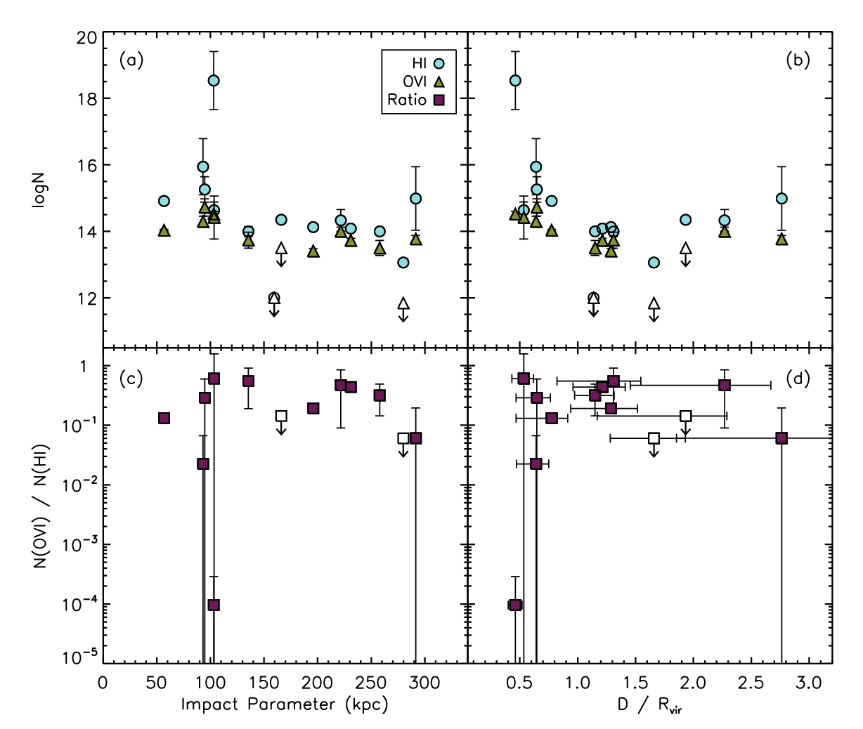
In Figure 2, we present the spatial behavior of the system total H i column density, $N({\hbox{{\rm H}\kern 1.00006pt{\sc i}}})$, and the system total O vi column density, $N({\hbox{{\rm O}\kern 1.00006pt{\sc vi}}})$. The system total column densities are the sums of the individual Voigt profile component column densities. We color the $N({\hbox{{\rm H}\kern 1.00006pt{\sc i}}})$ points sky-blue, the $N({\hbox{{\rm O}\kern 1.00006pt{\sc vi}}})$ points green, and the ratio $N({\hbox{{\rm O}\kern 1.00006pt{\sc vi}}})/N({\hbox{{\rm H}\kern 1.00006pt{\sc i}}})$ magenta. Upper limits are shown as open circles with downward arrows.

In Figure 2(a), we plot $N({\hbox{{\rm H}\kern 1.00006pt{\sc i}}})$ and $N({\hbox{{\rm O}\kern 1.00006pt{\sc vi}}})$ versus impact parameter, $D$. The total $N({\hbox{{\rm H}\kern 1.00006pt{\sc i}}})$ is typically $\log N({\hbox{{\rm H}\kern 1.00006pt{\sc i}}})=14$ out to $D\sim 300$ kpc (we note that one system has a stringent upper limit of $\log N({\hbox{{\rm H}\kern 1.00006pt{\sc i}}})<12$). Though higher $N({\hbox{{\rm H}\kern 1.00006pt{\sc i}}})$ systems are found at $D<100$ kpc, there is no statistical trend between $N({\hbox{{\rm H}\kern 1.00006pt{\sc i}}})$ and $D$. A Kendall-$\tau$ rank correlation test, which includes upper limits, yields a $1.8~\sigma$ consistency with the null hypothesis of no correlation.

We find $N({\hbox{{\rm O}\kern 1.00006pt{\sc vi}}})$ out to $\sim\!290$ kpc to a limit of $\log N({\hbox{{\rm O}\kern 1.00006pt{\sc vi}}})=12.8$. We note that the detection at $D=292$ kpc (in Q0454$-$132 at $z=0.4100$) is very tentative (see Figure 1). If that detection were deemed an upper limit, then our data show O vi absorption out to $\sim\!260$ kpc. Similar to the behavior with $N({\hbox{{\rm H}\kern 1.00006pt{\sc i}}})$, we find no statistically significant trend between $N({\hbox{{\rm O}\kern 1.00006pt{\sc vi}}})$ and $D$ (only a $2.5~\sigma$ trend).

In Figure 2(b), we plot $N({\hbox{{\rm H}\kern 1.00006pt{\sc i}}})$ and $N({\hbox{{\rm O}\kern 1.00006pt{\sc vi}}})$ versus $D/R_{\rm vir}$. There is a higher average value and a broader spread in $N({\hbox{{\rm H}\kern 1.00006pt{\sc i}}})$ for $D/R_{\rm vir}<1$ as compared to $D/R_{\rm vir}>1$, with $\log\langle N({\hbox{{\rm H}\kern 1.00006pt{\sc i}}})\rangle=15.9\pm 1.6$ inside the projected virial radius and $\log\langle N({\hbox{{\rm H}\kern 1.00006pt{\sc i}}})\rangle=14.1\pm 0.5$. outside the projected virial radius. In We find that the $N({\hbox{{\rm O}\kern 1.00006pt{\sc vi}}})$ values inside and outside of the projected virial radius lie within one standard deviation of the average $\log\langle N({\hbox{{\rm O}\kern 1.00006pt{\sc vi}}})\rangle=14.03\pm 0.44$. We do not see a larger dispersion in $N({\hbox{{\rm O}\kern 1.00006pt{\sc vi}}})$ at $D/R_{\rm vir}<1$ as seen for H i.

The ratio $N({\hbox{{\rm O}\kern 1.00006pt{\sc vi}}})/N({\hbox{{\rm H}\kern 1.00006pt{\sc i}}})$ is shown in Figures 2(c) and 2(d) as a function of $D$ and $D/R_{\rm vir}$, respectively. Due to the flat spatial distribution of $N({\hbox{{\rm O}\kern 1.00006pt{\sc vi}}})$ and the higher dispersion of $N({\hbox{{\rm H}\kern 1.00006pt{\sc i}}})$ at $D/R_{\rm vir}<1$, the spread in $N({\hbox{{\rm O}\kern 1.00006pt{\sc vi}}})/N({\hbox{{\rm H}\kern 1.00006pt{\sc i}}})$ is a factor of $\simeq 8$ greater inside than outside the projected virial radius, with $\sigma(D/R_{\rm vir}\!\leq\!1)=1.5$ and $\sigma(D/R_{\rm vir}\!>\!1)=0.18$.

The different spreads in the $N({\hbox{{\rm O}\kern 1.00006pt{\sc vi}}})/N({\hbox{{\rm H}\kern 1.00006pt{\sc i}}})$ inside and outside the projected virial radius are driven by the spatial behavior of H i. Inside the projected virial radius, $N({\hbox{{\rm H}\kern 1.00006pt{\sc i}}})$ has a larger dispersion than outside this region, whereas $N({\hbox{{\rm O}\kern 1.00006pt{\sc vi}}})$ has a small dispersion both inside and outside the projected virial radius. The O vi column densities inside the projected virial radius appear to be similar to those outside this region, whereas the quantity of H i can be variable.

To ensure we have a fair sample with which we can examine the geometric distribution of H i and O vi absorption around the galaxies, we performed Kolmogorov-Smirnov (KS) tests to determine whether the observed distributions of galaxy azimuthal angles, $\Phi$, and inclinations, $i$, are consistent with being drawn from the distributions expected for an unbiased sample. For $\Phi$, the KS test probability is $P({\rm KS})=0.62$ and for $i$ the probability is $P({\rm KS})=0.46$. We conclude that both $\Phi$ and $i$ are consistent with unbiased distributions.

In Figure 3(a) and 3(b), we show the system total $N({\hbox{{\rm H}\kern 1.00006pt{\sc i}}})$, $N({\hbox{{\rm O}\kern 1.00006pt{\sc vi}}})$, and $N({\hbox{{\rm O}\kern 1.00006pt{\sc vi}}})/N({\hbox{{\rm H}\kern 1.00006pt{\sc i}}})$, respectively, versus inclination. The uncertainties in the inclination measurements derived from GIM2D are shown only in Figure 3(b). A Kendall-$\tau$ test (including limits) yields no trend in the $N({\hbox{{\rm H}\kern 1.00006pt{\sc i}}})$ distribution ($1.1~\sigma$), the $N({\hbox{{\rm O}\kern 1.00006pt{\sc vi}}})$ distribution ($0.8~\sigma$), nor in the distribution of the ratio $N({\hbox{{\rm O}\kern 1.00006pt{\sc vi}}})/N({\hbox{{\rm H}\kern 1.00006pt{\sc i}}})$ ($0.8~\sigma$) with galaxy inclination. Whether a galaxy is observed with a face-on or an edge-on orientation, there appears to be a relatively flat distribution of H i and O vi column densities.

In Figure 4(a) and 4(b), we present the system total $N({\hbox{{\rm H}\kern 1.00006pt{\sc i}}})$, $N({\hbox{{\rm O}\kern 1.00006pt{\sc vi}}})$, and $N({\hbox{{\rm O}\kern 1.00006pt{\sc vi}}})/N({\hbox{{\rm H}\kern 1.00006pt{\sc i}}})$, respectively, versus azimuthal angle, $\Phi$. The uncertainties in the azimuthal angle measurements derived from GIM2D are shown only in Figure 4(b) but apply for all panels. A Kendall-$\tau$ test (including limits) yields no statistical signature for a correlation between H i column density and $\Phi$ ($0.4~\sigma$). We do note that the $N({\hbox{{\rm H}\kern 1.00006pt{\sc i}}})$ values appear to increase toward the projected major axis ($\Phi=0^{\circ}$) and the projected minor axis ($\Phi=90^{\circ}$).

To crudely estimate the degree to which the two largest $N({\hbox{{\rm H}\kern 1.00006pt{\sc i}}})$ absorbers (which are most closely aligned with the projected axes) may be outliers of the distribution of H i absorbers, we calculated the mean and standard deviation of the $N({\hbox{{\rm H}\kern 1.00006pt{\sc i}}})$ excluding the two largest $N({\hbox{{\rm H}\kern 1.00006pt{\sc i}}})$ absorbers. We obtained $\log\langle N({\hbox{{\rm H}\kern 1.00006pt{\sc i}}})\rangle=14.47\pm 0.74$. The two largest $N({\hbox{{\rm H}\kern 1.00006pt{\sc i}}})$ absorbers lie at $2.8~\sigma$ and $5.5~\sigma$ from $\langle N({\hbox{{\rm H}\kern 1.00006pt{\sc i}}})\rangle$. For this small sample, the $N({\hbox{{\rm H}\kern 1.00006pt{\sc i}}})$ of the system most closely aligned with the projected minor axis is an outlier of the $N({\hbox{{\rm H}\kern 1.00006pt{\sc i}}})$ distribution in that it has a significantly larger column density. A statistical signature for an H i column density enhancement toward the projected major axis is less convincing.

We further examine the apparent trend for increasing $N({\hbox{{\rm H}\kern 1.00006pt{\sc i}}})$ toward the projected major and minor axes by symmetrically folding the azimuthal angle about $45^{\circ}$, such that $0^{\circ}$ corresponds to alignment along either the major or the minor projected axis and $45^{\circ}$ corresponds to a $45^{\circ}$ azimuthal angle with respect to either axis. A Kendall-$\tau$ test (including limits) on the folded distribution yields no statistical signature for an anti-correlation between $N({\hbox{{\rm H}\kern 1.00006pt{\sc i}}})$ and angular separation away from the galaxy projected axes ($1.7~\sigma$). If a trend exists, our sample is too small to reveal a statistical significance.

In the case of O vi, the azimuthal distribution of $N({\hbox{{\rm O}\kern 1.00006pt{\sc vi}}})$ appears uniform, or flat, for all galaxy orientations. Computing the mean and standard deviation (omitting limits), we obtain $\log\langle N({\hbox{{\rm O}\kern 1.00006pt{\sc vi}}})\rangle=14.05\pm 0.42$ and find no outlying measurements with detected O vi absorption.

For the ratio $N({\hbox{{\rm O}\kern 1.00006pt{\sc vi}}})/N({\hbox{{\rm H}\kern 1.00006pt{\sc i}}})$, the two absorbers within $\pm 10^{\circ}$ of the major and minor axes show a smaller ratio compared to the data in the range $10^{\circ}\leq\Phi\leq 80^{\circ}$. Excluding these two absorbers and the two absorbers with upper limits, the mean and standard deviation is $\log\langle N({\hbox{{\rm O}\kern 1.00006pt{\sc vi}}})/N({\hbox{{\rm H}\kern 1.00006pt{\sc i}}})\rangle=-0.61\pm 0.45$. Compared to this distribution, the $\Phi\simeq 6^{\circ}$ absorber is a $\sim\!4~\sigma$ outlier and the $\Phi\simeq 87^{\circ}$ absorber is a $\sim\!8~\sigma$ outlier. Since the $N({\hbox{{\rm O}\kern 1.00006pt{\sc vi}}})$ distribution is flat with azimuthal angle, whereas the $N({\hbox{{\rm H}\kern 1.00006pt{\sc i}}})$ distribution exhibits higher values near the projected axes, the smaller $N({\hbox{{\rm O}\kern 1.00006pt{\sc vi}}})/N({\hbox{{\rm H}\kern 1.00006pt{\sc i}}})$ ratios in these two absorbers are driven by their higher $N({\hbox{{\rm H}\kern 1.00006pt{\sc i}}})$. We infer that the chemical and/or ionization conditions of the hot CGM are globally distributed, if patchy, for all azimuthal angles more than $\pm 10^{\circ}$ away from the projected major and minor axes (acknowledging some variation as suggested by the few upper limits).

For visualization purposes, in Figure 5(a) and Figure 5(b), we illustrate the relationship between the two-dimensional projected location of the absorbing gas and the system total $N({\hbox{{\rm H}\kern 1.00006pt{\sc i}}})$ and $N({\hbox{{\rm O}\kern 1.00006pt{\sc vi}}})$, respectively. The projected geometric position of the quasar sightlines are computed with respect to the virial radius using the relations $D/R_{\rm vir}\cos(\Phi)$ for projection along the galaxy major axis, and $D/R_{\rm vir}\sin(\Phi)$ for projection along the galaxy minor axis. Data point colors correspond to absorber column density according to the color scale on the right. Upper limits are plotted as open circles.

Most galaxies probed at $D/R_{\rm vir}>1$ in this sample have moderate column density absorption with $\log N({\hbox{{\rm H}\kern 1.00006pt{\sc i}}})\simeq 14$ located at intermediate azimuthal angles, between $10^{\circ}$ and $90^{\circ}$. In turn, the galaxies probed at $D/R_{\rm vir}<1$ exhibit high column density absorption along their projected major and minor axes. Though the sample is small and the realization of the data may not be a full representation of a larger sample, our data suggest a picture in which moderate column density H i and O vi gas is distributed around galaxies out to greater than $2R_{\rm vir}$, with higher column density H i aligned near the galaxy projected major and minor axes for $D<R_{\rm vir}$.

The detection threshold sensitivity for absorption is not uniform from absorber to absorber due to varying signal-to-noise ratios, $S/N$, of the quasar spectra. Thus, for example, weak absorption at high relative velocity that could be detected in a high $S/N$ spectral region for one system, might not be detectable for a different system appearing in a lower $S/N$ spectral region. In conducting our kinematic analysis, we first examine the non-uniformity of the detection sensitivity.

In Figure 6, we present the cumulative distribution (CDF) of the $3~\sigma$ equivalent width detection limits for both Ly $\alpha$ and O vi $\lambda 1031$ absorption. The detection thresholds are the $3~\sigma$ equivalent width uncertainties for unresolved lines [64, 15, cf.,] averaged over $\pm 1000$ km s^-1 relative to the galaxy redshift assuming unresolved absorption lines. The sample is 100% complete for absorption features greater than $W_{r}({\hbox{{\rm Ly}\kern 1.00006pt$\alpha$}})=0.062$ Å and $W_{r}(1031)=0.032$ Å, indicating that we generally have higher $S/N$ spectral coverage for O vi absorption. All but two of the individual absorption features in the sample have measured equivalent widths above the 100% completeness level. For our analysis, we removed these two features.

In Figure 7(a), we plot the velocity offset between the Voigt profile component “clouds” with the highest $N({\hbox{{\rm O}\kern 1.00006pt{\sc vi}}})$ and each H i absorbing cloud as a function of $D/R_{\rm vir}$. The dotted line at $v_{\hbox{\tiny OVI}}-v_{\hbox{\tiny HI}}=0$ indicates no velocity offset between the H i clouds and the highest $N({\hbox{{\rm O}\kern 1.00006pt{\sc vi}}})$ cloud. Most H i and O vi absorbing clouds are clustered within $\sim\!500$ km s^-1.

The data also reveal that the highest $N({\hbox{{\rm O}\kern 1.00006pt{\sc vi}}})$ cloud in a system does not align kinematically with the highest $N({\hbox{{\rm H}\kern 1.00006pt{\sc i}}})$ cloud in every case. To further illustrate, we plot the velocity offset between the highest $N({\hbox{{\rm O}\kern 1.00006pt{\sc vi}}})$ cloud and the highest $N({\hbox{{\rm H}\kern 1.00006pt{\sc i}}})$ cloud in a system in Figure 7(b). In 5 of 10 systems with detected O vi absorption, we observe a velocity offset between the bulk of the neutral hydrogen and the bulk of the O vi. In three of these cases, the velocity offset is $\sim\!100$ km s^-1. Since a velocity offset implies spatially separated absorbing clouds, we can infer physically distinct phases of gas (different densities, temperatures, and metallicities) in roughly half of the sightlines through the CGM, as probed using O vi and H i as a tracer of the gas phase. Examining absorption from the low ions such as C ii, Si ii, etc., would be instrumental in examining whether this is the case. Unfortunately, the mean $N({\hbox{{\rm H}\kern 1.00006pt{\sc i}}})$ for our sample is roughly 1.5 dex below the threshold where low ion metals can be detected in spectra with moderate signal-to-noise ratios [32].

In Figure 8, we plot the velocity difference between the individual Voigt profile component “clouds” and the galaxy systemic velocity, $\Delta v=v_{\rm cld}-v_{\rm gal}=c(z_{\rm cld}-z_{\rm gal})/(1+z_{\rm gal})$, as a function of halo mass, $M_{\rm\,h}$. Data point colors denote the $D/R_{\rm vir}$ location of the absorption, where sky-blue corresponds to $D/R_{\rm vir}\leq 1$, green between $1<D/R_{\rm vir}\leq 2$, and $D/R_{\rm vir}>2$ is magenta. For our sample, we find that $\sim\!70$% of H i absorbing components lie within $\pm 200$ km s^-1 of the galaxy systemic velocity, $\sim\!80$% lie within $\pm 300$ km s^-1, and $\sim\!90$% lie within $\pm 500$ km s^-1. For O vi, we find $\sim\!90$%, $\sim\!95$%, and $100$% lie within $\pm 200$, $\pm 300$, and $\pm 500$ km s^-1, respectively.

To investigate whether clouds have relative line of sight velocities that exceed or do not exceed the escape velocity of the halo in which they reside, we computed the escape velocity for each galaxy [68, cf.,],

for each galaxy at $R=R_{\rm vir}$, $2R_{\rm vir}$, and $3R_{\rm vir}$, where $R$ is galactocentric distance, and superimposed the results on Figure 8 as colored lines corresponding to the three values of $R$. A [50] (NFW) dark matter halo profile is assumed with mean concentration parameter, $c\,(M_{\rm h},z_{\rm gal})$, computed from the relation of [10]. The curves are not smooth with increasing virial mass due to the redshift dependence of the concentration parameter.

The galactocentric distances of the clouds are not known, only constrained to lie at $R\geq D$. Assuming cloud galactocentric distances at multiples of the virial radius, and comparing same-colored points and curves, we find $\sim\!40$% of H i cloud components have relative velocities in excess of the galaxy escape velocity. Roughly $60$% of the clouds that reside outside the virial radius (green and magenta data) have velocities exceeding the escape velocity, whereas only $\sim\!15$% of clouds, if they reside at the virial radius (sky-blue data/lines), have greater than escape velocities.

In Figure 9, we show the absolute relative velocity of the absorption with respect to the galaxy normalized to the escape velocity, $\left|\Delta v/v_{\rm esc}\right|$, versus virial mass. We also show the galaxy stellar mass, $M_{\ast}$, based upon the stellar mass to halo mass functions of Moster et al. [46]. Data points are colored by $D/R_{\rm vir}$ using the same designations as in Figure 8. For this exercise, we assume $R=D$ for the absorbing clouds, which provides the upper limit to the escape velocity. Thus, the points plotted in Figure 9 are lower limits on $\left|\Delta v/v_{\rm esc}\right|$. Characteristic error bars are shown on the left-most data points in each panel. Points that lie above the dotted line at $\left|\Delta v/v_{\rm esc}\right|=1$ are clouds that have velocities in excess of the galaxy escape velocity and, if outflowing, could be unbound. The histogram on the right shows the total number of clouds in $\left|\Delta v/v_{\rm esc}\right|$ bins for all halo masses.

For H i absorption, we computed the fraction of clouds with $\left|\Delta v/v_{\rm esc}\right|\leq 1$, i.e., those that can be inferred to be gravitationally bound to their host halo. We divide the sample of clouds into several subsamples based upon $D/R_{\rm vir}$ and virial mass, $M_{\rm\,h}$. The $D/R_{\rm vir}$ ranges are $(0,1]$, $(1,2]$, $(2,3]$, and $[0.3)$ for each mass range, $M_{\rm\,h}<10^{11.5}$ M_⊙, $M_{\rm\,h}>10^{11.5}$ M_⊙, and “all” $M_{\rm\,h}$, where $M_{\rm\,h}=10^{11.5}$ M_⊙ is the median virial mass of the sample. Comparing the “bound fraction” in each of these subsamples allows a differential characterization of H i kinematics.

The H i cloud bound fractions are presented in Table 4. Column (1) lists the $D/R_{\rm vir}$ range, and columns (2), (3), and (4) list the bound fractions for the three mass ranges. The bound fractions are $n_{1}/(n_{1}+n_{2})$, where $n_{1}$ is the number of clouds with $\left|\Delta v/v_{\rm esc}\right|\leq 1$ and $n_{2}$ is the number of clouds with $\left|\Delta v/v_{\rm esc}\right|>1$. The quoted uncertainties assume a binomial distribution [31, see] and were computed using incomplete $\beta$ functions for a confidence level of 84.13% (single sided $1~\sigma$). We remind the reader that we measure line of sight velocities. Despite having constraints on the galaxy inclinations and azimuthal angles on the sky, deprojecting the gas velocities is an intractable problem due to significant uncertainty in the true gas motions which are a result of the complex interplay between outflow geometry, environmental conditions, and inflow dynamics.

Examining column (2) of Table 4, we find that the bound fraction decreases as $D/R_{\rm vir}$ increases. In other words, the proportion of clouds with greater than escape velocities increases with increasing projected distance relative to the virial radius. On average, $\sim\!40$% of the clouds could be inferred to be escaping the halo for $D/R_{\rm vir}\leq 3$ for all virial masses represented in the sample, assuming the clouds are outflows (we reserve further discussion on this point until Section V.3).

Comparing columns (3) and (4) of Table 4, we find that, in each and every $D/R_{\rm vir}$ range, higher mass halos have a larger fraction of bound clouds than do lower mass halos. Or, alternatively, the fraction of clouds with $\left|v\,\right|>v_{\rm esc}$ is larger in lower mass halos than in higher mass halos. On average, $\sim\!75$% of the clouds have $\left|v\,\right|>v_{\rm esc}$ for lower mass halos, whereas only $\sim\!10$% of the clouds have $\left|v\,\right|>v_{\rm esc}$ for higher mass halos.

When interpreting the trends presented in Table  4, we must be careful to consider the selection effect that, in small samples characterized by a pre-selected $D$ range, lower mass halos are preferentially probed at larger $D/R_{\rm vir}$ because they have smaller virial radii than larger mass halos. Thus, the majority of the absorbers in the $M_{\rm\,h}<10^{11.5}$ M_⊙ subsample are probed at $D/R_{\rm vir}>1$. The trend that the bound fraction decreases as $D/R_{\rm vir}$ increases may be enhanced in our sample due to the increase in the relative number of lower mass galaxies at larger $D/R_{\rm vir}$. This is corroborated by the result that higher mass halos have a larger fraction of bound clouds than do lower mass halos in each finite $D/R_{\rm vir}$ range, which likely does not suffer from any selection bias and is a more robust finding.

Examining O vi absorbers, we find associated O vi absorption in only $\sim\!40$% of the H i clouds in and around lower mass halos as compared to $\sim\!85$% around higher mass halos. Given the flat H i column density distribution for our sample, the lower number of detected O vi clouds in lower mass halos suggests conditions favoring higher O vi column densities are less common out to $D\simeq 300$ kpc of lower mass halos than for higher mass halos.

For O vi absorbers, as shown in Figure 9(b), the clouds have a bound fraction of $0.82_{-0.12}^{+0.09}$ for all halo masses in the sample. For higher mass halos, the bound fraction is $1.00_{-0.12}^{+0.00}$ and for lower mass halos the bound fraction is $0.50_{-0.22}^{+0.22}$. We thus can infer that O vi absorbing gas is more common in higher mass halos and is primarily bound to the halo, whereas O vi absorbing gas is less commonly found in the vicinity of lower mass halos and only half of the O vi absorbing clouds are bound.

Our small sample of 14 galaxy-absorber pairs is similar to that of the COS-Halos project [84], but with a few differences. First, our sample probes H i and O vi absorption out to 300 kpc, whereas the COS-Halos sample probes out to 150 kpc. Second, our sample covers a slightly smaller range of virial mass, $10.8\leq\log(M_{\rm\,h}/M_{\odot})\leq 12.2$, as compared to COS-Halos, $11.3\leq\log(M_{\rm\,h}/M_{\odot})\leq 13.3$. We thus probe to 0.5 dex lower in virial mass, but do not probe the highest full decade of the COS-Halos sample. The redshift coverage is roughly identical to that of COS-Halos ($z\lesssim 0.3$), but for the single galaxy in our sample at $z=0.66$.

We note that the selection criteria between the two surveys are not too dissimilar, since we also selected our galaxies with no a priori pre-disposition to H i absorption in the background quasar spectra. We do not have the data to estimate the specific star formation rates of the galaxies in our sample. However, since Tumlinson et al. [84] conclude there is very weak evidence for a difference in the detection frequency of H i between “star-forming” and “passive” galaxies, there should be little-to-no ambiguity in comparing the neutral hydrogen between samples.

To a $3~\sigma$ equivalent width detection sensitivity of $W_{r}({\hbox{{\rm Ly}\kern 1.00006pt$\alpha$}})=0.05$ Å (100% completeness, corresponding to $\log N({\hbox{{\rm H}\kern 1.00006pt{\sc i}}})=13$ for $b=30$ km s^-1), we find H i absorption is present out to 300 kpc for 13 of 14 galaxies in our sample, indicating that H i gas is clearly present out to $\sim\!3$ projected virial radii. For $D/R_{\rm vir}<1$, we measure a mean system total column density of $\log\langle N({\hbox{{\rm H}\kern 1.00006pt{\sc i}}})\rangle=15.9\pm 1.6$, which is in good agreement with the column densities found in this region for the COS-Halos sample, which probes out to $D/R_{\rm vir}\simeq 0.75$. For $D/R_{\rm vir}>1$, we find $\log\langle N({\hbox{{\rm H}\kern 1.00006pt{\sc i}}})\rangle=14.1\pm 0.5$, a value $\simeq 1.8$ dex lower. This behavior would suggest a transition at $D/R_{\rm vir}\simeq 1$ in the physical nature of H i, possibly due to a changes in cloud densities, sizes, or ionization conditions.

The behavior of H i that we described above is consistent with the conclusion drawn from Tumlinson et al. [84], that there is significant “evolution” in the H i properties between the regions $D<200$ kpc and outside this region, as based upon their comparison with several other studies of H i absorption around galaxies (see their Section 5.1). In our smaller sample representing the lower mass range of COS-Halos, this “evolution”, or transition, appears to set in at $D\simeq 100$ kpc. This could imply that lower mass halos have smaller physical extent than higher mass halos [18, 29, also see]. Consistent with the conclusions of Tumlinson et al. [84] and Stocke et al. [71], we also infer that, based upon the behavior of H i absorption, the virial radius appears to be a transition region between the CGM and the IGM. Our data suggest this region is quite extended and is not abrupt. However, this does not preclude that possibility that metals from the ISM are being transported through the CGM to several virial radii and out to the IGM.

To a $3~\sigma$ detection sensitivity of $W_{r}(1031)=0.032$ Å (100% completeness, corresponding to $\log N({\hbox{{\rm O}\kern 1.00006pt{\sc vi}}})=13.5$ for $b=20$ km s^-1), we find O vi absorption is present out to the impact parameter limit of our survey ($\sim\!300$ kpc) for 11 of 14 galaxies in our sample. This corresponds to O vi absorption as far out as $D/R_{\rm vir}\simeq 2.7$, which could suggest that O vi enrichment for the host galaxy as far as $\sim\!3$ virial radii. We do not find an anti-correlation for $N({\hbox{{\rm O}\kern 1.00006pt{\sc vi}}})$ with $D$ nor with $D/R_{\rm vir}$, though the five detections at $D/R_{\rm vir}<1$ are the five highest $N({\hbox{{\rm O}\kern 1.00006pt{\sc vi}}})$ absorbers.

Out to their survey limit of $D=150$ kpc ($D/R_{\rm vir}\simeq 0.75$), COS-Halos finds that O vi absorption with $\log N({\hbox{{\rm O}\kern 1.00006pt{\sc vi}}})\geq 14.2$ is preferentially found in the CGM of star forming galaxies [83]. As stated above, we cannot address a comparison between O vi absorption and the star forming properties of the galaxies in our smaller sample. However, it would be interesting to do so given our deeper detection sensitivity to O vi absorption. COS-Halos is roughly 20% complete (9/42) for detections below $\log N({\hbox{{\rm O}\kern 1.00006pt{\sc vi}}})=14.0$ and 100% complete to $\log N({\hbox{{\rm O}\kern 1.00006pt{\sc vi}}})=14.2$, whereas we are 100% complete to $\log N({\hbox{{\rm O}\kern 1.00006pt{\sc vi}}})=13.5$. Of interest is that the “passive” galaxies are among the most massive galaxies in the COS-Halos sample and lie in the mass range not represented in our sample. If we speculate that this implies our lower mass galaxies are drawn from the same population as the star-forming population represented in the COS-Halos survey, then we have found examples where the CGM of star forming galaxies can have detectable absorption weaker than $\log N({\hbox{{\rm O}\kern 1.00006pt{\sc vi}}})=14.2$.

We find that the distribution of the total system ratio $N({\hbox{{\rm O}\kern 1.00006pt{\sc vi}}})/N({\hbox{{\rm H}\kern 1.00006pt{\sc i}}})$ is consistent with being flat out to $D=290$ kpc and $D/R_{\rm vir}\simeq 2.7$. However, in terms of individual clouds (VP components), there is a higher incidence of O vi absorption in H i clouds for higher mass halos than in lower mass halos. Dividing the sample by the median virial mass of $\log M_{\rm\,h}/M_{\odot}=11.5$, O vi absorption is found in only $\sim\!40$% of the H i clouds in the around lower mass halos as compared to $\sim\!85$% around higher mass halos. Since the system total $N(\hbox{{\rm H}\kern 1.00006pt{\sc i}})$ is fairly flat, the smaller fraction of detected O vi clouds in lower mass halos suggest conditions favoring O vi are less common out to $D\simeq 300$ kpc of lower mass halos than for higher mass halos.

Using Mg ii absorbers, [36] and [7] have shown cool/warm CGM gas is more frequently found to be aligned with either the galaxy projected major or minor axes. [6] finds stronger Mg ii is preferentially aligned with the projected minor axis. [35] find that Mg ii equivalent widths correlate with galaxy inclination when scaled by the impact parameter. Based upon these results, the authors have suggested wind driven material may be responsible for the enhanced absorption strengths aligned with the galaxy minor axes, whereas the inclination correlation may indicate a planer distribution (also seen as a projected major axis alignment) of absorbing gas, perhaps accreting from the IGM.

For our sample, our data suggest that higher H i column density gas is preferentially found within $\pm 10^{\circ}$ of the major and minor axes (inside the projected virial radius). However, this is not a statistically significant result.

In the case of O vi, as seen in Figure 4(b), the azimuthal distribution of $N({\hbox{{\rm O}\kern 1.00006pt{\sc vi}}})$ is statistically consistent with being flat. However, the ratio $N({\hbox{{\rm O}\kern 1.00006pt{\sc vi}}})/N({\hbox{{\rm H}\kern 1.00006pt{\sc i}}})$ for the two absorbers within $\pm 10^{\circ}$ of the major and minor axes have the smallest values and are statistical outliers (to better than $4~\sigma$) as compared to the values in the range $10^{\circ}\leq\Phi\leq 80^{\circ}$. This would suggest that, on average, the chemical and/or ionization conditions of the hot CGM are fairly uniform in their geometrical distribution around galaxies for azimuthal angles more than $\pm 10^{\circ}$ away from the projected major and minor axes (acknowledging some variation as suggested by the fact that not all H i clouds exhibit O vi absorption).

References

- [1] Bahcall, J. N., Bergeron, J., Boksenberg, A., et al. 1993, ApJS, 87, 1
- [2] Behroozi, P. S., Conroy, C., & Wechsler, R. H. 2010, ApJ, 717, 379
- [3] Behroozi, P. S., Marchesini, D., Wechsler, R. H., et al. 2013, ApJ, 777, L10
- [4] Bertin, E., & Arnouts, S. 1996, A&AS, 117, 393
- [5] Birnboim, Y., & Dekel, A. 2003, MNRAS, 345, 349
- [6] Bordoloi, R., Lilly, S. J., Knobel, C., et al. 2011, ApJ, 743, 10
- [7] Bouché, N., Hohensee, W., Vargas, R., et al. 2012, MNRAS, 426, 801
- [8] Brown, T. et al. 2002, HST STIS Data Handbook, version 4.0, ed. B. Mobasher, (Baltimore: STScI)
- [9] Bryan, G. L., & Norman, M. L. 1998, ApJ, 495, 80
- [10] Bullock, J. S., Kolatt, T. S., Sigad, Y., et al. 2001, MNRAS, 321, 559
- [11] Chelouche, D., & Bowen, D. V. 2010, ApJ, 722, 1821
- [12] Chen, H.-W., Lanzetta, K. M., Webb, J. K., & Barcons, X. 1998, ApJ, 498, 77
- [13] —. 2001, ApJ, 559, 654
- [14] Churchill, C. W., Kacprzak, G. G., Steidel, C. C., et al. 2012, ApJ, 760, 68
- [15] Churchill, C. W., Mellon, R. R., Charlton, J. C., et al. 2000, ApJS, 130, 91
- [16] Churchill, C. W., Nielsen, N. M., Kacprzak, G. G., & Trujillo-Gomez, S. 2013a, ApJ, 763, L42
- [17] Churchill, C. W., Rigby, J. R., Charlton, J. C., & Vogt, S. S. 1999, ApJS, 120, 51
- [18] Churchill, C. W., Trujillo-Gomez, S., Nielsen, N. M., & Kacprzak, G. G. 2013b, ArXiv e-prints
- [19] Churchill, C. W., & Vogt, S. S. 2001, AJ, 122, 679
- [20] Cooksey, K. L., Prochaska, J. X., Chen, H.-W., Mulchaey, J. S., & Weiner, B. J. 2008, ApJ, 676, 262
- [21] Cuesta, A. J., Prada, F., Klypin, A., & Moles, M. 2008, MNRAS, 389, 385
- [22] Dalcanton, J. J. 2007, ApJ, 658, 941
- [23] Danforth, C. W., & Shull, J. M. 2008, ApJ, 679, 194
- [24] Davé, R., Hernquist, L., Katz, N., & Weinberg, D. H. 1999, ApJ, 511, 521
- [25] Dekel, A., & Birnboim, Y. 2006, MNRAS, 368, 2
- [26] Ellingson, E., & Yee, H. K. C. 1994, ApJS, 92, 33
- [27] Evans, J. L. 2011, PhD thesis, New Mexico State University
- [28] Finlator, K., & Davé, R. 2008, MNRAS, 385, 2181
- [29] Ford, A. B., Oppenheimer, B. D., Davé, R., et al. 2013, MNRAS, 432, 89
- [30] Fumagalli, M., Prochaska, J. X., Kasen, D., et al. 2011, MNRAS, 418, 1796
- [31] Gehrels, N. 1986, ApJ, 303, 336
- [32] Hellsten, U., Davé, R., Hernquist, L., Weinberg, D. H., & Katz, N. 1997, ApJ, 487, 482
- [33] Johnson, S. D., Chen, H.-W., & Mulchaey, J. S. 2013, MNRAS, 434, 1765
- [34] Kacprzak, G. G., Churchill, C. W., Ceverino, D., et al. 2010, ApJ, 711, 533
- [35] Kacprzak, G. G., Churchill, C. W., Evans, J. L., Murphy, M. T., & Steidel, C. C. 2011, MNRAS, 416, 3118
- [36] Kacprzak, G. G., Churchill, C. W., & Nielsen, N. M. 2012a, ApJ, 760, L7
- [37] Kacprzak, G. G., Churchill, C. W., Steidel, C. C., Spitler, L. R., & Holtzman, J. A. 2012b, MNRAS, 427, 3029
- [38] Kereš, D., Katz, N., Fardal, M., Davé, R., & Weinberg, D. H. 2009, MNRAS, 395, 160
- [39] Kereš, D., Katz, N., Weinberg, D. H., & Davé, R. 2005, MNRAS, 363, 2
- [40] Klypin, A. A., Trujillo-Gomez, S., & Primack, J. 2011, ApJ, 740, 102
- [41] Lanzetta, K. M., Bowen, D. V., Tytler, D., & Webb, J. K. 1995, ApJ, 442, 538
- [42] Le Brun, V., Bergeron, J., & Boisse, P. 1996, A&A, 306, 691
- [43] Lehner, N., Savage, B. D., Wakker, B. P., Sembach, K. R., & Tripp, T. M. 2006, ApJS, 164, 1
- [44] Maller, A. H., & Bullock, J. S. 2004, MNRAS, 355, 694
- [45] Mo, H. J., & Miralda-Escude, J. 1996, ApJ, 469, 589
- [46] Moster, B. P., Somerville, R. S., Maulbetsch, C., et al. 2010, ApJ, 710, 903
- [47] Muzahid, S. 2014, ApJ, 784, 5
- [48] Narayanan, A., Charlton, J. C., Masiero, J. R., & Lynch, R. 2005, ApJ, 632, 92
- [49] Narayanan, A., Savage, B. D., Wakker, B. P., et al. 2011, ApJ, 730, 15
- [50] Navarro, J. F., Frenk, C. S., & White, S. D. M. 1997, ApJ, 490, 493
- [51] Nielsen, N. M., Churchill, C. W., & Kacprzak, G. G. 2013a, ApJ, 776, 115
- [52] Nielsen, N. M., Churchill, C. W., Kacprzak, G. G., & Murphy, M. T. 2013b, ApJ, 776, 114
- [53] Oppenheimer, B. D., & Davé, R. 2008, MNRAS, 387, 577
- [54] —. 2009, MNRAS, 395, 1875
- [55] Oppenheimer, B. D., Davé, R., Kereš, D., et al. 2010, MNRAS, 406, 2325
- [56] Peeples, M. S., & Shankar, F. 2011, MNRAS, 417, 2962
- [57] Prochaska, J. X., Chen, H.-W., Howk, J. C., Weiner, B. J., & Mulchaey, J. 2004, ApJ, 617, 718
- [58] Prochaska, J. X., Weiner, B., Chen, H.-W., Mulchaey, J., & Cooksey, K. 2011, ApJ, 740, 91
- [59] Richter, P., Savage, B. D., Tripp, T. M., & Sembach, K. R. 2004, ApJS, 153, 165
- [60] Rudie, G. C., Steidel, C. C., Trainor, R. F., et al. 2012, ApJ, 750, 67
- [61] Savage, B. D., Sembach, K. R., Tripp, T. M., & Richter, P. 2002, ApJ, 564, 631
- [62] Savage, B. D., Sembach, K. R., Wakker, B. P., et al. 2003, ApJS, 146, 125
- [63] Schawinski, K., Urry, C. M., Simmons, B. D., et al. 2014, MNRAS, 440, 889
- [64] Schneider, D. P., Hartig, G. F., Jannuzi, B. T., et al. 1993, ApJS, 87, 45
- [65] Sembach, K. R., & Savage, B. D. 1992, ApJS, 83, 147
- [66] Sembach, K. R., Tripp, T. M., Savage, B. D., & Richter, P. 2004, ApJS, 155, 351
- [67] Simard, L., Willmer, C. N. A., Vogt, N. P., et al. 2002, ApJS, 142, 1
- [68] Steidel, C. C., Erb, D. K., Shapley, A. E., et al. 2010, ApJ, 717, 289
- [69] Steidel, C. C., Kollmeier, J. A., Shapley, A. E., et al. 2002, ApJ, 570, 526
- [70] Stewart, K. R., Kaufmann, T., Bullock, J. S., et al. 2011, ApJ, 738, 39
- [71] Stocke, J. T., Keeney, B. A., Danforth, C. W., et al. 2013, ApJ, 763, 148
- [72] Stocke, J. T., Penton, S. V., Danforth, C. W., et al. 2006, ApJ, 641, 217
- [73] Strickland, D. K., Heckman, T. M., Colbert, E. J. M., Hoopes, C. G., & Weaver, K. A. 2004, ApJS, 151, 193
- [74] Thom, C., Werk, J. K., Tumlinson, J., et al. 2011, ApJ, 736, 1
- [75] Tremonti, C. A., Heckman, T. M., Kauffmann, G., et al. 2004, ApJ, 613, 898
- [76] Tripp, T. M., Aracil, B., Bowen, D. V., & Jenkins, E. B. 2006, ApJ, 643, L77
- [77] Tripp, T. M., Giroux, M. L., Stocke, J. T., Tumlinson, J., & Oegerle, W. R. 2001, ApJ, 563, 724
- [78] Tripp, T. M., Sembach, K. R., Bowen, D. V., et al. 2008, ApJS, 177, 39
- [79] Trujillo-Gomez, S., Klypin, A., Colin, P., et al. 2013, ArXiv e-prints
- [80] Trujillo-Gomez, S., Klypin, A., Primack, J., Churchill, C. W., & Vander Vliet, J. 2014, MNRAS, in preparation
- [81] Trujillo-Gomez, S., Klypin, A., Primack, J., & Romanowsky, A. J. 2011, ApJ, 742, 16
- [82] Tumlinson, J., Shull, J. M., Giroux, M. L., & Stocke, J. T. 2005, ApJ, 620, 95
- [83] Tumlinson, J., Thom, C., Werk, J. K., et al. 2011, Science, 334, 948
- [84] —. 2013, ApJ, 777, 59
- [85] van de Voort, F., & Schaye, J. 2012, MNRAS, 423, 2991
- [86] van de Voort, F., Schaye, J., Booth, C. M., Haas, M. R., & Dalla Vecchia, C. 2011, MNRAS, 414, 2458
- [87] Werk, J. K., Prochaska, J. X., Tumlinson, J., et al. 2014, ArXiv e-prints
- [88] Wolf, C., Meisenheimer, K., Rix, H.-W., et al. 2003, A&A, 401, 73