A bio-inspired algorithm for fuzzy user equilibrium problem by aid of Physarum Polycephalum

The shortest path-selection process of Physarum polycephalum is based on the morphogenesis of the tubular structure [18, 25]: on the one hand, high rate of protoplasmic flow stimulates an increase in tubes diameter, whereas tubes tend to decline at low flow rate. Tube thickness therefore adapts to the flow rate. On the other hand, the decrease of tube thickness is accelerated in the illuminated part of the organism. Thus, the tube structure evolves according to a balance of these mutually antagonistic processes. Based on the observed phenomena of the tube structure¡¯s evolution, a simple Physarum polycephalum model, which takes a mathematically simplified and tractable form, is proposed by Tero et al. [25].

Using the graphic illustrated in [25], the model can be described as follows. Each segment in the diagram represents a section of tube. Two special nodes, which are also called food source nodes, are named $N_{1}$ and $N_{2}$, and the other nodes are denoted as $N_{3}$, $N_{4}$, $N_{5}$, and so on. The section of tube between $N_{i}$ and $N_{j}$ is denoted as $M_{ij}$. If several tubes connect the same pair of nodes, intermediate nodes will be placed in the center of the tubes to guarantee the uniqueness of the connecting segments. The variable $Q_{ij}$ is used to express the flux through tube $M_{ij}$ from $N_{i}$ to $N_{j}$. Assuming the flow along the tube as an approximately Poiseuille flow, the flux $Q_{ij}$ can be expressed as:

where $\xi$ is the viscosity coefficient of the sol. $D_{ij}=\pi r_{ij}^{4}/8\xi$ is a measure of the tube conductivity. $p_{i}$ is the pressure at the node $N_{i}$. $L_{ij}$ is the length of the edge $M_{ij}$.

Assume zero capacity at each node, $\sum_{i}{Q_{ij}}=0(j\neq 1,2)$ can be obtained according to the conservation law of sol. For the source node $N_{1}$ and the sink node $N_{2}$, $\sum_{i}{Q_{i1}}=-I_{0}$ and $\sum_{i}{Q_{i2}}=I_{0}$, respectively. $I_{0}$ is the flux flowing from the source node (or into the sink node). Then the network Poisson equation for the pressure can be obtained as follows:

By setting $p_{2}=0$ as the basic pressure level, all $p_{i}$’s can be determined by solving above equation system, and each $Q_{ij}=D_{ij}(p_{i}-p_{j})/L_{ij}$ is also obtained.

Experimental observation shows that tubes with larger fluxes are reinforced, while those with smaller fluxes degenerate. To accommodate the adaptive behavior of the tubes, all corresponding conductivities $D_{ij}$’s change in time according to the following equation:

where $a$ is a decay rate of the tube. The functional form $f(|Q_{ij}|)$ is generally given by $f(|Q_{ij}|)=|Q_{ij}|$ for the sake of simplicity [25]. To solve the adaption of Eq. (3), a semi-implicit scheme is used as follows:

where $\delta t$ is a time mesh size and the upper index $n$ indicates a time step. Hence, the time-varying conductivity $D_{ij}$ generates the state of the system to make the shortest path emerge.

Nomenclature

$N:$ the set of network nodes $A:$ the set of network links $\{a\}$ $\Pi:$ the set of origin-destination ($O-D$) nodes $\{(o,d)\}$ $P_{(o,d)}:$ the set of paths from $o$ to $d$ for each $(o,d)\in\Pi$ $q_{(o,d)}$: the demand of trips through $(o,d)\in\Pi$ $x^{a}:$ the total flow through link $a\in A$ $u^{a}:$ the capacity of link $a\in A$ $c_{0}^{a}:$ the free-flow cost of link $a\in A$ $\delta_{(o,d)}^{p,a}=\left\{\begin{array}[]{l}1,\ \ \ a\in p,\\ 0,\ \ \ a\notin p.\\ \end{array}\right.$ $\forall a\in A,\forall p\in P_{(o,d)}$ $c^{a}:$ the cost on link $a$, $c^{a}=c^{a}(x^{a},c_{0}^{a})$ $f_{(o,d)}^{p}:$ the traffic flow of path $p\in P_{(o,d)}$ $c_{(o,d)}^{p}:$ the cost of path $p\in P_{(o,d)}$, $c_{(o,d)}^{p}=\sum_{a\in A}c^{a}\delta_{(o,d)}^{p,a}$

In 1952, Wardrop et al. [9] proposed the User equilibrium principle: any travelers can not decrease themselves’ cost by changing travel route when the traffic system is equilibrium. According to this principle, a flow-cost formula was developed by Beckmann et al. [10]:

where $\mu_{(o,d)}$ is the minimum cost of each $(o,d)$ in the network equilibrium. Assuming that the cost of each link is only associated with the flow of that link and the cost is strictly increasing with the flow increasing, Eq. 5 can be transformed into the mathematical model shown as follows:

It can be proved that there exists one unique solution for Eq. 6 [26]. Hence, The user equilibrium problem can be solved by solving a mathematical optimization problem as Eq. 6 and Eq. 7.

Fuzzy set proposed by Zadeh [27] in 1965 is widely used in many fields such as statistics [28, 29], computer programming [30, 31], engineering and experimental science [32, 33]. Based on this theory, The concept of fuzzy number was first used by Nahmias in the United States and by Dubois and Prade in France in the late 1970s. In this paper, the triangular fuzzy number will be used. Therefore, according to [34, 35],some basic definitions of fuzzy set and fuzzy number are given as follows.

Based on [36, 37], fuzzy arithmetic on triangular is shown as follows.

For example, let $\widetilde{A}=\left(8,10,12\right)$ and $\widetilde{B}=\left(4,5,6\right)$ be two triangular fuzzy numbers. Based on Eqs. 14, four basic operations can be derived as:

The results of the above operations are depicted in Fig. 2.

Recently, fuzzy distance, as a measure of distance between two fuzzy numbers, has gained much attention from researchers and been widely applied in data analysis, classification, and so on [38, 39]. In this paper, the $Dis_{p,q}$-distance proposed in [40] is adopted to measure the difference between two fuzzy numbers.

The analytical properties of $Dis_{p,q}$ depend on the first parameter $p$, while the second parameter $q$ of $Dis_{p,q}$ characterizes the subjective weight attributed to the end points of the support. Having $q$ close to 1 results in considering the right side of the support of the fuzzy numbers more favorably. Since the significance of the end points of the support of the fuzzy numbers is assumed to be same, the $q=(1/2)$ is adopted in this paper.

According to studies by Mahdavi et al. [41, 42], with $p=2$ and $q=(1/2)$, the general form of fuzzy distance $Dis_{p,q}$ can be converted into different forms, as two fuzzy numbers $\widetilde{A}$ and $\widetilde{B}$ take different types.

For triangular fuzzy numbers $\widetilde{A}=\left(a_{1},a_{2},a_{3}\right)$ and $\widetilde{B}=\left(b_{1},b_{2},b_{3}\right)$, the fuzzy distance between them can be represented as:

In the model of traditional user equilibrium, a basic assumption is that all travelers know the global information of the traffic network. Based on this, every one can make the decision having no conflict with each other. In reality, however, because of some uncertain events or local information, travelers always need to make the decision according to the fuzzy information of the traffic network. In general, the fuzzy information can be divided into three types [3]: inexact travel cost, unsure network topology and imprecise travel demand. In this paper, we consider the user equilibrium problem in traffic assignment with fuzzy travel cost or fuzzy user equilibrium problem. According to section 2.2, the fuzzy user equilibrium can be stated as follows:

where $\widetilde{c}^{a}(\cdot)$ is the fuzzy cost function. It denotes the inaccuracies of perceived time of travelers. For example, one traveler may have a larger perceived travel time of one path than its real travel time while some travelers increase their speed through this paths for some special reasons and a lower if a car accident occurs on this path. For the sake of simplicity, we assign $\widetilde{c}^{a}$ with a triangular fuzzy number. To associate $\widetilde{c}^{a}$ with $x^{a}$, we use $\alpha_{l}$ and $\alpha_{r}$ to extend $x^{a}$. Therefore, $\widetilde{c}^{a}$ can be calculated as follows:

where $c^{a}[(1-\alpha_{l})x^{a}]$ is the left limit and $c^{a}[(1+\alpha_{r})x^{a}]$ is the right limit of $c^{a}$, respectively. The advantage of using such a strategy is it considers link capacity as an effective factor in traffic assignment [43].

According to the network structure, Physarum Polycephalum is able to make full use of its protoplasm (flow) for building a new network (Physarum network) based on its adaptivity [23]. To take full of advantage of this feature for fuzzy user equilibrium problem, it is necessary for us to find out the similarities and differences between the Physarum network and the traffic network, and then to find a way to unify the Physarum network and the traffic network. Therefore, some modifications of Physarum-type algorithm should be carried out.

There are many similar properties between the Physarum network and the traffic network. As a result, we can treat the links in the traffic network as the tubes in Physarum network, the traffic flow as the protoplasm, the traffic nodes as the food sources and the cost as the distance. Meanwhile, there are some differences between them. For example, in reality, the traffic nodes have many their own features such as education center, political centers and transportation hubs. Besides, the traffic flow is always determined by many factors such as the choices of travelers, the accidents and the transport facilities. While in the Physarum network, the protoplasm in the tubes only flow from the high-pressure node to the low-pressure node.

Based on these similarities and differences, we rewrite some formulas of Physarum-type algorithm to unify the Physarum network and the traffic network. Firstly, consider the distance of tubes and the cost of links:

where arc from node $i$ to node $j$ is equal to link $a$. Like [21], fuzzy cost $\widetilde{c}^{a}$ can be denoted as $(c_{l}^{a},c^{a},c_{r}^{a})$. Then, Eq. 2 can be rewrite as follows:

where $\widetilde{p}_{i}=(p_{i}^{l},p_{i},p_{i}^{r}),i\in N$ is associated with the fuzzy cost $\widetilde{c}^{a}$. According to $\widetilde{p}_{i}$, the $\widetilde{p}_{(o,d)}$ can be obtained for each $(o,d)$ pair. Then, the globe pressure $\widetilde{p}_{(O,D)}$ can be calculated as follows:

Next, $x^{a}$ can be calculated as follows:

where $Dis(\cdot)$ is the function of fuzzy distance measure. Finally, according to Eq. 4 and $x^{a}$, $D_{ij}$ is obtain as follows:

where $\delta t$ is a time mesh size and the upper index $n$ indicates a time step.

The first experiment involves a test problem introduced by Ramazani et al. [43]. It is based on a network with 4 nodes, 6 links and one origin-destination travel demands shown as Fig. 3. According to the well known cost function represented by the US Bureau of Public Roads [44], the cost of link $a$ can be calculated as follows:

where $c_{0}^{a}$ and $u^{a}$ are the free-flow cost and the capacity of link $a\in A$ depicted in Table 1. Parameters $\alpha$ and $\beta$ are fixed values (usual values are $\alpha=0.15$ and $\beta=4$).

The demand for origin-destination $1-4$ is 700, namely $q_{(1,4)}=700$. Parameter $\alpha_{l}$ and $\alpha_{r}$ are assumed to be $\alpha_{l}=\alpha_{r}=0.2$. The results of assignment after Physarum-type algorithm (PA) are shown as Fig. 4 and Table 2. Consider this equilibrium state, the fuzzy cost of each path can be calculated according to Eq. 28. For comparing these results, we use the method in [45, 46] to transform the fuzzy cost to crisp number shown as Table 3. Therefore, PA is more efficient than FITA.

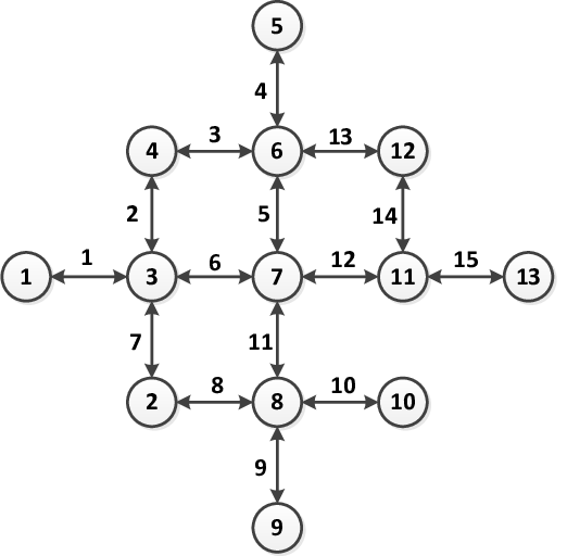
The second experiment involves a test problem introduced by Ramazani et al. [3]. It is based on a network with 13 nodes, 15 links and five junctions depicted in Fig. 5. The capacity and free-flow cost of network links are presented in Table 4. Assume six $(o,d)$ pairs $\{(1,9),(1,10),(1,13),(5,9),(5,10),(5,13)\}$ with demand $\{100,200,100,150,150,150\}$, the results of the equilibrium flows and the equilibrium path data of each $(o,d)$ pair are presents in Table 5 and Table 6, respectively. Table 5

References

- [1] T. L. Friesz, Transportation network equilibrium, design and aggregation: key developments and research opportunities, Transportation Research Part A: General 19 (1985) 413–427.
- [2] H. F. Wang, H. L. Liao, User equilibrium in traffic assignment problem with fuzzy n–a incidence matrix, Fuzzy sets and systems 107 (1999) 245–253.
- [3] M. Ghatee, S. M. Hashemi, Traffic assignment model with fuzzy level of travel demand: An efficient algorithm based on quasi-logit formulas, European Journal of Operational Research 194 (2009) 432–451.
- [4] R. Z. Farahani, E. Miandoabchi, W. Szeto, H. Rashidi, A review of urban transportation network design problems, European Journal of Operational Research 229 (2013) 281–302.
- [5] B. George, S. Kim, Spatio-temporal networks: An introduction, in: Spatio-temporal Networks, Springer, 2013, pp. 1–6.
- [6] J. E. Burrell, Multiple route assignment and its application to capacity restraint, in: Proceedings of Fourth International Symposium on the Theory of Traffic Flow.
- [7] R. B. Dial, A probabilistic multipath traffic assignment model which obviates path enumeration, Transportation research 5 (1971) 83–111.
- [8] H. Bar-Gera, Traffic assignment by paired alternative segments, Transportation Research Part B: Methodological 44 (2010) 1022–1046.
- [9] J. G. Wardrop, Road paper. some theoretical aspects of road traffic research., in: ICE Proceedings: Engineering Divisions, volume 1, Thomas Telford, pp. 325–362.
- [10] M. Beckmann, C. McGuire, C. B. Winsten, Studies in the Economics of Transportation, Technical Report, 1956.
- [11] T. L. Friesz, T. Kim, C. Kwon, M. A. Rigdon, Approximate network loading and dual-time-scale dynamic user equilibrium, Transportation Research Part B: Methodological 45 (2011) 176–207.
- [12] A. Chen, S. Ryu, X. Xu, K. Choi, Computation and application of the paired combinatorial logit stochastic user equilibrium problem, Computers & Operations Research 43 (2014) 68–77.
- [13] Z. Zhou, A. Chen, S. Bekhor, C-logit stochastic user equilibrium model: formulations and solution algorithm, Transportmetrica 8 (2012) 17–41.
- [14] T. Akiyama, H. Yamanishi, Travel time information service device based on fuzzy sets theory, in: Uncertainty Modeling and Analysis, 1993. Proceedings., Second International Symposium on, IEEE, pp. 238–245.
- [15] V. Henn, Fuzzy route choice model for traffic assignment, Fuzzy Sets and Systems 116 (2000) 77–101.
- [16] M. Ridwan, Fuzzy preference based traffic assignment problem, Transportation Research Part C: Emerging Technologies 12 (2004) 209–233.
- [17] T. Nakagaki, H. Yamada, Á. Tóth, Intelligence: Maze-solving by an amoeboid organism, Nature 407 (2000) 470–470.
- [18] T. Nakagaki, H. Yamada, A. Toth, Path finding by tube morphogenesis in an amoeboid organism, Biophysical chemistry 92 (2001) 47–52.
- [19] A. Adamatzky, Slime mold solves maze in one pass, assisted by gradient of chemo-attractants, NanoBioscience, IEEE Transactions on 11 (2012) 131–134.
- [20] T. Nakagaki, M. Iima, T. Ueda, Y. Nishiura, T. Saigusa, A. Tero, R. Kobayashi, K. Showalter, Minimum-risk path finding by an adaptive amoebal network, Physical review letters 99 (2007) 068104.
- [21] Y. Zhang, Z. Zhang, Y. Deng, S. Mahadevan, A biologically inspired solution for fuzzy shortest path problems, Applied Soft Computing 13 (2013a) 2356–2363.
- [22] X. Zhang, Z. Zhang, Y. Zhang, D. Wei, Y. Deng, Route selection for emergency logistics management: A bio-inspired algorithm, Safety Science 54 (2013b) 87–91.
- [23] A. Tero, S. Takagi, T. Saigusa, K. Ito, D. P. Bebber, M. D. Fricker, K. Yumiki, R. Kobayashi, T. Nakagaki, Rules for biologically inspired adaptive network design, Science 327 (2010) 439–442.
- [24] A. Adamatzky, M. Prokopenko, Slime mould evaluation of australian motorways, International Journal of Parallel, Emergent and Distributed Systems 27 (2012) 275–295.
- [25] A. Tero, R. Kobayashi, T. Nakagaki, A mathematical model for adaptive transport network in path finding by true slime mold, Journal of theoretical biology 244 (2007) 553–564.
- [26] M. Smith, The existence, uniqueness and stability of traffic equilibria, Transportation Research Part B: Methodological 13 (1979) 295–304.
- [27] L. A. Zadeh, Fuzzy sets, Information and Control 8 (1965) 338–353.
- [28] C. Yang, L. Bruzzone, F. Sun, L. Lu, R. Guan, Y. Liang, A fuzzy-statistics-based affinity propagation technique for clustering in multispectral images, Geoscience and Remote Sensing, IEEE Transactions on 48 (2010) 2647–2659.
- [29] P. K. Giri, M. K. Maiti, M. Maiti, Fuzzy stochastic solid transportation problem using fuzzy goal programming approach, Computers & Industrial Engineering 72 (2014) 160–168.
- [30] A. Azadeh, M. Moghaddam, M. Khakzad, V. Ebrahimipour, A flexible neural network-fuzzy mathematical programming algorithm for improvement of oil price estimation and forecasting, Computers & Industrial Engineering 62 (2012) 421–430.
- [31] H. Hu, Z. Li, A. Al-Ahmari, Reversed fuzzy petri nets and their application for fault diagnosis, Computers & Industrial Engineering 60 (2011) 505–510.
- [32] H. T. Nguyen, V. Kreinovich, B. Wu, G. Xiang, Computing Statistics Under Interval and Fuzzy Uncertainty: Applications to Computer Science and Engineering, Springer Publishing Company, Incorporated, 2011.
- [33] Y. Deng, W. Jiang, R. Y. Deng, Modeling contaminant intrusion in water distribution networks: A new similarity-based dst method, Expert Systems with Applications 38 (2011) 571–578.
- [34] A. Kauffman, M. M. Gupta, Introduction to Fuzzy Arithmetic: Theory and Application, Van Nostrand Reinhold, New York, 1991.
- [35] R. Ezzati, R. Saneifard, A new approach for ranking of fuzzy numbers with continuous weighted quasi-arithmetic means, Mathematical Sciences 4 (2010) 143–158.
- [36] R. E. Giachetti, R. E. Young, A parametric representation of fuzzy numbers and their arithmetic operators, Fuzzy Sets and Systems 91 (1997) 185–202.
- [37] S.-M. Chen, Fuzzy system reliability analysis using fuzzy number arithmetic operations, Fuzzy Sets and Systems 64 (1994) 31–38.
- [38] D. Guha, D. Chakraborty, A new approach to fuzzy distance measure and similarity measure between two generalized fuzzy numbers, Applied Soft Computing 10 (2010) 90–99.
- [39] S. Sadi-Nezhad, K. Khalili Damghani, Application of a fuzzy topsis method base on modified preference ratio and fuzzy distance measurement in assessment of traffic police centers performance, Applied Soft Computing 10 (2010) 1028–1039.
- [40] B. S. Gildeh, D. Gien, La distance-dp,q et le cofficient de corrlation entre deux variables alatoires floues, Actes de LFA 2001 (2001) 97–102.
- [41] I. Mahdavi, R. Nourifar, A. Heidarzade, N. M. Amiri, A dynamic programming approach for finding shortest chains in a fuzzy network, Applied Soft Computing 9 (2009) 503–511.
- [42] R. Hassanzadeh, I. Mahdavi, N. Mahdavi-Amiri, A. Tajdin, A genetic algorithm for solving fuzzy shortest path problems with mixed fuzzy arc lengths, Mathematical and Computer Modelling Article in Press, Corrected Proof (2011).
- [43] H. Ramazani, Y. Shafahi, S. Seyedabrishami, A fuzzy traffic assignment algorithm based on driver perceived travel time of network links, Scientia Iranica 18 (2011) 190–197.
- [44] T. A. Manual, Us bureau of public roads, Washington, DC 113 (1964).
- [45] Y. Deng, Y. Chen, Y. Zhang, S. Mahadevan, Fuzzy dijkstra algorithm for shortest path problem under uncertain environment, Applied Soft Computing 12 (2012) 1231–1237.
- [46] R. Hassanzadeh, I. Mahdavi, N. Mahdavi-Amiri, A. Tajdin, A genetic algorithm for solving fuzzy shortest path problems with mixed fuzzy arc lengths, Mathematical and Computer Modelling 57 (2013) 84–99.