Diffusion and bulk flow in phloem loading:
A theoretical analysis of the polymer trap mechanism for sugar transport in plants
Abstract
Plants create sugar in the mesophyll cells of their leaves by photosynthesis. This sugar, mostly sucrose, has to be loaded via the bundle sheath into the phloem vascular system (the sieve elements), where it is distributed to growing parts of the plant. We analyze the feasibility of a particular loading mechanism, active symplasmic loading, also called the polymer trap mechanism, where sucrose is transformed into heavier sugars, such as raffinose and stachyose, in the intermediary-type companion cells bordering the sieve elements in the minor veins of the phloem. Keeping the heavier sugars from diffusing back requires that the plasmodesmata connecting the bundle sheath with the intermediary cell act as extremely precise filters, which are able to distinguish between molecules that differ by less than 20% in size. In our modeling, we take into account the coupled water and sugar movement across the relevant interfaces, without explicitly considering the chemical reactions transforming the sucrose into the heavier sugars. Based on the available data for plasmodesmata geometry, sugar concentrations and flux rates, we conclude that this mechanism can in principle function, but that it requires pores of molecular sizes. Comparing with the somewhat uncertain experimental values for sugar export rates, we expect the pores to be only 5-10% larger than the hydraulic radius of the sucrose molecules. We find that the water flow through the plasmodesmata, which has not been quantified before, contributes only 10-20% to the sucrose flux into the intermediary cells, while the main part is transported by diffusion. On the other hand, the subsequent sugar translocation into the sieve elements would very likely be carried predominantly by bulk water flow through the plasmodesmata. Thus, in contrast to apoplasmic loaders, all the necessary water for phloem translocation would be supplied in this way with no need for additional water uptake across the plasma membranes of the phloem.
August 24, 2026
pacs
47.63.-b, 47.56.+r, 87.16.dpI Introduction
Leaves maintain an extremely delicate balance between water and sugar translocation to ensure the outflow and eventual evaporation of water from the xylem cells simultaneously with the inflow of water and sugar to the phloem cells nearby. Xylem and phloem are the two long distance pathways in vascular plants, where the former conducts water from the roots to the leaves and the latter distributes the sugar produced in the leaves. The sugar which is loaded into the sieve elements, the conducting cells of the phloem is generated in the chloroplasts of the mesophyll cells outside the bundle sheath, a layer of tightly arranged cells around the vascular bundle, which protects the veins of both xylem and phloem from the air present in the space between the mesophyll cells and the stomata. The latter are specialised cells, that control the air flow in and out of the leaf by adjusting the size of pores in the epidermis. The water which leaves the xylem is under negative pressure, up to bars have been reported [1], whereas the water in the phloem a few micrometers away is under positive pressure, typically around bars [2]. On the other hand, the sugar concentration is close to 0 in the xylem and up to 1 molar in the phloem, where the Münch mechanism [3] is believed to be responsible for the flow: the large sugar concentrations in the phloem cells of the mature “source” leaves will by osmosis increase the pressure and drive a bulk flow towards the various “sinks”, where sugar is used.
The water flow from the xylem has two important goals: most of it evaporates, presumably from the walls of the mesophyll cells, maintaining the negative pressures in the xylem necessary to draw water from the roots, but a small part of it passes across the plasma membranes into the mesophyll cells and takes part in the photosynthesis and the subsequent translocation of the sugars through the bundle sheath towards the sieve elements of the phloem. This loading process is not understood in detail, but several important characteristics are known and plants have been divided into rough categories [4] depending on their loading mechanisms. Many trees are so-called “passive loaders”, which means that the sugar concentration is largest in the mesophyll and decreases towards the sieve cells. This implies that sugar could simply diffuse from mesophyll cells to sieve elements without any active mechanism.
In other plants the concentrations are reversed, with the largest concentration occurring in the phloem, which then involves some active mechanism. An interesting class of plants is believed to make use of the so-called “active symplasmic” loading or “polymer trap” mechanism [4], which is illustrated in Fig. 1. Here high concentrations, and thus efficient sugar translocation in the sap, are achieved actively, by transforming the sucrose generated in the mesophyll and transported into the bundle sheath into heavier sugars, the oligosaccharides raffinose and stachyose, which are too large to diffuse back.
The flow into the phloem can follow two pathways, either through the symplasm (the interior of the cells) or through the apoplast (the space outside the plasma membranes, e.g., cell walls). In symplasmic loaders abundant plasmodesmata, i.e., membrane-surrounded channels through the cell walls, provide continuity of the loading pathway and therefore the sugar does not have to pass the plasma membranes as shown in Fig. 1. It has recently been pointed out that the polymer trap mechanism would require plasmodesmata with very specific filtering properties allowing sufficient amounts of sucrose to pass while blocking the heavier sugars [5].
We analyze this question in the present paper including both sugar diffusion and bulk water flow in our model without explicitly considering the chemical
reactions transforming the sucrose into the heavier sugars. We restrict the scope of our model to the part of the leaf where the loading of sugar into the phloem transport system takes place. We therefore only include one bundle sheath cell (BSC), intermediary cell (IC) and sieve element (SE) and their interfaces in our study. We also restrict the model to a steady-state situation in which flows, concentrations and pressures are constant. We derive and solve general equations for this setup and check their plausibility and implications with the help of the most complete set of measured values that we could find (for Cucumis melo).
The phloem cells in the leaf need water for sugar translocation and they need to build up sufficient pressure ( in Fig. 1) to generate efficient bulk movement of the phloem sap. On the other hand, the pressure cannot be too high in cells which are exposed to the xylem. Otherwise they would lose water across the water permeable plasma membrane towards the apoplast. If sugar is loaded only via diffusion without any significant water flow, the sieve element has to draw in the water from the surroundings across its plasma membrane. This requires a sufficiently low water potential in the phloem, i.e., a hydrostatic pressure significantly lower than the osmotic pressure . If, on the other hand, enough water flows along with the sugar through the plasmodesmata, i.e., symplasmically, the plant does not have to draw in water across the plasma membrane of the phloem cells (sieve element plus intermediary cells) and the hydrostatic pressure can therefore be greater, leading to more efficient vascular flow.
In the following we shall point out a likely scenario (see Sec. V.2), in which the polymer trap mechanism can function. We stress that this conclusion is based on very limited experimental information. There is a severe lack of precise knowledge on the anatomy of the plasmodesmata, the precise sugar concentrations (taking sufficient account of the distribution of the sugars inside the compartments of the cells) and as the most severe problem, an almost total lack of pressure measurements. The latter reflects the fact that determination of the pressure in a functioning (living) phloem is at present not feasible.
From our analysis, however, some important features of this special and fascinating loading mechanism has become clear. Analysing simple equilibrium configurations with the use of irreversible thermodynamics (Kedem-Kachalsky equations) and the theory of hindered transport, we show that diffusion can in fact, despite claims to the contrary [5], be sufficient to load the sucrose through narrow plasmodesmata into the phloem of a polymer trap plant, while efficiently blocking the back flow of larger sugars. The simultaneous water flow can also be of importance not only to support the sugar flux but also to achieve advantageous pressure relations in the leaf and thus to preserve the vital functions of the strongly interdependent phloem and xylem vascular systems. We show that the bulk water entering the symplasm of pre-phloem cells already outside the veins can effectively suffice to drive the Münch flow, although the same flow does only contribute a minor part to the loading of sugar into the intermediary cells of the phloem.
II The polymer trap model

The polymer trap loading mechanism was postulated for angiosperm taxa, for example, cucurbits, and is shown in Fig. 1.
Most of the concrete values which are used in our calculations, i.e., the sugar concentrations in the cells of the loading pathway [6], the surface and interface areas of the cells [7], and the total leaf sugar export [8], were measured in muskmelon (Cucumis melo). The cytosolic concentration of sucrose is around [6] in the mesophyll and bundle sheath cells (BSCs) taking into account the intracellular compartmentation. Sucrose passes symplasmically through narrow plasmodesmata (PDs) into the companion cells of the phloem, which are called intermediary cells (ICs) in this special loading type. In the ICs the sucrose is converted to larger oligomers, also called raffinose family oligosaccharides (RFOs), which pass through relatively wide PDs into the sieve element (SE). The tetrasaccharide stachyose is the most abundant sugar oligomer in the phloem of Cucumis melo. The sucrose and stachyose concentrations in the phloem cytosol, i.e., in the cell sap outside of the vacuole, were measured to be about and , respectively [6]. These two sugars represent together about of the total sugar concentration in the phloem, which, with a value of , is more than twice as large as the concentration in the bundle sheath cytosol [6].
On the contrary, almost no RFOs have been found outside the SE-IC complex, and since no evidence for active sucrose transporters in the bundle sheath membranes of RFO-transporting plants have been found, it seems that the narrow plasmodesmatal pores in the BSC-IC interface must provide the delicate filtering effect letting the smaller sucrose molecules pass from the bundle sheath while retaining the oligomers in the phloem [4].
For this task, the effective pore widths must be similar to the diameters of the sugar molecules i.e., around . Such small widths seem at least not in conflict with evidence from electron microscopy, where parts of the plasmodesmata found in the IC wall look totally obstructed [9], but where one can hardly resolve patterns of sizes below . Schmitz et al. measured the total export rate in leaves of Cucumis melo [8], from which a sugar current density across the BSC-IC interface can be calculated [5].
The explanation of the functioning of the polymer trap given by Turgeon and collaborators [4] is that the sucrose diffuses along a downhill concentration gradient into the phloem while the oligomers, which are synthesized by enzymatic reactions at this location, are blocked by the specialized narrow PDs in the IC wall from diffusing back into the bundle sheath. This simple picture was questioned by Liesche and Schulz [5], who considered quantitatively the hindered diffusion across the BSC-IC interface. In the present paper, we present an extended model, relating the transport coefficients to the structure and density of PDs in the cellular interfaces, and including explicitly the water flow. Based on the available experimental data, we show that pure diffusion can create a large enough sugar export in Cucumis melo while blocking the oligosaccharides, but since the pores are of the dimension of the sugar molecules, osmotic effects across the cell interfaces are unavoidable and probably important. Thus, the resulting water flows may be crucial for building up the bulk flow in the phloem vascular system. We calculate the hydrostatic pressures created in the cells, and to compute a possible water intake across the cell membranes, we have to compare the resulting water potentials to that of the apoplast outside the cell membranes. We expect the pressures in the apoplast to be close to the (negative) values in the xylem, which are unfortunately not known for this particular species. However, we assume the value in musk melon to be close to that in maize, which has a typical xylem pressure of around [10]. The (positive) so-called turgor pressure for well-hydrated living cells should be large enough to keep the fairly elastic plasma membrane tight against the rigid cell wall. Since there are, as far as we know, no data available for the leaf cell pressures in Cucumis melo we assume them to be larger than and close to the ambient pressure similar to the mesophyll turgor pressures measured in Tradescantia virginiana [11]. We use the lower limit as a reasonable value for the bundle sheath pressure in our numerical calculations. With this assumption the pressure in the phloem thus builds up to values of close to 10 bars, which is a typical value quoted for the phloem pressure [12, 2].
II.1 Transport equations for the polymer trap model
Our model (see Fig. 1) considers diffusion and bulk flow through the plasmodesmata of the BSC-IC and IC-SE cell interfaces and furthermore takes into account a possible osmotic water flow across the IC-plasma membrane. For simplicity we assume here that, in the IC, two sucrose molecules are oligomerized to one tetrasaccharide, corresponding to a stachyose molecule in Cucumis melo. The volume and sugar flows across the two cell interfaces can be written using the Kedem-Katchalsky equations [13] for membrane flows in the presence of multiple components. The volumetric water flow rates (measured, e.g., in ) into and out of the IC can be expressed as
| (1) | ||||
| (2) | ||||
where the subscripts number the cells in the sequence BSC, IC, SE, and . The superscripts denote the molecule species, sucrose (s) and oligomer (o). The water potentials are defined as . Note that the water can flow through the plasmodesmata from a lower to a higher water potential because of the different osmotic effects of the sugar species. The coefficients are the bulk hindrance factors , where is the reflection coefficient used by Kedem and Katchalsky. Thus, if for a given molecule, it cannot get through the membrane and creates a full osmotic pressure, while means that the molecule passes as easily as the water molecules. We use the universal gas constant and the absolute temperature .
The corresponding sugar flow rates (e.g., in ) can then be written as
| (3) | ||||
| (4) |
Here is a diffusion coefficient related to the diffusive mobility used by Kedem and Katchalsky as . is an interfacial area and is the diffusion distance, i.e., the thickness of the intermediary cell wall. The two terms in describe, respectively, the advective contribution (proportional to ) and the diffusive one (proportional to the concentration differences). The interface coefficients are computed in the next section, based upon the geometry of the PDs.
If we introduce average interface coefficients and with the sucrose and oligomer proportions in the phloem, the expressions (2) and (4) for the outflows can be simplified to
| (5) | ||||
| (6) |
where we assume that the sucrose and oligomer proportions are the same in the SE and the IC. There might also be an osmotic water flow across the IC membrane, which builds a connection to the apoplast, where we expect a (negative) hydrostatic pressure , probably close to the xylem pressure. This trans-membrane flow can be written using the permeability coefficient and the van’t Hoff equation for an ideally semi-permeable IC membrane as
| (7) |
For a water flow into the intermediary cell the water potential has to be less (more negative) than the pressure in the apoplast. The flows into and out of the IC are related by conservation laws for water and sugar in the form
| (8) | ||||
| (9) |
where Eq. (9) is derived from the mass conservation of sugar molecules in the intermediary cell with the molar masses related by used in our approximate model.
III Estimates of the coefficients and concentrations

| Variable | Measured as | Value | Unit | Reference |
|---|---|---|---|---|
| Interface area between IC and BSC | [7] | |||
| Interface area between IC and SE | [7] | |||
| Surface area of the IC | [7] | |||
| Hydrodynamic radius of sucrose from 3D-model | [5] | |||
| Hydrodynamic radius of stachyose from 3D-model | [5] | |||
| Free cytosolic diffusion coefficient for sucrose | [14] | |||
| Free cytosolic diffusion coefficient for stachyose | [15] | |||
| Shape factor for hydrated sucrose molecules | ||||
| Shape factor for hydrated stachyose molecules | ||||
| Dynamic viscosity of cytosol | [5] | |||
| Half-slit width of PDs in the IC wall | [9, 16] | |||
| Half-slit width of ”normal” PDs | [16] | |||
| Average radius of PDs in plant cell walls | [9, 16] | |||
| Thickness of the IC wall | [7] | |||
| Density of PDs in the IC wall | [7] | |||
| Cytosolic sucrose concentration in mesophyll and bundle sheath | [6] | |||
| Total cytosolic sugar concentration in the IC-SE complex | [6] | |||
| Cytosolic sucrose concentration in IC-SE complex | [6] | |||
| Sucrose concentration difference between BSC- and IC-cytosol | [5, 6] | |||
| Hydrostatic pressure in the bundle sheath | [11] | |||
| Xylem and apoplast pressure (from maize) | [10] | |||
| Sugar current density through BSC-IC interface, from total leaf export rate | [8] |
estimated from the given references.
The cell interfaces are modeled as porous membranes. From detailed electron microscopic investigations [9, 7] the PDs at this specific interface are generally branched towards the IC. However, the detailed substructure is not known, in particular the shape and area of the cytoplasmic sleeve connecting the cytosol of the cells.
For our modeling we simplify these channels as circular slits (see Fig. 2), as suggested in Ref. [17], with average radius , half-width , and length equal to the thickness of the part of the cell wall belonging to the IC.
From the slit geometry together with the density of plasmodesmata and the interface areas (see Table 1) the interface coefficients can be calculated using the hindrance factors and for diffusion and convection in narrow pores, which were recently analyzed by Deen and Dechadilok [18]. For spherical particles these hindrance factors have been estimated as polynomials in the relative solute size . The following expressions are valid for (H) and (W),
| (10) | ||||
| (11) |
For the solute should be totally blocked by the plasmodesmatal pores. In this case both hindrance factors are set to zero. Plots of the hindrance factors as functions of are shown in Fig. 3.

The bulk hindrance factor enters our equations directly as one of the three interface coefficients. The diffusive hindrance factor is used together with the pore covering fraction to compute the effective diffusion coefficients appearing in (3) and (4) as
| (12) |
Here the covering fraction is given as the ratio of free slit-space to total cell-interface area, i.e.,
| (13) |
where is the density of plasmodesmata in the IC wall, and the unobstructed sleeve is assumed to be very narrow (). The free diffusion coefficient of the respective solutes in cytosol can be written using the Einstein relation for diffusing spherical molecules as
| (14) |
with the hydrodynamic radii of the solutes, the cytosolic viscosity and the Boltzmann constant related to the universal gas constant by the Avogadro constant .
The shape factor accounts for the deviation from the Einstein relation primarily due to the non spherical shape of the molecule. In our modeling we use a three-dimensional (3D) structural model to compute the radii for hydrated molecules [5] and thus include shape factors of the order of unity (see table 1).
The permeability coefficient for the BSC-IC and IC-SE-interface is estimated using a pressure driven Poiseuille-flow through narrow rectangular channels of height and width , where , i.e.
| (15) | ||||
| (16) |
The cytosolic viscosity is estimated with a value twice as large as the viscosity of water, i.e., . The characteristic cell-wall thickness as well as the plasmodesmata radius have been estimated from TEM-images [7, 19]. Based on the measurements by Volk et al., the density of plasmodesmata in the IC wall is fixed to a value of around [7]. For the BSC-IC interface we assume that the PDs are very narrow and have a half-width between the hydrodynamic radius of sucrose and of stachyose , since stachyose should be totally blocked from going back to the bundle sheath. We shall choose as a standard value since it is the largest value for which we are certain that (see, however, the final section on raffinose hindrance). The hydrodynamic radii and have been computed using the 3D-structural models of hydrated sucrose and stachyose molecules accounting in particular for the cylindrical molecule forms [5]. For the IC-SE interface, the PDs are wider and we use a “normal” slit-width [16]. The interface coefficients for this configuration are listed in table 2.
The sucrose and total sugar concentrations in the IC are fixed to the values and , respectively (see Table 1), based on the measured concentrations from Ref. [6].
| Coefficient | Value | Unit |
|---|---|---|
IV Dimensionless equations and their solution
| Variable | Scaling factor | Value |
|---|---|---|
| () | ||
| () | ||
To nondimensionalize we scale the used variables with the factors stated in Table 3 based on the concentration in the BSC and the properties of the BSC-IC interface. The dimensionless flows can be written as
| (17) | ||||
| (18) | ||||
| (19) | ||||
| (20) | ||||
| (21) |
The dimensionless sugar inflow corresponding to the experimentally determined sugar current density [8] in Cucumis melo is
| (24) |
The scaled permeability and effective diffusion coefficients take the form
| (25) | ||||
| (26) | ||||
| (27) |
Here the definitions from Sec. III and the scaling factors from Table 3 were used, and the relative solute size in the slits of half-width is defined as . The expression can be understood as the average number of sucrose molecules in the BSC in a small volume of the dimension of the sugar molecules. Inserting the dimensionless coefficients in the scaled flows, these can be rewritten as
| (28) | ||||
| (29) | ||||
| (30) | ||||
| (31) | ||||
| (32) | ||||
| (33) |
The bar over a variable always denotes an average quantity, calculated with the proportions of the two different sugars in the phloem, e.g., using the proportions and of sucrose and oligomer molecules in the phloem.
We can use, for example, and as independent variables and calculate the other quantities. The sucrose and oligomer concentrations in the intermediary cell can be calculated from the concentration difference between the BSC and the IC, and the oligomer proportion in the phloem using e.g., , , . The concentration in the sieve element can then be determined from the volume and sugar conservation equations (22) and (23) with the use of expressions (30) and (32) for the sugar flow rates, i.e.
| (34) |
Finally, using the expressions for the water flows (28), (29), and (19), the water potentials , , and and corresponding hydrostatic pressures inside and outside the cells of the loading pathway can be calculated (with the interface coefficients from Table 2 and the geometry as fixed in Table 1) as
| (35) | ||||
| (36) | ||||
| (37) |
V Special cases
V.1 Pure Diffusion
In this subsection we first investigate whether pure diffusion through plasmodesmata can transport enough sugar into the phloem, and, subsequently, whether this special case with no bulk flow through the plasmodesmata represents a likely loading situation in real plants. Assuming that the sucrose is transported into the IC by pure diffusion without a supporting bulk flow, we get
| (38) |
This is in agreement with Fick’s first law of diffusion. Taking gives . The sugar current depends on the half-slit width of the PDs in the BSC-IC interface through the relative solute size , which also appears as variable in the diffusive hindrance factor .
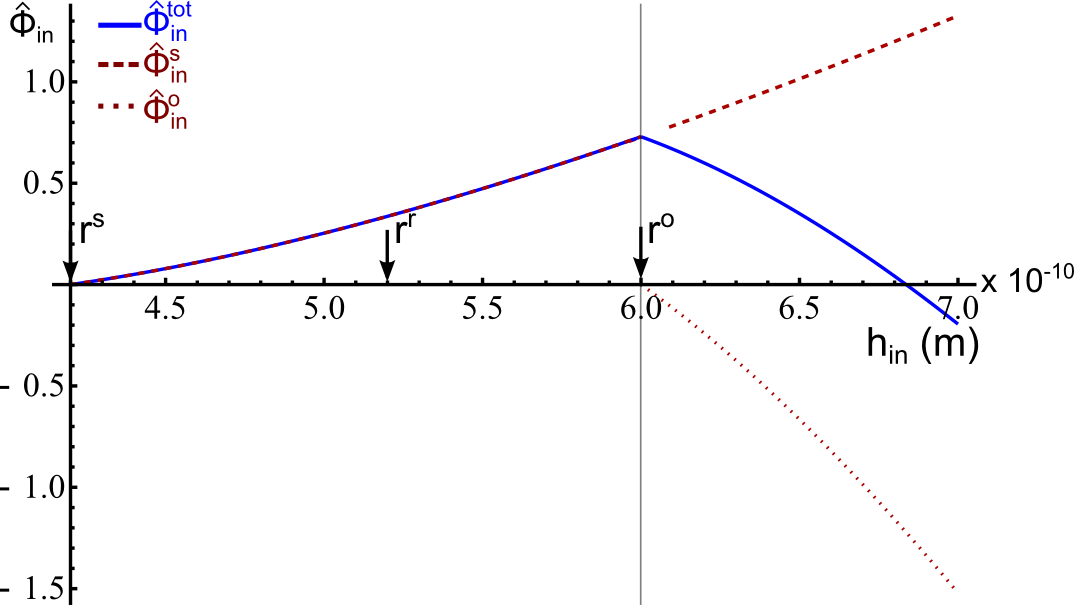
Figure 4 shows that even for slits which are only slightly larger than the oligomers, the back flow into the bundle sheath due to diffusion would exceed the sucrose flux in the opposite direction.
With our standard half-slit width of equal to the hydrodynamic radius of the stachyose molecules, corresponding to a relative sucrose size of , the tetrasaccharides in our model are blocked completely. For the sucrose flow rate we get , which is about 30 times larger than the experimental value from Ref. [8]. This shows that, in Cucumis melo, diffusion through the narrow plasmodesmatal pores can be sufficient to achieve the measured sugar current into the phloem, and in fact the large value that we obtain probably means that the pores are even narrower than the size of the stachyose molecules. Indeed, the pores also have to be able to block the back flow of raffinose, which is around 10 % smaller than stachyose. We discuss that in Sec. V.4 .
We found that pure diffusion is sufficient to export enough sugar into the phloem of RFO-transporting plants. On the other hand, the long-distance transport in the phloem system is based on a bulk flow for which water has to enter the symplasm at some point. Since in this special case we ruled out any bulk flow through the plasmodesmata between BSC and IC, the water has to go across the membrane of either the intermediary cell or the sieve element. We now calculate the pressures, concentrations, and water potentials in these cells to see if this is a possible and even advantageous situation for the plant, i.e., if the water potentials are low enough for water from the xylem to be drawn in. The condition of purely diffusive sugar loading implies that the hydrostatic and osmotic pressure differences across the BSC-IC interface must be balanced in order to achieve zero bulk flow. From this boundary condition, i.e., , the water potential and hydrostatic pressure in the intermediary cell can be calculated for a fixed potential in the bundle sheath. With Eq. (35) is reduced to
| (39) |
For a water potential of , corresponding to in the bundle sheath, a value results in the IC which corresponds to . To avoid inflow of water from the BSC, the intermediary cell thus has to build up a large hydrostatic pressure of . If the water needed in the phloem enters as across the membrane of the intermediary cell, the pressure in the apoplast has to be larger than the water potential in the IC, i.e., . As mentioned above we assume the xylem pressure to be around [10], and thus such a water uptake would not be feasible. For pressures bar this conclusion is even more justified.
Now we consider the case where the flow through the PDs into the sieve element also vanishes, i.e., . In this situation, the water from the xylem must flow in across the membrane of the sieve element. The concentration in the SE can be calculated with Eq. (34), which simplifies for pure diffusion at both interfaces to
| (40) |
The resulting concentration in the sieve element is lower than the IC-sugar concentration because a downhill gradient to the SE is essential for diffusion. The water potential is calculated with Eq. (36) for zero water outflow as
| (41) |
and we obtain a value of corresponding to and . To generate osmotic water flow into the SE, the xylem pressure has to be larger than , i.e., , which makes it even more difficult for the water to flow directly into the sieve element than into the IC. Thus the water potential in both of the phloem cells (IC and SE) will probably be too high to allow sufficient water intake across the cell membrane from the xylem system. Furthermore pure diffusion across the IC-SE interface requires that the sugar concentration decreases into the SE [as seen in Eq. (40)], which presumably is a disadvantage for efficient sugar translocation. In both respects the situation improves, when we allow for water flow through the PD pores in the BSC-IC interface as we show below.
V.2 Equal concentrations in SE and IC
The general case with both diffusion and water flow across both cell interfaces is complicated as seen, for example, from Eq. (34), and one has to deal with many unknown variables, mainly pressures, bulk flows, and the SE concentration. In this subsection we shall therefore treat the special case, where the concentrations in the intermediary cell and sieve element are equal, i.e., , which is likely due to the well connected IC-SE complex. Compared to pure diffusion into the SE this has the advantage, that the concentration of sugar in the phloem sap is higher and therefore the sugar flow will be larger. As a consequence of the equal concentrations in the phloem, the sugar from the IC will be transported by pure bulk flow from the intermediary cell into the sieve element. Using (30) and (32), the sugar flows are then expressed as
| (42) | ||||
| (43) |
Using the volume conservation (22) we can determine the volume flow and sugar flow from the sugar conservation (23) with a given trans-membrane flow as functions of the concentration in the phloem, i.e.,
| (44) | ||||
| (45) |
Here the proportions and and consequently the average bulk hindrance factor at the IC-SE interface also depend on . The corresponding inflows are subsequently determined by the conservation laws. The higher we choose the oligomer concentration for a fixed sucrose concentration the lower are the resulting flows, approaching the limits
| (46) | ||||
| (47) |
The contribution of the bulk flow to the inflowing sugar current decreases for high IC-concentrations, if there is no runoff of pure water from the IC into the apoplast that would prevent the dilution of the concentrated phloem solution. Since the diffusive contribution stays constant due to the fixed sucrose gradient, the total sugar inflow decreases together with the water flow for a more concentrated phloem solution as seen in Fig. 5.
We do not know values for the permeability of the plasma membranes on the loading pathway. Depending on the abundance of aquaporins, i.e., water-conducting proteins, it can vary by several orders of magnitude between and as measured by Maurel in plant cells [20]. We assume here, however, that the permeability of the IC-plasma membrane is much smaller than the permeabilities of the plasmodesmata, and we thus neglect in the following. For this case, Fig. 5 shows the behavior of the volume and sugar flows and as functions of as in Eqs. (44) and (45). For the measured IC concentration of in muskmelon [6] the bulk flow contributes to the sugar inflow only by . Also for , we have and the water potentials in the phloem can then be determined as
| (48) | ||||
| (49) |
For the concentrations in Cucumis melo and a bundle-sheath pressure of , the resulting values in the phloem are and corresponding to dimensional values and for the potentials and and for the hydrostatic pressures.

V.3 The loading unit as a part of the phloem
So far our modeling has not taken into account that the sieve elements are part of the phloem vascular system, and that sap is therefore transported from one sieve element to the next along the phloem vasculature. The pressure drop between the sieve elements needed for this flow is very small compared to the pressure drops across the PDs, which we have been considering so far, since the sieve elements and even the pores in the sieve plates are several orders of magnitude wider. Thus the sieve elements all probably have roughly the same pressures and concentrations. If we also suppose that there is no direct water exchange between the sieve elements and the apoplast, the sugar and water, which is loaded into the sieve elements, should have those same concentrations. The simplified flow in the last subsection, where we assumed equal sugar concentrations in the IC and SE and thus pure bulk advection through the IC-SE interface, would then be impossible, since it would result in the dilution of the phloem sap due to the different hindrances of the sugars and the water in the plasmodesmata. To find an appropriate condition, we denote the sugar flow rate from along the sieve tube (i.e., from one sieve element to the next) by and the amount provided by each IC as . If the concentration in the sieve element (of some solute) is , the sugar flow is related to the water flow rate simply by and the condition described above would then amount to , where is the flow rate of this particular solute across the IC-SE interface.
With no direct water exchange between the sieve element and the xylem, . Thus the conservation laws (23) and (22) result in the following equations, where at the IC-SE interface the sucrose and oligomer flux rates are both conserved and can therefore be treated separately, i.e.,
| (50) | ||||
| (51) | ||||
| (52) |
Here the dimensionless forms of (3) and (4) of the sugar in and out flow rates are used with . The average Eq. (21) with and can not be employed here, since the sugar ratios in the SE are in general not equal to in the IC. From these equations the SE concentrations and can be expressed as
| (53) |
Depending on the SE concentration will take a value between in the case of a very high advective contribution at the IC-SE interface, and for a very high diffusive contribution. The bulk flow can be determined from (50), (51), and (52) with . Using the specific values from Table 1, the resulting SE concentrations in Cucumis melo would then be and so that the total SE concentration lies as expected between and . The bulk contributions to the sugar flow rate at the different interfaces are then calculated with
| (54) | ||||
| (55) |
Thus the advective flow from the intermediary cell into the sieve element in this case contributes about 62 % to the overall sugar outflow while at the BSC-IC interface the bulk contribution would merely be 14 %. Furthermore the water potentials become (IC) and (SE) [using Eqs. (35) and (36)], and the pressures are and . So we believe that we have a consistent picture, where all the water necessary for the sap translocation in the phloem is provided together with the sugar through the plasmodesmata with no further need of osmotic water uptake.
V.4 Diffusion of raffinose
Up to this point, we have treated the oligosaccharides as one species with properties largely determined by stachyose, the one present in largest concentrations. This treatment presumably gives good estimates for the transport rates and water flux, but we still have to account for the fact that raffinose, which is smaller than stachyose, does not diffuse back into the bundle sheath. The transport of raffinose would be given as
| (56) |
where we have used the average raffinose concentration between BSC and IC in the advection term. Here we assume that the bulk water flow is still given by Eq. (28) used above, i.e.,
| (57) |
and we investigate whether the bulk flow is sufficient to block the diffusion of raffinose, which would mean that is actually positive. With the coefficients characterizing the movement of raffinose denoted by the superscript , we get
| (58) |
where we have neglected , which is typically less than or equal to 0. Using the raffinose radius from a 3D-structure model [5], the half-slit width as above and the measured free diffusion coefficient [21] in cytosol (half of the value in water) with we find and thus meaning that the bulk flow cannot block the back diffusion of the intermediate sized raffinose molecules.
Thus, to avoid the diffusion of raffinose back into the bundle sheath we need a half-slit width, which is very close to the radius of the raffinose molecules, denoted by above. Since these molecules are not spherical, the relevant size depends strongly on how it is defined and/or measured, and thus the hydrodynamic radius of raffinose can vary between values 10% and 20% above that of the sucrose molecules. In addition the corresponding value of is at the limit (or above) of the range of validity of the hindrance factors, so all in all our results will be somewhat uncertain. Using the value from 3D-modeling [5] gives for the sucrose molecules. Using this value in our equations does not change the qualitative features of the solutions obtained above (see Fig. 4). In this case, using Eq. (38), the sugar current would still be larger than the measured value (14 times larger instead of 30 times larger with the half-slit width ). Taking the values for the sucrose radius and as half-slit width directly from the Einstein relation [5] gives us , and in this case we are above the stated range of validity of . If we use the expressions (10) and (11) we get and . Using again Eq. (38) with , we obtain
| (59) |
which is still about three times the measured value 0.025. To get down to the experimental value we have to decrease the half-slit width below to , i.e., .
VI Conclusion
We have analyzed the feasibility of the polymer trap loading mechanism (active symplasmic loading) in terms of the coupled water and sugar movement through the plasmodesmata in the cellular interfaces leading from the bundle sheath to the phloem. We used the Kedem-Katchalsky equations and model the pores in the cell interfaces as narrow slits. This allowed us to compute the membrane coefficients using results on hindered diffusion and convection, and to check whether they can act as efficient filters, allowing sucrose to pass, but not raffinose and stachyose, synthesized in the intermediary cells. Based on the very limited available data for plasmodesmata geometry, sugar concentrations and flux rates, we conclude that this mechanism can in principle function, but, since the difference in size between raffinose and sucrose is only 10-20%, we are pressing the theories for hindered transport to the limit of (or beyond) their validity. We find that sugar loading is predominantly diffusive across the interface separating the bundle sheath from the phloem. However, the sugar translocation into the sieve tube, where the vascular sugar transport takes place, can be dominated by advection (bulk flow). This allows the plant to build up both the large hydrostatic pressure needed for the vascular sugar transport and the high concentration needed to make this transport efficient. This is possible because the water uptake to the sieve tubes happens directly through the plasmodesmata instead of through aquaporins in the cell membranes of the phloem. Thus, the water in the phloem has to be taken up across the plasma membranes of the pre-phloem pathway, e.g. the bundle sheath cells. As mentioned earlier, the experimental data available for these plants are very limited. It would be of great importance to have more information on the concentrations and pressures in the cells as well as the diffusivities across the important interfaces. It would also be of importance to extend the analysis of the sugar translocation all the way back to the mesophyll cells, where it is produced.
Acknowledgements
We are grateful to the Danish Research Council Natur og Univers for support under the grant 12-126055.
References
- [1] P. F. Scholander, E. D. Bradstreet, E. A. Hemmingsen, and H. T. Hammel, Science 148, 339 (1965).
- [2] L. Taiz and E. Zeiger, Plant Physiology, 3rd ed. (Sinauer Associates, Inc., Sunderland, MA, USA, 2002).
- [3] E. Münch, Die Stoffbewegungen in der Pflanze (Fischer, Jena, 1930).
- [4] E. A. Rennie and R. Turgeon, PNAS 106, 14162 (2009).
- [5] J. Liesche and A. Schulz, Front. Plant Sci. 4, 207 (2013).
- [6] E. Haritatos, F. Keller, and R. Turgeon, Planta (Heidelberg) 198, 614 (1996).
- [7] G. Volk, R. Turgeon, and D. Beebe, Planta (Heidelberg) 199, 425 (1996).
- [8] K. Schmitz, B. Cuypers, and M. Moll, Planta (Heidelberg) 171, 19 (1987).
- [9] G. D. Fisher, Planta (Heidelberg) 169, 141 (1986).
- [10] M. T. Tyree and M. H. Zimmermann, Xylem Structure and the Ascent of Sap (Springer, Heidelberg, 2002).
- [11] U. Zimmermann, D. Huesken, and E.-D. Schulze, Planta (Heidelberg) 149, 445 (1980).
- [12] P. Nobel, Plant Physiology, 2nd ed. (Academic Press, San Diego, 1999).
- [13] O. Kedem and A. Katchalsky, Biochim. Biophys. Acta 27, 229 (1958).
- [14] P. Henrion, Trans. Faraday Soc. 60, 72 (1964).
- [15] L. Craig and A. Pulley, Biochem. 1, 89 (1962).
- [16] A. G. Roberts and K. J. Oparka, Plant Cell Environ. 26, 103 (2003).
- [17] E. Waigmann, A. Turner, J. Peart, K. Roberts, and P. Zambryski, Planta (Heidelberg) 203, 75 (1997).
- [18] P. Dechadilok and W. M. Deen, Ind. Eng. Chem. Res. 45, 6953 (2006).
- [19] C. E. J. Botha, B. J. Hartley, and R. H. M. Cross, Ann. Botany (London) 72, 255 (1993).
- [20] C. Maurel, Annu. Rev. Plant Biol. 48, 399 (1997).
- [21] P. Dunlop, JOURNAL OF PHYSICAL CHEMISTRY 60, 1464 (1956).