跳到论文正文
W Papers独立论文阅读器 arXiv:1406.1396 论文正文 计算阅读时间 · 0%
引用这篇论文根据当前论文元数据生成,正式投稿前建议核对。


License: arXiv.org perpetual non-exclusive license
arXiv:1406.1396v3 [math.PR] 02 Oct 2014

A rate of convergence for the circular law for the complex Ginibre ensemble

Elizabeth S. Meckes and Mark W. Meckes Address: Department of Mathematics, Case Western Reserve University, 10900 Euclid Ave., Cleveland, Ohio 44106, U.S.A. Email address: elizabeth.meckes@case.edu Address: Department of Mathematics, Case Western Reserve University, 10900 Euclid Ave., Cleveland, Ohio 44106, U.S.A. Email address: mark.meckes@case.edu
Résumé.

Nous établissons des vitesses de convergence pour la loi du cercle de l’ensemble de Ginibre complexe. Plus précisément, nous donnons des bornes supérieurs pour les distances de Wasserstein d’ordre pp entre la mesure spectrale empirique de l’ensemble de Ginibre complexe normalisée et la mesure uniform du disque, dans l’espérance et presque sûrement. Si 1≤p≤21\leq p\leq 2, les bournes sont de la taille n−1/4n^{-1/4}, à des facteurs logarithmiques.

1. Introduction

Consider an n×nn\times n random matrix GnG_{n} with i.i.d. standard complex Gaussian entries; put slightly differently, GnG_{n} is a random element of the set of n×nn\times n matrices over ℂ\mathbb{C}, whose distribution has density proportional to e−tr⁡(G​G∗)e^{-\tr(GG^{*})}. The random matrix GnG_{n} is said to belong to the complex Ginibre ensemble. Although this ensemble was introduced by Ginibre [7] without any particular application in mind, the eigenvalues of GnG_{n} have since been used to model a wide variety of physical phenomena; see in particular [6] and [10] for references.

The central result about the asymptotic behavior of the eigenvalues of GnG_{n} is the famous circular law. Let μn\mu_{n} denote the empirical spectral measure of 1n​Gn\frac{1}{\sqrt{n}}G_{n}; that is,

μn=1n​∑k=1nδλk,\mu_{n}=\frac{1}{n}\sum_{k=1}^{n}\delta_{\lambda_{k}},

where λ1,…,λn\lambda_{1},\dots,\lambda_{n} are the eigenvalues of 1n​Gn\frac{1}{\sqrt{n}}G_{n}. The circular law states that when n→∞n\to\infty, μn\mu_{n} converges in some sense to the uniform measure ν\nu on the unit disc D:={z∈ℂ||z|≤1}D:=\left\{z\in\mathbb{C}\mathrel{}\middle|\mathrel{}\left|z\right|\leq 1\right\}. This was first established by Mehta [12], who showed that the mean empirical spectral measure 𝔼​μn\mathbb{E}\mu_{n} converges weakly to ν\nu. A large literature followed, which established the circular law for more general random matrix ensembles, and for stronger forms of convergence, culminating in the recent proof by Tao and Vu [18] of the circular law for random matrices with i.i.d. entries with arbitrary entries with finite variance, in the sense of almost sure weak convergence. The reader is referred to the survey by Bordenave and Chafaï [3] for further history and related results.

The main results of this paper give rates of convergence for the circular law for the complex Ginibre ensemble GnG_{n}, both in expectation and almost surely.

Theorem 1.

There is a constant C>0C>0 such that for all n∈ℕn\in\mathbb{N} and all p≥1p\geq 1,

𝔼​Wp​(μn,ν)≤C​max⁡{pn1/4,(log⁡nn)12​p},\mathbb{E}W_{p}(\mu_{n},\nu)\leq C\max\left\{\frac{\sqrt{p}}{n^{1/4}},\left(\frac{\log n}{n}\right)^{\frac{1}{2p}}\right\},

where Wp​(μ,ν)W_{p}(\mu,\nu) denotes the LpL_{p}-Wasserstein distance between probability measures μ\mu and ν\nu.

In particular, in the most widely used Wasserstein metrics, namely p=1,2p=1,2, we have

𝔼​W1​(μn,ν)≤Cn1/4and𝔼​W2​(μn,ν)≤C​(log⁡nn)14.\mathbb{E}W_{1}(\mu_{n},\nu)\leq\frac{C}{n^{1/4}}\qquad\mbox{and}\qquad\mathbb{E}W_{2}(\mu_{n},\nu)\leq C\left(\frac{\log n}{n}\right)^{\frac{1}{4}}.
Theorem 2.

For each p≥1p\geq 1 there is a constant Kp>0K_{p}>0 such that with probability 11, for sufficiently large nn,

Wp​(μn,ν)≤Kp​log⁡nn1/4W_{p}(\mu_{n},\nu)\leq K_{p}\frac{\sqrt{\log n}}{n^{1/4}}

when 1≤p≤21\leq p\leq 2, and

Wp​(μn,ν)≤Kp​(log⁡nn)1/2​pW_{p}(\mu_{n},\nu)\leq K_{p}\left(\frac{\log n}{n}\right)^{1/2p}

when p>2p>2.

Recall that for any p≥1p\geq 1, the LpL_{p}-Wasserstein distance between two probability measures μ\mu and ν\nu on ℂ\mathbb{C} is defined by

Wp​(μ,ν)=(infπ∈Π⁡(μ,ν)∫|w−z|p​𝑑π​(w,z))1/p,W_{p}(\mu,\nu)=\left(\inf_{\pi\in\Pi(\mu,\nu)}\int\left|w-z\right|^{p}\ d\pi(w,z)\right)^{1/p},

where Π⁡(μ,ν)\Pi(\mu,\nu) is the set of all couplings of μ\mu and ν\nu; i.e., probability measures on ℂ×ℂ\mathbb{C}\times\mathbb{C} with marginals μ\mu and ν\nu (see, e.g., [19]).

A few related results have appeared previously. In [17, Section 14], Tao and Vu sketched an argument giving an almost sure convergence rate for the empirical spectral measure of a random matrix 1n​Mn\frac{1}{\sqrt{n}}M_{n} with i.i.d. entries with a finite moment of order 2+ε2+\varepsilon. The convergence in this case was in Kolmogorov distance (sup-distance between bivariate cumulative distribution functions), and the rate is of order n−cn^{-c} for some unspecified (but rather small) c=c⁡(ε)>0c=c(\varepsilon)>0. Earlier, Bai [2] established, as an intermediate technical tool, a convergence rate for the empirical spectral measures of the Hermitianized random matrices (Mn−z​In)∗​(Mn−z​In)(M_{n}-zI_{n})^{*}(M_{n}-zI_{n}).

In a different direction, Sandier and Serfaty [15] and Rougerie and Serfaty [14] studied empirical measures of Coulomb gases, which for particular values of certain parameters have the same distribution as μn\mu_{n}. Among their results are tail bounds for distances between these measures from deterministic equilibrium measures, in terms of metrics which are dual to Sobolev norms on a ball. For a certain choice of parameter, in the 22-dimensional case their metric becomes

sup{∫r​Dfdμ(z)−∫r​Dfdν(z)|f 1-Lipschitz};\sup\left\{\int_{rD}f\ d\mu(z)-\int_{rD}f\ d\nu(z)\mathrel{}\middle|\mathrel{}f\text{ $1$-Lipschitz}\right\};

without the restriction to r​DrD this would coincide with W1W_{1}, by the Kantorovitch duality theorem.

The basic idea of the proofs of Theorems 1 and 2 is reasonably simple, but verifying all of the details gets somewhat technical, and so we first give an outline of our approach.

  1. Step 1:

    We begin by ordering the eigenvalues {λk}k=1n\{\lambda_{k}\}_{k=1}^{n} in a spiral fashion. Specifically, we define a linear order ≺\prec on ℂ\mathbb{C} by making 00 initial, and for nonzero w,z∈ℂw,z\in\mathbb{C}, we declare w≺zw\prec z if any of the following holds:

    • —

      ⌊n​|w|⌋<⌊n​|z|⌋\lfloor\sqrt{n}\left|w\right|\rfloor<\lfloor\sqrt{n}\left|z\right|\rfloor.

    • —

      ⌊n​|w|⌋=⌊n​|z|⌋\lfloor\sqrt{n}\left|w\right|\rfloor=\lfloor\sqrt{n}\left|z\right|\rfloor and arg⁡w<arg⁡z\arg w<\arg z.

    • —

      ⌊n​|w|⌋=⌊n​|z|⌋\lfloor\sqrt{n}\left|w\right|\rfloor=\lfloor\sqrt{n}\left|z\right|\rfloor, arg⁡w=arg⁡z\arg w=\arg z, and |w|≥|z|\left|w\right|\geq\left|z\right|.

    Here we are using the convention that arg⁡z∈(0,2​π]\arg z\in(0,2\pi].

    We order the eigenvalues according to ≺\prec: first the eigenvalues in the disc of radius 1n\frac{1}{\sqrt{n}} are listed in order of increasing argument, then the ones in the annulus with inner radius 1n\frac{1}{\sqrt{n}} and outer radius 2n\frac{2}{\sqrt{n}} in order of increasing argument, and so on. (With probability 11, no two eigenvalues of GnG_{n} have the same argument; thus the details of the last condition in the definition of ≺\prec are irrelevant and it is included only for completeness.)

  2. Step 2:

    We define predicted locations for (most of) the eigenvalues as follows. Fix some mm so that n−mn-m is a perfect square. Then λ~1=0\tilde{\lambda}_{1}=0, {λ~2,λ~3,λ~4}\{\tilde{\lambda}_{2},\tilde{\lambda}_{3},\tilde{\lambda}_{4}\} are 1n\frac{1}{\sqrt{n}} times the 3rd3^{\mathrm{rd}} roots of unity (in increasing order with respect to ≺\prec), the next five are 2n\frac{2}{\sqrt{n}} times the 5th5^{\mathrm{th}} roots of unity, and so on until λ~n−m\tilde{\lambda}_{n-m}.

    Formally, given 1≤k≤n−m1\leq k\leq n-m, write ℓ=⌈k⌉\ell=\lceil\sqrt{k}\rceil and q=k−(ℓ−1)2q=k-(\ell-1)^{2}, so that

    (1) k=(ℓ−1)2+qand1≤q≤2​ℓ−1.k=(\ell-1)^{2}+q\qquad\text{and}\qquad 1\leq q\leq 2\ell-1.

    Now define

    λ~k=ℓ−1n​e2​π​i​q/(2​ℓ−1).\tilde{\lambda}_{k}=\frac{\ell-1}{\sqrt{n}}e^{2\pi iq/(2\ell-1)}.

    Observe that the sequence (λ~k)k=1n−m\bigl(\tilde{\lambda}_{k}\bigr)_{k=1}^{n-m} is increasing with respect to ≺\prec.

  3. Step 3:

    We show that most of the eigenvalues λk\lambda_{k} concentrate around their predicted locations λ~k\tilde{\lambda}_{k}. The eigenvalue process of GnG_{n} is a determinantal point process, from which concentration inequalities for the number of eigenvalues within subsets of DD follow. We apply this concentration property to the number of eigenvalues in an initial segment with respect to the order ≺\prec. Geometric arguments allow one to move from this concentration to concentration of individual eigenvalues around their predicted values.

  4. Step 4:

    We couple the empirical spectral measure μn\mu_{n} to the measure νn\nu_{n} which puts mass 1n\frac{1}{n} at each point λ~1,…,λ~n−m\tilde{\lambda}_{1},\dots,\tilde{\lambda}_{n-m}, and mass mn\frac{m}{n} uniformly on the annulus
    {z∈ℂ|1−mn≤|z|≤1}\left\{z\in\mathbb{C}\mathrel{}\middle|\mathrel{}\sqrt{1-\frac{m}{n}}\leq\left|z\right|\leq 1\right\}. The concentration established in the previous step allows us to estimate Wp​(μn,νn)W_{p}(\mu_{n},\nu_{n}) via this coupling.

  5. Step 5:

    The measure νn\nu_{n} is approximately uniform on DD.

This approach adapts those taken by Dallaporta [4] for the Gaussian Unitary Ensemble, and by the authors [11] for random unitary matrices. In those settings, the linear order of the eigenvalues was of critical importance. The lack of a natural order on the complex plane is the major obstacle in adapting the methods of [4, 11] for the Ginibre ensemble, and it is this difficulty which is addressed by the introduction of the spiral order ≺\prec.

The rest of this paper is organized as follows. In Section 2 we dispense with Step 5 of the outline, and collect the main technical tools which will be used in the rest of the paper. In Section 3 we estimate the mean and variance of the number of eigenvalues in an initial segment with respect to the order ≺\prec. In Section 4, we derive estimates for the concentration of individual eigenvalues around their predicted values (Step 3 above), using the results of the previous two sections. Finally, in Section 5, we carry out the coupling argument (Step 4 of the outline) and complete the proofs of Theorems 1 and 2. We also observe (Theorem 14) that our results yield the correct rate of convergence of the mean empirical spectral measure in the total variation metric.

2. Technical tools

We begin by taking care of Step 5 in the outline above. Recall that νn\nu_{n} is the measure which puts mass 1n\frac{1}{n} at each point λ~1,…,λ~n−m\tilde{\lambda}_{1},\dots,\tilde{\lambda}_{n-m}, and mass mn\frac{m}{n} uniformly on the annulus {z∈ℂ|1−mn≤|z|≤1}\left\{z\in\mathbb{C}\mathrel{}\middle|\mathrel{}\sqrt{1-\frac{m}{n}}\leq\left|z\right|\leq 1\right\}.

Lemma 3.

For each positive integer nn and each p≥1p\geq 1, Wp​(νn,ν)<8n.W_{p}(\nu_{n},\nu)<\frac{8}{\sqrt{n}}.

Proof.

We couple νn\nu_{n} to ν\nu as follows. The sector

Sk:={z∈ℂ|ℓ−1n≤|z|<ℓn,2​π​(q−1)2​ℓ−1≤argz≤2​π​q2​ℓ−1},S_{k}:=\left\{z\in\mathbb{C}\mathrel{}\middle|\mathrel{}\frac{\ell-1}{\sqrt{n}}\leq\left|z\right|<\frac{\ell}{\sqrt{n}},\,\frac{2\pi(q-1)}{2\ell-1}\leq\arg z\leq\frac{2\pi q}{2\ell-1}\right\},

where kk, ℓ\ell, and qq are related by (1), satisfies ν⁡(Sk)=1/n\nu(S_{k})=1/n for each 1≤k≤n−m1\leq k\leq n-m. All of the mass in SkS_{k} is coupled to λ~k\tilde{\lambda}_{k}, and the identity coupling is used in the annulus {z∈ℂ|1−mn≤|z|≤1}\left\{z\in\mathbb{C}\mathrel{}\middle|\mathrel{}\sqrt{1-\frac{m}{n}}\leq\left|z\right|\leq 1\right\}. If r∈[ℓn,ℓ−1n]r\in\left[\frac{\ell}{\sqrt{n}},\frac{\ell-1}{\sqrt{n}}\right] and φ∈[2​π​(q−1)2​ℓ−1,2​π​q2​ℓ−1]\varphi\in\left[\frac{2\pi(q-1)}{2\ell-1},\frac{2\pi q}{2\ell-1}\right], then

|r​ei​φ−λ~k|≤|r​ei​φ−r​e2​π​i​q/(2​ℓ−1)|+|r​e2​π​i​q/(2​ℓ−1)−λ~k|≤r​|φ−2​π​q(2​ℓ−1)|+|r−ℓ−1n|≤2​π​ℓ(2​ℓ−1)​n+1n<8n.\begin{split}\left|re^{i\varphi}-\tilde{\lambda}_{k}\right|&\leq\left|re^{i\varphi}-re^{2\pi iq/(2\ell-1)}\right|+\left|re^{2\pi iq/(2\ell-1)}-\tilde{\lambda}_{k}\right|\\ &\leq r\left|\varphi-\frac{2\pi q}{(2\ell-1)}\right|+\left|r-\frac{\ell-1}{\sqrt{n}}\right|\\ &\leq\frac{2\pi\ell}{(2\ell-1)\sqrt{n}}+\frac{1}{\sqrt{n}}<\frac{8}{\sqrt{n}}.\end{split}

Therefore

Wp​(νn,ν)<(n−mn​(8n)p+mn​(0))1/p≤8n.∎W_{p}(\nu_{n},\nu)<\left(\frac{n-m}{n}\left(\frac{8}{\sqrt{n}}\right)^{p}+\frac{m}{n}\big(0\big)\right)^{1/p}\leq\frac{8}{\sqrt{n}}.\qed

Lemma 3 shows that, up to the constant 88, νn\nu_{n} is an optimal approximation of ν\nu by an empirical measure on nn points. Indeed, suppose that x1,…,xnx_{1},\dots,x_{n} are any nn points in ℂ\mathbb{C}, and let ρn=1n​∑i=1nδxi\rho_{n}=\frac{1}{n}\sum_{i=1}^{n}\delta_{x_{i}}. Then the area of the union of the ε\varepsilon-discs centered at the xix_{i} is at most n​π​ε2n\pi\varepsilon^{2}, so W1​(ρn,ν)≥(1−n​ε2)​εW_{1}(\rho_{n},\nu)\geq(1-n\varepsilon^{2})\varepsilon, since a fraction at least (1−n​ε2)(1-n\varepsilon^{2}) of the mass of ν\nu must move a distance at least ε\varepsilon in transporting ν\nu to ρn\rho_{n}. Optimizing in ε\varepsilon gives Wp​(ρn,ν)≥W1​(ρn,ν)≥23​3​nW_{p}(\rho_{n},\nu)\geq W_{1}(\rho_{n},\nu)\geq\frac{2}{3\sqrt{3n}}.

Proposition 4.

Let A⊆DA\subseteq D be measurable, and let 𝒩⁡(A)\mathcal{N}(A) denote the number of eigenvalues of 1n​Gn\frac{1}{\sqrt{n}}G_{n} lying in AA. Then

ℙ[𝒩(A)−𝔼𝒩(A)≥t]≤exp[−min{t24​σ2,t2}]\mathbb{P}\left[\mathcal{N}(A)-\mathbb{E}\mathcal{N}(A)\geq t\right]\leq\exp\left[-\min\left\{\frac{t^{2}}{4\sigma^{2}},\frac{t}{2}\right\}\right]

and

ℙ[𝔼𝒩(A)−𝒩(A)≥t]≤exp[−min{t24​σ2,t2}]\mathbb{P}\left[\mathbb{E}\mathcal{N}(A)-\mathcal{N}(A)\geq t\right]\leq\exp\left[-\min\left\{\frac{t^{2}}{4\sigma^{2}},\frac{t}{2}\right\}\right]

for each t≥0t\geq 0, where σ2=Var⁡𝒩⁡(A)\sigma^{2}=\var\mathcal{N}(A).

Proof.

The eigenvalues of GnG_{n} form a determinantal point process on ℂ\mathbb{C} with the kernel

(2) K⁡(z,w)=1πe−(|z|2+|w|2)/2∑k=0n−1(z​w¯)kk!=1πe−|z−w|2/2(1−e−z​w¯∑k=n∞(z​w¯)kk!).\begin{split}K(z,w)&=\frac{1}{\pi}e^{-(\left|z\right|^{2}+\left|w\right|^{2})/2}\sum_{k=0}^{n-1}\frac{(z\overline{w})^{k}}{k!}\\ &=\frac{1}{\pi}e^{-\left|z-w\right|^{2}/2}\left(1-e^{-z\overline{w}}\sum_{k=n}^{\infty}\frac{(z\overline{w})^{k}}{k!}\right).\end{split}

The reader is referred to [9] for the definition of a determinantal point process. The fact that the eigenvalues of GnG_{n} form such a process follows from the original work of Ginibre [7]; see also [13, Chapter 15].

This fact combines crucially with [9, Theorem 7] (see also [1, Corollary 4.2.24]), which says that 𝒩⁡(A)\mathcal{N}(A) is distributed exactly as a sum of independent {0,1}\{0,1\}-valued random variables, whose parameters are given by the eigenvalues (which necessarily lie in [0,1][0,1]) of the operator 𝒦\mathcal{K} on L2​(A)L_{2}(A) defined by

𝒦​f​(z)=∫AK⁡(z,w)​f​(w)​𝑑w.\mathcal{K}f(z)=\int_{A}K(z,w)f(w)\ dw.

The statement of the proposition is thus simply Bernstein’s classical tail inequality for sums of independent bounded random variables (see, e.g., [16, Lemma 2.7.1]). ∎

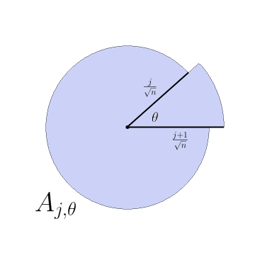
As discussed in Step 3 of the outline, to bound the deviations of λk\lambda_{k} about its predicted location λ~k\tilde{\lambda}_{k}, we first use Proposition 4 to bound the deviations of the counting functions for initial segments with respect to the order ≺\prec. Specifically, we will consider 𝒩⁡(Aj,θ)\mathcal{N}(A_{j,\theta}), where

Aj,θ:={z∈ℂ|z≺jn​ei​θ}={z∈ℂ||z|<jn}∪{z∈ℂ|jn≤|z|<j+1n, 0<argz≤θ},\begin{split}A_{j,\theta}&:=\left\{z\in\mathbb{C}\mathrel{}\middle|\mathrel{}z\prec\frac{j}{\sqrt{n}}e^{i\theta}\right\}\\ &=\left\{z\in\mathbb{C}\mathrel{}\middle|\mathrel{}\left|z\right|<\frac{j}{\sqrt{n}}\right\}\cup\left\{z\in\mathbb{C}\mathrel{}\middle|\mathrel{}\frac{j}{\sqrt{n}}\leq\left|z\right|<\frac{j+1}{\sqrt{n}},\ 0<\arg z\leq\theta\right\},\end{split}

for 1≤j≤n−11\leq j\leq\sqrt{n}-1 and 0<θ≤2​π0<\theta\leq 2\pi (see Figure 1).

Refer to caption
Figure 1.

Finally, we conclude this section by collecting a few known formulas and estimates which will be used repeatedly below. The following integral formula can be proved by repeated integration by parts; we omit the proof.

Lemma 5.

If kk is a nonnegative integer and a>0a>0, then

1k!​∫a∞sk​e−s​𝑑s=e−a​∑ℓ=0kaℓℓ!,\frac{1}{k!}\int_{a}^{\infty}s^{k}e^{-s}\ ds=e^{-a}\sum_{\ell=0}^{k}\frac{a^{\ell}}{\ell!},

and consequently

1k!​∫0ask​e−s​𝑑s=e−a​∑ℓ=k+1∞aℓℓ!.\frac{1}{k!}\int_{0}^{a}s^{k}e^{-s}\ ds=e^{-a}\sum_{\ell=k+1}^{\infty}\frac{a^{\ell}}{\ell!}.

The following inequality follows from a standard Chernoff bound argument for Poisson random variables.

Lemma 6.

If 0<λ≤n0<\lambda\leq n, then ∑k=n∞λkk!≤(e​λn)n.\sum_{k=n}^{\infty}\frac{\lambda^{k}}{k!}\leq\left(\frac{e\lambda}{n}\right)^{n}.

Proof.

Let XX have a Poisson distribution with parameter λ\lambda. Assuming for simplicity that λ<n\lambda<n, let t=log⁡(n/λ)>0t=\log(n/\lambda)>0. Then

∑k=n∞λkk!=eλℙ[X≥n]≤eλ−t​n𝔼et​X=eλ​et−t​n=(e​λn)n.∎\sum_{k=n}^{\infty}\frac{\lambda^{k}}{k!}=e^{\lambda}\mathbb{P}\left[X\geq n\right]\leq e^{\lambda-tn}\mathbb{E}e^{tX}=e^{\lambda e^{t}-tn}=\left(\frac{e\lambda}{n}\right)^{n}.\qed

Finally, we will use the following uniform version of Stirling’s approximation.

Lemma 7.

For each positive integer nn, 2​π​nn+12​e−n≤n!≤e​nn+12​e−n.\sqrt{2\pi}n^{n+\frac{1}{2}}e^{-n}\leq n!\leq en^{n+\frac{1}{2}}e^{-n}.

Proof.

The following version of Stirling’s approximation appears as [5, (9.15)]:

2​π​nn+12​e−n+112​n+1<n!<2​π​nn+12​e−n+112​n.\sqrt{2\pi}n^{n+\frac{1}{2}}e^{-n+\frac{1}{12n+1}}<n!<\sqrt{2\pi}n^{n+\frac{1}{2}}e^{-n+\frac{1}{12n}}.

The lemma is trivially true when n=1n=1, and for n≥2n\geq 2, the lemma follows since 2​π​e1/12​n≤2​π​e1/24<e\sqrt{2\pi}e^{1/12n}\leq\sqrt{2\pi}e^{1/24}<e. ∎

3. Means and variances

Concentration inequalities for the random variables 𝒩⁡(Aj,θ)\mathcal{N}\left(A_{j,\theta}\right) about their means follow from Proposition 4, but in order to make use of them, fairly sharp estimates on the means and variances of the 𝒩⁡(Aj,θ)\mathcal{N}\left(A_{j,\theta}\right) are needed. These estimates, like the proof of Proposition 4, make use of the determinantal point process structure of the eigenvalues of GnG_{n}.

Proposition 8.

If A⊆DA\subseteq D,

n​|A|π−e​n≤𝔼​𝒩​(A)≤n​|A|π,\frac{n\left|A\right|}{\pi}-e\sqrt{n}\leq\mathbb{E}\mathcal{N}(A)\leq\frac{n\left|A\right|}{\pi},

where |A|\left|A\right| denotes the area of AA. Moreover, if A⊆(1−log⁡nn)​DA\subseteq\left(1-\sqrt{\frac{\log n}{n}}\right)D, then

n​|A|π−e2≤𝔼​𝒩​(A)≤n​|A|π.\frac{n\left|A\right|}{\pi}-e^{2}\leq\mathbb{E}\mathcal{N}(A)\leq\frac{n\left|A\right|}{\pi}.
Proof.

The determinantal point process structure of the eigenvalues of GnG_{n} implies that that 𝔼​𝒩​(A)=∫n​AK⁡(z,z)​𝑑z\mathbb{E}\mathcal{N}(A)=\int_{\sqrt{n}A}K(z,z)\ dz (where d​zdz denotes integration with respect to Lebesgue measure on ℂ\mathbb{C}), so that

𝔼​𝒩​(A)=1π​∫n​A(1−∑k=n∞e−|z|2​|z|2​kk!)​𝑑z=n​|A|π−1π​∫n​A∑k=n∞e−|z|2​|z|2​kk!​𝑑z.\mathbb{E}\mathcal{N}(A)=\frac{1}{\pi}\int_{\sqrt{n}A}\left(1-\sum_{k=n}^{\infty}e^{-\left|z\right|^{2}}\frac{\left|z\right|^{2k}}{k!}\right)\ dz=\frac{n\left|A\right|}{\pi}-\frac{1}{\pi}\int_{\sqrt{n}A}\sum_{k=n}^{\infty}e^{-\left|z\right|^{2}}\frac{\left|z\right|^{2k}}{k!}\ dz.

Using Lemma 6 and then integrating in polar coordinates,

1π​∫n​A∑k=n∞e−|z|2​|z|2​kk!​𝑑z\displaystyle\frac{1}{\pi}\int_{\sqrt{n}A}\sum_{k=n}^{\infty}e^{-\left|z\right|^{2}}\frac{\left|z\right|^{2k}}{k!}\ dz ≤(en)n​∫n​De−|z|2​|z|2​n​𝑑z\displaystyle\leq\left(\frac{e}{n}\right)^{n}\int_{\sqrt{n}D}e^{-\left|z\right|^{2}}\left|z\right|^{2n}\ dz
=2​(en)n​∫0ne−r2​r2​n+1​𝑑r<(en)n​n!≤π​e​n,\displaystyle=2\left(\frac{e}{n}\right)^{n}\int_{0}^{\sqrt{n}}e^{-r^{2}}r^{2n+1}\ dr<\left(\frac{e}{n}\right)^{n}n!\leq\pi e\sqrt{n},

by Stirling’s approximation (Lemma 7).

If A⊆r​DA\subseteq rD for r≤1r\leq 1 then, using Lemmas 6, 5, and 6 again,

1π​∫n​r​D∑k=n∞e−|z|2​|z|2​kk!​𝑑z≤(en)n​∫0r2​ne−s​sn​𝑑s=e−r2​n​(en)n​n!​∑ℓ=n+1∞(r2​n)ℓℓ!≤e−r2​nen(er2)n≤e2ne−n(1−r2)2/2,\begin{split}\frac{1}{\pi}\int_{\sqrt{n}rD}\sum_{k=n}^{\infty}e^{-\left|z\right|^{2}}\frac{\left|z\right|^{2k}}{k!}\ dz&\leq\left(\frac{e}{n}\right)^{n}\int_{0}^{r^{2}n}e^{-s}s^{n}\ ds\\ &=e^{-r^{2}n}\left(\frac{e}{n}\right)^{n}n!\sum_{\ell=n+1}^{\infty}\frac{(r^{2}n)^{\ell}}{\ell!}\\ &\leq e^{-r^{2}n}e\sqrt{n}(er^{2})^{n}\leq e^{2}\sqrt{n}e^{-n(1-r^{2})^{2}/2},\end{split}

since log⁡(1−ε)≤−ε−ε2/2\log(1-\varepsilon)\leq-\varepsilon-\varepsilon^{2}/2 for 0<ε<10<\varepsilon<1. Finally, let r=1−log⁡nnr=1-\sqrt{\frac{\log n}{n}}. Then ne−n(1−r2)2/2≤ne−n(1−r)2/2=1.\sqrt{n}e^{-n(1-r^{2})^{2}/2}\leq\sqrt{n}e^{-n(1-r)^{2}/2}=1. ∎

We will also need estimates for the expected number of eigenvalues outside of discs of radius R≥1R\geq 1.

Proposition 9.

For each R≥1R\geq 1, 𝔼​𝒩​(ℂ∖R​D)≤12​π​n​en​R2​(n−1)​e−n​R2.\mathbb{E}\mathcal{N}(\mathbb{C}\setminus RD)\leq\frac{1}{\sqrt{2\pi}}\sqrt{n}e^{n}R^{2(n-1)}e^{-nR^{2}}.

Proof.

Again using the determinantal point process kernel in (2),

𝔼​𝒩​(ℂ∖R​D)\displaystyle\mathbb{E}\mathcal{N}(\mathbb{C}\setminus RD) =1π​∑k=0n−11k!​∫ℂ∖n​R​De−|z|2​|z|2​k​𝑑z\displaystyle=\frac{1}{\pi}\sum_{k=0}^{n-1}\frac{1}{k!}\int_{\mathbb{C}\setminus\sqrt{n}RD}e^{-\left|z\right|^{2}}\left|z\right|^{2k}\ dz
=∑k=0n−11k!​∫n​R2∞rk​e−r​𝑑r\displaystyle=\sum_{k=0}^{n-1}\frac{1}{k!}\int_{nR^{2}}^{\infty}r^{k}e^{-r}\ dr
=e−n​R2​∑k=0n−1∑ℓ=0k(n​R2)ℓℓ!\displaystyle=e^{-nR^{2}}\sum_{k=0}^{n-1}\sum_{\ell=0}^{k}\frac{(nR^{2})^{\ell}}{\ell!}
=e−n​R2​∑ℓ=0n−1(n​R2)ℓℓ!​(n−ℓ)\displaystyle=e^{-nR^{2}}\sum_{\ell=0}^{n-1}\frac{(nR^{2})^{\ell}}{\ell!}(n-\ell)
=n​e−n​R2​(∑ℓ=0n−1(n​R2)ℓℓ!−R2​∑ℓ=0n−2(n​R2)ℓℓ!)\displaystyle=ne^{-nR^{2}}\left(\sum_{\ell=0}^{n-1}\frac{(nR^{2})^{\ell}}{\ell!}-R^{2}\sum_{\ell=0}^{n-2}\frac{(nR^{2})^{\ell}}{\ell!}\right)
=n​e−n​R2​((n​R2)n−1(n−1)!−(R2−1)​∑ℓ=0n−2(n​R2)ℓℓ!)\displaystyle=ne^{-nR^{2}}\left(\frac{(nR^{2})^{n-1}}{(n-1)!}-(R^{2}-1)\sum_{\ell=0}^{n-2}\frac{(nR^{2})^{\ell}}{\ell!}\right)
≤n​e−n​R2​(n​R2)n−1(n−1)!\displaystyle\leq ne^{-nR^{2}}\frac{(nR^{2})^{n-1}}{(n-1)!}
≤12​π​e−n​R2​n​en​R2​(n−1)\displaystyle\leq\frac{1}{\sqrt{2\pi}}e^{-nR^{2}}\sqrt{n}e^{n}R^{2(n-1)}

by Stirling’s approximation. ∎

Proposition 10.

For each 1≤j≤n−11\leq j\leq\sqrt{n}-1 and 0≤θ≤2​π0\leq\theta\leq 2\pi,

Var⁡𝒩⁡(Aj,θ)≤16​j.\var\mathcal{N}(A_{j,\theta})\leq 16j.

The constant 1616 in the statement of Proposition 10 is not optimal and is included only for the sake of concreteness.

Proof.

By an argument in [8, Appendix B],

(3) Var⁡(𝒩⁡(Aj,θ))=∫{|z|≤j}∫{|w|≥j+1}|K(z,w)|2dwdz+∫{|z|≤j}∫{j≤|w|≤j+1,argw≥θ}|K(z,w)|2dwdz+∫{j≤|z|≤j+1,argz≤θ}∫{|w|≥j+1}|K(z,w)|2dwdz+∫{j≤|z|≤j+1,argz≤θ}∫{j≤|w|≤j+1,argw≥θ}|K(z,w)|2dwdz\begin{split}\var(\mathcal{N}(A_{j,\theta}))&=\int\limits_{\{\left|z\right|\leq j\}}\int\limits_{\{\left|w\right|\geq j+1\}}\left|K(z,w)\right|^{2}\ dw\ dz\\ &\quad+\int\limits_{\{\left|z\right|\leq j\}}\int\limits_{\{j\leq\left|w\right|\leq j+1,\ \arg w\geq\theta\}}\left|K(z,w)\right|^{2}\ dw\ dz\\ &\quad+\int\limits_{\{j\leq\left|z\right|\leq j+1,\ \arg z\leq\theta\}}\int\limits_{\{\left|w\right|\geq j+1\}}\left|K(z,w)\right|^{2}\ dw\ dz\\ &\quad+\int\limits_{\{j\leq\left|z\right|\leq j+1,\ \arg z\leq\theta\}}\int\limits_{\{j\leq\left|w\right|\leq j+1,\ \arg w\geq\theta\}}\left|K(z,w)\right|^{2}\ dw\ dz\end{split}

Observe that

|K⁡(r1​ei​φ1,r2​ei​φ2)|2=1π2​∑k,ℓ=0n−11k!​ℓ!​e−(r12+r22)​(r1​r2)k+ℓ​ei⁡(k−ℓ)​(φ1−φ2).\left|K(r_{1}e^{i\varphi_{1}},r_{2}e^{i\varphi_{2}})\right|^{2}=\frac{1}{\pi^{2}}\sum_{k,\ell=0}^{n-1}\frac{1}{k!\ell!}e^{-(r_{1}^{2}+r_{2}^{2})}(r_{1}r_{2})^{k+\ell}e^{i(k-\ell)(\varphi_{1}-\varphi_{2})}.

Integrating in polar coordinates, the first integral in (3) is

1π2\displaystyle\frac{1}{\pi^{2}} ∑k,ℓ=0n−11k!​ℓ!​∫0jrk+ℓ+1​e−r2​𝑑r​∫j+1∞rk+ℓ+1​e−r2​𝑑r​∫02​πei​φ​(k−ℓ)​𝑑φ​∫02​πei​φ​(ℓ−k)​𝑑φ\displaystyle\sum_{k,\ell=0}^{n-1}\frac{1}{k!\ell!}\int_{0}^{j}r^{k+\ell+1}e^{-r^{2}}\ dr\int_{j+1}^{\infty}r^{k+\ell+1}e^{-r^{2}}\ dr\int_{0}^{2\pi}e^{i\varphi(k-\ell)}\ d\varphi\int_{0}^{2\pi}e^{i\varphi(\ell-k)}\ d\varphi
=∑k=0n−11k!2​∫0j2sk​e−s​𝑑s​∫(j+1)2∞sk​e−s​𝑑s\displaystyle=\sum_{k=0}^{n-1}\frac{1}{k!^{2}}\int_{0}^{j^{2}}s^{k}e^{-s}\ ds\int_{(j+1)^{2}}^{\infty}s^{k}e^{-s}\ ds
≤∑k=0j21k!​∫j2∞sk​e−s​𝑑s+∑k=(j+1)2n−11k!​∫0(j+1)2sk​e−s​𝑑s+(2​j+1).\displaystyle\leq\sum_{k=0}^{j^{2}}\frac{1}{k!}\int_{j^{2}}^{\infty}s^{k}e^{-s}\ ds+\sum_{k=(j+1)^{2}}^{n-1}\frac{1}{k!}\int_{0}^{(j+1)^{2}}s^{k}e^{-s}\ ds+(2j+1).

Here we have used that the angular integrals are nonzero only if k=ℓk=\ell, and that the integrals in the second line are bounded by k!k!. Note also that if j2<n−1<(j+1)2j^{2}<n-1<(j+1)^{2}, the second term is not needed, and if j2≥n−1j^{2}\geq n-1, then the second and third terms are not needed. By Lemma 5 and Stirling’s approximation,

∑k=0j21k!​∫j2∞sk​e−s​𝑑s=∑k=0j2e−j2​∑ℓ=0kj2​ℓℓ!=e−j2​∑ℓ=0j2∑k=ℓj2j2​ℓℓ!=e−j2​∑ℓ=0j2j2​ℓℓ!​(j2−ℓ+1)≤1+e−j2​(∑ℓ=0j2j2​(ℓ+1)ℓ!−∑ℓ=1j2j2​ℓ(ℓ−1)!)=1+e−j2​j2​(j2+1)(j2)!≤1+j2​π,\begin{split}\sum_{k=0}^{j^{2}}\frac{1}{k!}\int_{j^{2}}^{\infty}s^{k}e^{-s}ds&=\sum_{k=0}^{j^{2}}e^{-j^{2}}\sum_{\ell=0}^{k}\frac{j^{2\ell}}{\ell!}=e^{-j^{2}}\sum_{\ell=0}^{j^{2}}\sum_{k=\ell}^{j^{2}}\frac{j^{2\ell}}{\ell!}=e^{-j^{2}}\sum_{\ell=0}^{j^{2}}\frac{j^{2\ell}}{\ell!}(j^{2}-\ell+1)\\ &\leq 1+e^{-j^{2}}\left(\sum_{\ell=0}^{j^{2}}\frac{j^{2(\ell+1)}}{\ell!}-\sum_{\ell=1}^{j^{2}}\frac{j^{2\ell}}{(\ell-1)!}\right)\\ &=1+e^{-j^{2}}\frac{j^{2(j^{2}+1)}}{(j^{2})!}\leq 1+\frac{j}{\sqrt{2\pi}},\end{split}

and

∑k=(j+1)2n−11k!​∫0(j+1)2sk​e−s​𝑑s=e−(j+1)2​∑k=(j+1)2n−1∑ℓ=k+1∞(j+1)2​ℓℓ!=e−(j+1)2​∑ℓ=(j+1)2+1∞(j+1)2​ℓℓ!​(ℓ−(j+1)2)=e−(j+1)2​(∑ℓ=(j+1)2+1∞(j+1)2​ℓ(ℓ−1)!−∑ℓ=(j+1)2+1∞(j+1)2​(ℓ+1)ℓ!)=e−(j+1)2​(j+1)2​((j+1)2+1)(j+1)2!≤j+12​π.\begin{split}\sum_{k=(j+1)^{2}}^{n-1}\frac{1}{k!}\int_{0}^{(j+1)^{2}}s^{k}e^{-s}\ ds&=e^{-(j+1)^{2}}\sum_{k=(j+1)^{2}}^{n-1}\sum_{\ell=k+1}^{\infty}\frac{(j+1)^{2\ell}}{\ell!}\\ &=e^{-(j+1)^{2}}\sum_{\ell=(j+1)^{2}+1}^{\infty}\frac{(j+1)^{2\ell}}{\ell!}\left(\ell-(j+1)^{2}\right)\\ &=e^{-(j+1)^{2}}\left(\sum_{\ell=(j+1)^{2}+1}^{\infty}\frac{(j+1)^{2\ell}}{(\ell-1)!}-\sum_{\ell=(j+1)^{2}+1}^{\infty}\frac{(j+1)^{2(\ell+1)}}{\ell!}\right)\\ &=e^{-(j+1)^{2}}\frac{(j+1)^{2((j+1)^{2}+1)}}{(j+1)^{2}!}\leq\frac{j+1}{\sqrt{2\pi}}.\end{split}

The second integral in (3) is equal to

1π2∑k,ℓ=0n−11k!​ℓ!​∫0jrk+ℓ+1​e−r2​𝑑r​∫jj+1rk+ℓ+1​e−r2​𝑑r​∫02​πei​φ​(k−ℓ)​𝑑φ​∫θ2​πei​φ​(ℓ−k)​𝑑φ=(1−θ2​π)​∑k=0n−1(1k!​∫0j2sk​e−s​ds)​(1k!​∫j2(j+1)2sk​e−s​ds)≤(1−θ2​π)​∑k=0n−11k!​∫j2(j+1)2sk​e−s​𝑑s\begin{split}\frac{1}{\pi^{2}}&\sum_{k,\ell=0}^{n-1}\frac{1}{k!\ell!}\int_{0}^{j}r^{k+\ell+1}e^{-r^{2}}\ dr\int_{j}^{j+1}r^{k+\ell+1}e^{-r^{2}}\ dr\int_{0}^{2\pi}e^{i\varphi(k-\ell)}\ d\varphi\int_{\theta}^{2\pi}e^{i\varphi(\ell-k)}\ d\varphi\\ &=\left(1-\frac{\theta}{2\pi}\right)\sum_{k=0}^{n-1}\left(\frac{1}{k!}\int_{0}^{j^{2}}s^{k}e^{-s}\ ds\right)\left(\frac{1}{k!}\int_{j^{2}}^{(j+1)^{2}}s^{k}e^{-s}\ ds\right)\\ &\leq\left(1-\frac{\theta}{2\pi}\right)\sum_{k=0}^{n-1}\frac{1}{k!}\int_{j^{2}}^{(j+1)^{2}}s^{k}e^{-s}\ ds\end{split}

since the first angular integral is nonzero only for k=ℓk=\ell, and the third integral in (3) is similarly bounded by

θ2​π​∑k=0n−11k!​∫j2(j+1)2sk​e−s​𝑑s.\frac{\theta}{2\pi}\sum_{k=0}^{n-1}\frac{1}{k!}\int_{j^{2}}^{(j+1)^{2}}s^{k}e^{-s}\ ds.

The function s↦sk​e−ss\mapsto s^{k}e^{-s} is unimodal for s>0s>0 and takes on its maximum value at s=ks=k, so

∫j2(j+1)2ske−sds≤{(2​j+1)​j2​k​e−j2when ​k≤j2,(2​j+1)​(j+1)2​k​e−(j+1)2when k≥(j+1)2, andk!always.\int_{j^{2}}^{(j+1)^{2}}s^{k}e^{-s}\ ds\leq\begin{cases}(2j+1)j^{2k}e^{-j^{2}}&\text{when }k\leq j^{2},\\ (2j+1)(j+1)^{2k}e^{-(j+1)^{2}}&\text{when }k\geq(j+1)^{2},\text{ and}\\ k!&\text{always.}\end{cases}

From this it follows that the sum of the second and third integrals in (3) is bounded by

(4) ∑k=0n−11k!​∫j2(j+1)2sk​e−s​𝑑s≤3​(2​j+1).\sum_{k=0}^{n-1}\frac{1}{k!}\int_{j^{2}}^{(j+1)^{2}}s^{k}e^{-s}\ ds\leq 3(2j+1).

The final integral in (3) is equal to

(5) 1π2∑k,ℓ=0n−11k!​ℓ!​(∫jj+1rk+ℓ+1​e−r2​dr)2​∫0θei​φ​(k−ℓ)​dφ​∫θ2​πei​φ​(ℓ−k)​dφ.\begin{split}\frac{1}{\pi^{2}}&\sum_{k,\ell=0}^{n-1}\frac{1}{k!\ell!}\left(\int_{j}^{j+1}r^{k+\ell+1}e^{-r^{2}}\ dr\right)^{2}\int_{0}^{\theta}e^{i\varphi(k-\ell)}\ d\varphi\int_{\theta}^{2\pi}e^{i\varphi(\ell-k)}\ d\varphi.\end{split}

For k≠ℓk\neq\ell,

∫θ2​πei​φ​(ℓ−k)​𝑑φ=−∫0θei​φ​(ℓ−k)dφ=−∫0θei​φ​(k−ℓ)​dφ¯\begin{split}\int_{\theta}^{2\pi}e^{i\varphi(\ell-k)}\ d\varphi&=-\int_{0}^{\theta}e^{i\varphi(\ell-k)}\ d\varphi=-\overline{\int_{0}^{\theta}e^{i\varphi(k-\ell)}\ d\varphi}\end{split}

so each summand in (5) with k≠ℓk\neq\ell is negative. Thus (5) is bounded by

θ⁡(2​π−θ)π2​∑k=0n−1(1k!​∫jj+1r2​k+1​e−r2​𝑑r)2=θ2​π​(1−θ2​π)​∑k=0n−1(1k!​∫j2(j+1)2sk​e−s​𝑑s)2,\frac{\theta(2\pi-\theta)}{\pi^{2}}\sum_{k=0}^{n-1}\left(\frac{1}{k!}\int_{j}^{j+1}r^{2k+1}e^{-r^{2}}\ dr\right)^{2}=\frac{\theta}{2\pi}\left(1-\frac{\theta}{2\pi}\right)\sum_{k=0}^{n-1}\left(\frac{1}{k!}\int_{j^{2}}^{(j+1)^{2}}s^{k}e^{-s}\ ds\right)^{2},

which by (4) is less than 34​(2​j+1)\frac{3}{4}(2j+1). ∎

4. Deviations

The goal of this section is to obtain sharp concentration results for the eigenvalues λk\lambda_{k} about their predicted locations λ~k\tilde{\lambda}_{k}. Recall that we only defined λ~k\tilde{\lambda}_{k} for a restricted range of kk; for the outermost eigenvalues, for which we did not define λ~k\tilde{\lambda}_{k}, we will make use of the following sloppy estimate.

Lemma 11.

For each kk and any random variable α∈ℂ\alpha\in\mathbb{C} with |α|≤1\left|\alpha\right|\leq 1,

𝔼​|λk−α|p≤4p+(43)p−1​(2n)p2​Γ​(1+p2).\mathbb{E}\left|\lambda_{k}-\alpha\right|^{p}\leq 4^{p}+\left(\frac{4}{3}\right)^{p-1}\left(\frac{2}{n}\right)^{\frac{p}{2}}\Gamma\left(1+\frac{p}{2}\right).

and

ℙ[|λk−α|≥t]≤e−nt2/4\mathbb{P}\left[\left|\lambda_{k}-\alpha\right|\geq t\right]\leq e^{-nt^{2}/4}

for t>4t>4.

Proof.

For any t≥1t\geq 1,

(6) ℙ[|λk−α|≥t]≤ℙ[|λk|≥t−1]≤ℙ[𝒩(ℂ∖(t−1)D)≥1]≤𝔼𝒩(ℂ∖(t−1)D),\mathbb{P}\left[\left|\lambda_{k}-\alpha\right|\geq t\right]\leq\mathbb{P}\left[\left|\lambda_{k}\right|\geq t-1\right]\leq\mathbb{P}\left[\mathcal{N}(\mathbb{C}\setminus(t-1)D)\geq 1\right]\leq\mathbb{E}\mathcal{N}(\mathbb{C}\setminus(t-1)D),

by Markov’s inequality. Proposition 9 implies that for any R>1R>1,

𝔼​𝒩​(ℂ∖R​D)≤exp⁡[−(R2−32−2​log⁡R)​n],\mathbb{E}\mathcal{N}(\mathbb{C}\setminus RD)\leq\exp\left[-\left(R^{2}-\frac{3}{2}-2\log R\right)n\right],

since log⁡n≤n\log n\leq n. For R>3R>3,

R2−32−2​log⁡R>R22,R^{2}-\frac{3}{2}-2\log R>\frac{R^{2}}{2},

and so

(7) 𝔼𝒩(ℂ∖RD)≤e−nR2/2.\mathbb{E}\mathcal{N}(\mathbb{C}\setminus RD)\leq e^{-nR^{2}/2}.

Combining (6) and (7), we obtain

𝔼​|λk−α|p=∫0∞ptp−1ℙ[|λk−α|≥t]dt≤∫04ptp−1dt+∫4∞ptp−1e−n(t−1)2/2dt≤4p+(43)p−1p∫3∞sp−1e−ns2/2ds≤4p+(43)p−1​(2n)p2​Γ​(1+p2)∎\begin{split}\mathbb{E}\left|\lambda_{k}-\alpha\right|^{p}&=\int_{0}^{\infty}pt^{p-1}\mathbb{P}\left[\left|\lambda_{k}-\alpha\right|\geq t\right]\ dt\\ &\leq\int_{0}^{4}pt^{p-1}\ dt+\int_{4}^{\infty}pt^{p-1}e^{-n(t-1)^{2}/2}\ dt\\ &\leq 4^{p}+\left(\frac{4}{3}\right)^{p-1}p\int_{3}^{\infty}s^{p-1}e^{-ns^{2}/2}\ ds\\ &\leq 4^{p}+\left(\frac{4}{3}\right)^{p-1}\left(\frac{2}{n}\right)^{\frac{p}{2}}\Gamma\left(1+\frac{p}{2}\right)\qed\end{split}

and

ℙ[|λk−α|≥t]≤e−n(t−1)2/2≤e−nt2/4\mathbb{P}\left[\left|\lambda_{k}-\alpha\right|\geq t\right]\leq e^{-n(t-1)^{2}/2}\leq e^{-nt^{2}/4}

for t>4t>4.

We will need stronger concentration for most of the eigenvalues, which we get as a consequence of the following.

Proposition 12.

For each 1≤j≤n−1−11\leq j\leq\sqrt{n-1}-1, 0≤θ≤2​π0\leq\theta\leq 2\pi, and t>0t>0,

ℙ[𝒩(Aj,θ)−n​|Aj,θ|π≥t]≤exp[−min{t264​j,t2}].\mathbb{P}\left[\mathcal{N}(A_{j,\theta})-\frac{n\left|A_{j,\theta}\right|}{\pi}\geq t\right]\leq\exp\left[-\min\left\{\frac{t^{2}}{64j},\frac{t}{2}\right\}\right].

If j≤n−log⁡n−1j\leq\sqrt{n}-\sqrt{\log n}-1, then

ℙ[n​|Aj,θ|π−𝒩(Aj,θ)≥t]≤3exp[−min{t2256​j,t4}].\mathbb{P}\left[\frac{n\left|A_{j,\theta}\right|}{\pi}-\mathcal{N}(A_{j,\theta})\geq t\right]\leq 3\exp\left[-\min\left\{\frac{t^{2}}{256j},\frac{t}{4}\right\}\right].
Proof.

The first claim follows immediately from Propositions 4, 8, and 10. For the second, the assumption on jj implies that Aj,θ⊆(1−log⁡nn)​DA_{j,\theta}\subseteq\left(1-\sqrt{\frac{\log n}{n}}\right)D, and so by Propositions 4, 8, and 10,

ℙ[n​|Aj,θ|π−𝒩(Aj,θ)≥t]≤ℙ[𝔼𝒩(Aj,θ)−𝒩(Aj,θ)≥t−e2]≤exp⁡[−min⁡{(t−e2)264​j,t−e22}]\begin{split}\mathbb{P}\left[\frac{n\left|A_{j,\theta}\right|}{\pi}-\mathcal{N}(A_{j,\theta})\geq t\right]&\leq\mathbb{P}\left[\mathbb{E}\mathcal{N}(A_{j,\theta})-\mathcal{N}(A_{j,\theta})\geq t-e^{2}\right]\\ &\leq\exp\left[-\min\left\{\frac{(t-e^{2})^{2}}{64j},\frac{t-e^{2}}{2}\right\}\right]\end{split}

for t>e2t>e^{2}. If t≥2​e2t\geq 2e^{2}, then t−e2≥t/2t-e^{2}\geq t/2, so

ℙ[𝔼𝒩(Aj,θ)−𝒩(Aj,θ)≥t]≤exp[−min{t2256​j,t4}].\mathbb{P}\left[\mathbb{E}\mathcal{N}(A_{j,\theta})-\mathcal{N}(A_{j,\theta})\geq t\right]\leq\exp\left[-\min\left\{\frac{t^{2}}{256j},\frac{t}{4}\right\}\right].

On the other hand, if t<2​e2t<2e^{2}, then

exp[−min{t2256​j,t4}]>e−e4/64>1/3,\exp\left[-\min\left\{\frac{t^{2}}{256j},\frac{t}{4}\right\}\right]>e^{-e^{4}/64}>1/3,

which implies the second claim. ∎

The concentration inequalities for the 𝒩⁡(Aj,θ)\mathcal{N}(A_{j,\theta}) together with geometric arguments yield the following concentration for individual eigenvalues.

Theorem 13.

There are constants C,c>0C,c>0 such that for those kk with ℓ=⌈k⌉≤n−log⁡n\ell=\lceil\sqrt{k}\rceil\leq\sqrt{n}-\sqrt{\log n},

  • —

    when 9≤s≤π⁡(ℓ−1)+29\leq s\leq\pi(\ell-1)+2,

    ℙ[|λk−λ~k|>sn]≤Cexp[−min{(s−9)2256​π2​(ℓ−1),s−94​π}];\mathbb{P}\left[\left|\lambda_{k}-\tilde{\lambda}_{k}\right|>\frac{s}{\sqrt{n}}\right]\leq C\exp\left[-\min\left\{\frac{(s-9)^{2}}{256\pi^{2}(\ell-1)},\frac{s-9}{4\pi}\right\}\right];
  • —

    when s>π⁡(ℓ−1)+2,s>\pi(\ell-1)+2,

    ℙ[|λk−λ~k|>sn]≤Ce−c​s2.\mathbb{P}\left[\left|\lambda_{k}-\tilde{\lambda}_{k}\right|>\frac{s}{\sqrt{n}}\right]\leq Ce^{-cs^{2}}.
Proof.

Trivially,

ℙ[|λk−λ~k|≥t]=ℙ[|λk−λ~k|≥t and λk≺λ~k]+ℙ[|λk−λ~k|≥t and λk≻λ~k].\mathbb{P}\left[\left|\lambda_{k}-\tilde{\lambda}_{k}\right|\geq t\right]=\mathbb{P}\left[\left|\lambda_{k}-\tilde{\lambda}_{k}\right|\geq t\text{ and }\lambda_{k}\prec\tilde{\lambda}_{k}\right]+\mathbb{P}\left[\left|\lambda_{k}-\tilde{\lambda}_{k}\right|\geq t\text{ and }\lambda_{k}\succ\tilde{\lambda}_{k}\right].

Case 1: λk≺λ~k\lambda_{k}\prec\tilde{\lambda}_{k}.

With probability 11, λk≺λ~k\lambda_{k}\prec\tilde{\lambda}_{k} implies that either

ℓ−1n≤|λk|<ℓna​n​darg⁡λk<arg⁡λ~k=2​π​q2​ℓ−1.\frac{\ell-1}{\sqrt{n}}\leq\left|\lambda_{k}\right|<\frac{\ell}{\sqrt{n}}\qquad and\qquad\arg\lambda_{k}<\arg\tilde{\lambda}_{k}=\frac{2\pi q}{2\ell-1}.

or

|λk|<|λ~k|=ℓ−1n.\left|\lambda_{k}\right|<\left|\tilde{\lambda}_{k}\right|=\frac{\ell-1}{\sqrt{n}}.

Observe that, in either case, |λk−λ~k|<2​ℓ−1n\left|\lambda_{k}-\tilde{\lambda}_{k}\right|<\frac{2\ell-1}{\sqrt{n}}.

If |λk−λ~k|≥s/n\left|\lambda_{k}-\tilde{\lambda}_{k}\right|\geq s/\sqrt{n} and a⁡(θ,φ)a(\theta,\varphi) denotes the length of the shorter arc on the unit circle between ei​θe^{i\theta} and ei​φe^{i\varphi}, then the elementary estimate

|R​ei​θ−r​ei​φ|≤r⋅a⁡(θ,φ)+|R−r|,\left|Re^{i\theta}-re^{i\varphi}\right|\leq r\cdot a(\theta,\varphi)+\left|R-r\right|,

implies that when |λk|∈[ℓ−2n,ℓn)\left|\lambda_{k}\right|\in\left[\frac{\ell-2}{\sqrt{n}},\frac{\ell}{\sqrt{n}}\right) and s≥1s\geq 1,

(8) a⁡(arg⁡λk,2​π​q2​ℓ−1)≥s−1ℓ−1.a\left(\arg\lambda_{k},\frac{2\pi q}{2\ell-1}\right)\geq\frac{s-1}{\ell-1}.

Suppose that s−1ℓ−1<2​π​q2​ℓ−1\frac{s-1}{\ell-1}<\frac{2\pi q}{2\ell-1}. Since either |λk|<ℓ−1n\left|\lambda_{k}\right|<\frac{\ell-1}{\sqrt{n}} or arg⁡λk<2​π​q2​ℓ−1\arg{\lambda_{k}}<\frac{2\pi q}{2\ell-1}, Inequality (8) implies that

λk≺ℓ−1n​exp⁡[i⁡(2​π​q2​ℓ−1−s−1ℓ−1)],\lambda_{k}\prec\frac{\ell-1}{\sqrt{n}}\exp\left[i\left(\frac{2\pi q}{2\ell-1}-\frac{s-1}{\ell-1}\right)\right],

and so

𝒩⁡(Aℓ−1,2​π​q2​ℓ−1−s−1ℓ−1)≥k=(ℓ−1)2+q.\mathcal{N}\bigl(A_{\ell-1,\frac{2\pi q}{2\ell-1}-\frac{s-1}{\ell-1}}\bigr)\geq k=(\ell-1)^{2}+q.

Since

nπ​|Aj,θ|=j2+θ2​π​(2​j+1),\frac{n}{\pi}\left|A_{j,\theta}\right|=j^{2}+\frac{\theta}{2\pi}(2j+1),

we have

nπ​|Aℓ−1,2​π​q2​ℓ−1−s−1ℓ−1|=k−2​ℓ−12​π​(ℓ−1)​(s−1)≤k−s−1π,\frac{n}{\pi}\left|A_{\ell-1,\frac{2\pi q}{2\ell-1}-\frac{s-1}{\ell-1}}\right|=k-\frac{2\ell-1}{2\pi(\ell-1)}(s-1)\leq k-\frac{s-1}{\pi},

and so Proposition 12 implies that

ℙ[𝒩(Aℓ−1,2​π​q2​ℓ−1−s−1ℓ−1)≥k]≤ℙ[𝒩(Aℓ−1,2​π​q2​ℓ−1−s−1ℓ−1)−nπ|Aℓ−1,2​π​q2​ℓ−1−s−1ℓ−1|≥s−1π]≤exp⁡[−min⁡{(s−1)264​π2​(ℓ−1),s−12​π}].\begin{split}\mathbb{P}\left[\mathcal{N}\bigl(A_{\ell-1,\frac{2\pi q}{2\ell-1}-\frac{s-1}{\ell-1}}\bigr)\geq k\right]&\leq\mathbb{P}\left[\mathcal{N}\bigl(A_{\ell-1,\frac{2\pi q}{2\ell-1}-\frac{s-1}{\ell-1}}\bigr)-\frac{n}{\pi}\left|A_{\ell-1,\frac{2\pi q}{2\ell-1}-\frac{s-1}{\ell-1}}\right|\geq\frac{s-1}{\pi}\right]\\ &\leq\exp\left[-\min\left\{\frac{(s-1)^{2}}{64\pi^{2}(\ell-1)},\frac{s-1}{2\pi}\right\}\right].\end{split}

Now suppose that 2​π​q2​ℓ−1≤s−1ℓ−1≤π\frac{2\pi q}{2\ell-1}\leq\frac{s-1}{\ell-1}\leq\pi (note that s−1ℓ−1\frac{s-1}{\ell-1} is a lower bound for the length of a shortest path on the circle, hence the upper bound of π\pi, and that the interval in question is non-empty only if q≤2​ℓ−12q\leq\frac{2\ell-1}{2}). Then

λk≺ℓ−2n​exp⁡[i⁡(2​π+2​π​q2​ℓ−1−s−1ℓ−1)],\lambda_{k}\prec\frac{\ell-2}{\sqrt{n}}\exp\left[i\left(2\pi+\frac{2\pi q}{2\ell-1}-\frac{s-1}{\ell-1}\right)\right],

and so

𝒩⁡(Aℓ−2,2​π+2​π​q2​ℓ−1−s−1ℓ−1)≥k.\mathcal{N}\bigl(A_{\ell-2,2\pi+\frac{2\pi q}{2\ell-1}-\frac{s-1}{\ell-1}}\bigr)\geq k.

Now

nπ​|Aℓ−2,2​π+2​π​q2​ℓ−1−s−1ℓ−1|≤k−2​ℓ−32​π​(ℓ−1)​(s−1)≤k−s−12​π\frac{n}{\pi}\left|A_{\ell-2,2\pi+\frac{2\pi q}{2\ell-1}-\frac{s-1}{\ell-1}}\right|\leq k-\frac{2\ell-3}{2\pi(\ell-1)}(s-1)\leq k-\frac{s-1}{2\pi}

for ℓ≥2\ell\geq 2. Thus in this range of ss Proposition 12 implies that

ℙ[𝒩(Aℓ−2,2​π−2​π​q2​ℓ−1−s−1ℓ−1)≥k]≤ℙ[𝒩(Aℓ−2,2​π−2​π​q2​ℓ−1−s−1ℓ−1)−nπ|Aℓ−2,2​π−2​π​q2​ℓ−1−s−1ℓ−1|≥s−12​π]≤exp⁡[−min⁡{(s−1)2256​π2​(ℓ−1),s−14​π}].\begin{split}\mathbb{P}\left[\mathcal{N}\bigl(A_{\ell-2,2\pi-\frac{2\pi q}{2\ell-1}-\frac{s-1}{\ell-1}}\bigr)\geq k\right]&\leq\mathbb{P}\left[\mathcal{N}\bigl(A_{\ell-2,2\pi-\frac{2\pi q}{2\ell-1}-\frac{s-1}{\ell-1}}\bigr)-\frac{n}{\pi}\left|A_{\ell-2,2\pi-\frac{2\pi q}{2\ell-1}-\frac{s-1}{\ell-1}}\right|\geq\frac{s-1}{2\pi}\right]\\ &\leq\exp\left[-\min\left\{\frac{(s-1)^{2}}{256\pi^{2}(\ell-1)},\frac{s-1}{4\pi}\right\}\right].\end{split}

As observed above, the estimates above cover the entire possible range of ss, and so

ℙ[|λk−λ~k|≥sn and λk≺λ~k]≤exp[−min{(s−1)2256​π2​(ℓ−1),s−14​π}]\mathbb{P}\left[\left|\lambda_{k}-\tilde{\lambda}_{k}\right|\geq\frac{s}{\sqrt{n}}\text{ and }\lambda_{k}\prec\tilde{\lambda}_{k}\right]\leq\exp\left[-\min\left\{\frac{(s-1)^{2}}{256\pi^{2}(\ell-1)},\frac{s-1}{4\pi}\right\}\right]

for all s≥1s\geq 1.

Case 2: λk≻λ~k\lambda_{k}\succ\tilde{\lambda}_{k}.

With probability 11, λk≻λ~k\lambda_{k}\succ\tilde{\lambda}_{k} implies that either

ℓ−1n≤|λk|​<ℓnandarg⁡λk>​arg⁡λ~k=2​π​q2​ℓ−1.\frac{\ell-1}{\sqrt{n}}\leq\left|\lambda_{k}\right|<\frac{\ell}{\sqrt{n}}\quad\text{and}\quad\arg\lambda_{k}>\arg\tilde{\lambda}_{k}=\frac{2\pi q}{2\ell-1}.

or

|λk|≥ℓn.\left|\lambda_{k}\right|\geq\frac{\ell}{\sqrt{n}}.

Observe that if |λk−λ~k|≥s/n\left|\lambda_{k}-\tilde{\lambda}_{k}\right|\geq s/\sqrt{n} and |λk|∈[ℓ−1n,ℓ+1n)\left|\lambda_{k}\right|\in\left[\frac{\ell-1}{\sqrt{n}},\frac{\ell+1}{\sqrt{n}}\right), then as above,

(9) a⁡(arg⁡λk,2​π​q2​ℓ−1)≥s−2ℓ−1a\left(\arg\lambda_{k},\frac{2\pi q}{2\ell-1}\right)\geq\frac{s-2}{\ell-1}

for s≥2s\geq 2. We will need to make different arguments depending on the value of s−2ℓ−1\frac{s-2}{\ell-1}.

  1. (1)

    Suppose first that s−2ℓ−1<2​π−2​π​q2​ℓ−1\frac{s-2}{\ell-1}<2\pi-\frac{2\pi q}{2\ell-1}.

    Since either |λk|≥ℓn\left|\lambda_{k}\right|\geq\frac{\ell}{\sqrt{n}} or arg⁡λk>2​π​q2​ℓ−1\arg\lambda_{k}>\frac{2\pi q}{2\ell-1}, Inequality (9) implies that

    λk≻ℓ−1n​exp⁡[i⁡(2​π​q2​ℓ−1+s−2ℓ−1)],\lambda_{k}\succ\frac{\ell-1}{\sqrt{n}}\exp\left[i\left(\frac{2\pi q}{2\ell-1}+\frac{s-2}{\ell-1}\right)\right],

    and so

    𝒩⁡(Aℓ−1,2​π​q2​ℓ−1+s−2ℓ−1)<k.\mathcal{N}\bigl(A_{\ell-1,\frac{2\pi q}{2\ell-1}+\frac{s-2}{\ell-1}}\bigr)<k.

    Since

    nπ​|Aℓ−1,2​π​q2​ℓ−1+s−2ℓ−1|=k+2​ℓ−12​π​(ℓ−1)​(s−2)≥k+s−2π,\frac{n}{\pi}\left|A_{\ell-1,\frac{2\pi q}{2\ell-1}+\frac{s-2}{\ell-1}}\right|=k+\frac{2\ell-1}{2\pi(\ell-1)}(s-2)\geq k+\frac{s-2}{\pi},

    Proposition 12 implies that

    ℙ[𝒩(Aℓ−1,2​π​q2​ℓ−1+s−2ℓ−1)<k]≤ℙ[nπ|Aℓ−1,2​π​q2​ℓ−1+s−2ℓ−1|−𝒩(Aℓ−1,2​π​q2​ℓ−1−s−1ℓ−1)>s−2π]≤3​exp⁡[−min⁡{(s−2)264​π2​(ℓ−1),s−22​π}].\begin{split}\mathbb{P}\left[\mathcal{N}\bigl(A_{\ell-1,\frac{2\pi q}{2\ell-1}+\frac{s-2}{\ell-1}}\bigr)<k\right]&\leq\mathbb{P}\left[\frac{n}{\pi}\left|A_{\ell-1,\frac{2\pi q}{2\ell-1}+\frac{s-2}{\ell-1}}\right|-\mathcal{N}\bigl(A_{\ell-1,\frac{2\pi q}{2\ell-1}-\frac{s-1}{\ell-1}}\bigr)>\frac{s-2}{\pi}\right]\\ &\leq 3\exp\left[-\min\left\{\frac{(s-2)^{2}}{64\pi^{2}(\ell-1)},\frac{s-2}{2\pi}\right\}\right].\end{split}
  2. (2)

    Next suppose that 2​π−2​π​q2​ℓ−1≤s−2ℓ−1≤π2\pi-\frac{2\pi q}{2\ell-1}\leq\frac{s-2}{\ell-1}\leq\pi (note that this case only occurs when q≥2​ℓ−12q\geq\frac{2\ell-1}{2}). Then we have that

    λk≻ℓn​exp⁡[i⁡(2​π​q2​ℓ−1+s−2ℓ−1−2​π)],\lambda_{k}\succ\frac{\ell}{\sqrt{n}}\exp\left[i\left(\frac{2\pi q}{2\ell-1}+\frac{s-2}{\ell-1}-2\pi\right)\right],

    and so

    𝒩⁡(Aℓ,2​π​q2​ℓ−1+s−2ℓ−1−2​π)<k.\mathcal{N}\bigl(A_{\ell,\frac{2\pi q}{2\ell-1}+\frac{s-2}{\ell-1}-2\pi}\bigr)<k.

    Now

    nπ​|Aℓ,2​π​q2​ℓ−1−s−2ℓ−1−2​π|≥k+2​ℓ+12​π​(ℓ−1)​(s−2)−2≥k+s−2π−2≥k+s−9π\frac{n}{\pi}\left|A_{\ell,\frac{2\pi q}{2\ell-1}-\frac{s-2}{\ell-1}-2\pi}\right|\geq k+\frac{2\ell+1}{2\pi(\ell-1)}(s-2)-2\geq k+\frac{s-2}{\pi}-2\geq k+\frac{s-9}{\pi}

    for s≥9s\geq 9. Thus in this range Proposition 12 implies that

    ℙ[𝒩(Aℓ,2​π​q2​ℓ−1+s−2ℓ−1−2​π)<k]≤ℙ[nπ|Aℓ,2​π​q2​ℓ−1+s−2ℓ−1−2​π|−𝒩(Aℓ,2​π​q2​ℓ−1+s−2ℓ−1−2​π)>s−9π]≤3​exp⁡[−min⁡{(s−9)264​π2​(ℓ−1),s−92​π}].\begin{split}\mathbb{P}\left[\mathcal{N}\bigl(A_{\ell,\frac{2\pi q}{2\ell-1}+\frac{s-2}{\ell-1}-2\pi}\bigr)<k\right]&\leq\mathbb{P}\left[\frac{n}{\pi}\left|A_{\ell,\frac{2\pi q}{2\ell-1}+\frac{s-2}{\ell-1}-2\pi}\right|-\mathcal{N}\bigl(A_{\ell,\frac{2\pi q}{2\ell-1}+\frac{s-2}{\ell-1}-2\pi}\bigr)>\frac{s-9}{\pi}\right]\\ &\leq 3\exp\left[-\min\left\{\frac{(s-9)^{2}}{64\pi^{2}(\ell-1)},\frac{s-9}{2\pi}\right\}\right].\end{split}
  3. (3)

    Now suppose that π<s−2ℓ−1≤n−log⁡n+ℓ−3ℓ−1\pi<\frac{s-2}{\ell-1}\leq\frac{\sqrt{n}-\sqrt{\log n}+\ell-3}{\ell-1}.

    By the triangle inequality, |λk|≥sn−|λ~k|=s−ℓ+1n\left|\lambda_{k}\right|\geq\frac{s}{\sqrt{n}}-\left|\tilde{\lambda}_{k}\right|=\frac{s-\ell+1}{\sqrt{n}}, and so

    𝒩⁡(s−ℓ+1n​D)=𝒩⁡(As−ℓ,2​π)<k.\mathcal{N}\left(\frac{s-\ell+1}{\sqrt{n}}D\right)=\mathcal{N}\left(A_{s-\ell,2\pi}\right)<k.

    The inequality s−2ℓ−1≤n−log⁡n+ℓ−3ℓ−1\frac{s-2}{\ell-1}\leq\frac{\sqrt{n}-\sqrt{\log n}+\ell-3}{\ell-1} is equivalent to s−ℓ≤n−log⁡n−1s-\ell\leq\sqrt{n}-\sqrt{\log n}-1, and so the second estimate of Proposition 12 applies. Since k=(ℓ−1)2+qk=(\ell-1)^{2}+q and 1≤q≤2​ℓ−1≤2​(s−2)π+11\leq q\leq 2\ell-1\leq\frac{2(s-2)}{\pi}+1,

    nπ​|As−ℓ,2​π|=(s−ℓ+1)2=s2−2​s​(ℓ−1)+k−q≥s2​(1−2π)−6​sπ−4π−1+k,\begin{split}\frac{n}{\pi}\left|A_{s-\ell,2\pi}\right|&=(s-\ell+1)^{2}\\ &=s^{2}-2s(\ell-1)+k-q\geq s^{2}\left(1-\frac{2}{\pi}\right)-\frac{6s}{\pi}-\frac{4}{\pi}-1+k,\end{split}

    and so

    ℙ[𝒩(As−ℓ,2​π)<k]≤ℙ[nπ|As−ℓ,2​π|−𝒩(As−ℓ,2​π)>nπ|As−ℓ,2​π|−k]≤ℙ[nπ|As−ℓ,2​π|−𝒩(As−ℓ,2​π)>s2(1−2π)+6​sπ−4π−1]≤3​exp⁡[−min⁡{s32304,s212}],\begin{split}\mathbb{P}\left[\mathcal{N}\bigl(A_{s-\ell,2\pi}\bigr)<k\right]&\leq\mathbb{P}\left[\frac{n}{\pi}\left|A_{s-\ell,2\pi}\right|-\mathcal{N}\bigl(A_{s-\ell,2\pi}\bigr)>\frac{n}{\pi}\left|A_{s-\ell,2\pi}\right|-k\right]\\ &\leq\mathbb{P}\left[\frac{n}{\pi}\left|A_{s-\ell,2\pi}\right|-\mathcal{N}\bigl(A_{s-\ell,2\pi}\bigr)>s^{2}\left(1-\frac{2}{\pi}\right)+\frac{6s}{\pi}-\frac{4}{\pi}-1\right]\\ &\leq 3\exp\left[-\min\left\{\frac{s^{3}}{2304},\frac{s^{2}}{12}\right\}\right],\end{split}

    for s≥9s\geq 9.

  4. (4)

    Finally, suppose that s−2ℓ−1>n−log⁡n+ℓ−3ℓ−1\frac{s-2}{\ell-1}>\frac{\sqrt{n}-\sqrt{\log n}+\ell-3}{\ell-1}; that is, that s−ℓ>n−log⁡n−1s-\ell>\sqrt{n}-\sqrt{\log n}-1. As in the previous case, λ≻λ~k\lambda\succ\tilde{\lambda}_{k} and |λk−λ~k|>sn\left|\lambda_{k}-\tilde{\lambda}_{k}\right|>\frac{s}{\sqrt{n}} implies that

    𝒩⁡(s−ℓ+1n​D)=𝒩⁡(As−ℓ,2​π)<k,\mathcal{N}\left(\frac{s-\ell+1}{\sqrt{n}}D\right)=\mathcal{N}\left(A_{s-\ell,2\pi}\right)<k,

    but the second inequality of Proposition 12 does not apply. If s−ℓ+1n≥1\frac{s-\ell+1}{\sqrt{n}}\geq 1, then ℙ[𝒩(As−ℓ,2​π)<k]=0\mathbb{P}\left[\mathcal{N}\left(A_{s-\ell,2\pi}\right)<k\right]=0; otherwise, one can use the weaker estimate of Proposition 8 for 𝔼​𝒩​(As−ℓ,2​π)\mathbb{E}\mathcal{N}\left(A_{s-\ell,2\pi}\right) to get that

    ℙ[𝒩(As−ℓ,2​π)<k]≤ℙ[𝔼𝒩(As−ℓ,2​π)−𝒩(As−ℓ,2​π)>nπ|As−ℓ,2​π|−en−k]≤ℙ[𝔼𝒩(As−ℓ,2​π)−𝒩(As−ℓ,2​π)>s2(1−2π)+6​sπ−4π−1−en]\begin{split}\mathbb{P}\left[\mathcal{N}\left(A_{s-\ell,2\pi}\right)<k\right]&\leq\mathbb{P}\left[\mathbb{E}\mathcal{N}\left(A_{s-\ell,2\pi}\right)-\mathcal{N}\left(A_{s-\ell,2\pi}\right)>\frac{n}{\pi}\left|A_{s-\ell,2\pi}\right|-e\sqrt{n}-k\right]\\ &\leq\mathbb{P}\left[\mathbb{E}\mathcal{N}\bigl(A_{s-\ell,2\pi}\bigr)-\mathcal{N}\bigl(A_{s-\ell,2\pi}\bigr)>s^{2}\left(1-\frac{2}{\pi}\right)+\frac{6s}{\pi}-\frac{4}{\pi}-1-e\sqrt{n}\right]\end{split}

    Since s≥n−log⁡ns\geq\sqrt{n}-\sqrt{\log n}, the lower bound above can be replaced, for nn large enough, by c​s2cs^{2} for any c<(1−2π)c<\left(1-\frac{2}{\pi}\right). Applying Bernstein’s inequality and the variance estimate of Proposition 10 then yields

    ℙ[𝒩(As−ℓ,2​π)<k]≤Cexp[−min{c2s3,c​s22}].∎\mathbb{P}\left[\mathcal{N}\left(A_{s-\ell,2\pi}\right)<k\right]\leq C\exp\left[-\min\left\{c^{2}s^{3},\frac{cs^{2}}{2}\right\}\right].\qed

5. Distances in the circular law

In this section, we assemble the previous results to give quantitative versions of the circular law. We first note that our estimates for the means of the eigenvalue counting functions for balls already yield the correct order for the total variation distance between the averaged empirical spectral measure and the uniform measure on the disc. The fact that the mean spectral measure 𝔼​μn\mathbb{E}\mu_{n} converges to the uniform measure ν\nu in total variation can be deduced from Mehta’s work [13, Chapter 15]. We would not be surprised to learn that the correct rate of convergence is known, but we have not found it in the literature.

Proposition 14.

For each positive integer nn, 1e​n≤dT​V​(ν,𝔼​μn)≤en\frac{1}{e\sqrt{n}}\leq d_{TV}(\nu,\mathbb{E}\mu_{n})\leq\frac{e}{\sqrt{n}}.

Proof.

For any Borel set A⊆ℂA\subseteq\mathbb{C}, Proposition 8 implies that

ν⁡(A)−en≤𝔼​μn​(A∩D)≤ν⁡(A),\nu(A)-\frac{e}{\sqrt{n}}\leq\mathbb{E}\mu_{n}(A\cap D)\leq\nu(A),

so

ν⁡(A)−𝔼​μn​(A)≤ν⁡(A)−𝔼​μn​(A∩D)≤en.\nu(A)-\mathbb{E}\mu_{n}(A)\leq\nu(A)-\mathbb{E}\mu_{n}(A\cap D)\leq\frac{e}{\sqrt{n}}.

Furthermore,

𝔼​μn​(ℂ∖D)=1−𝔼​μn​(D)=ν⁡(D)−𝔼​μn​(D)≤en,\mathbb{E}\mu_{n}(\mathbb{C}\setminus D)=1-\mathbb{E}\mu_{n}(D)=\nu(D)-\mathbb{E}\mu_{n}(D)\leq\frac{e}{\sqrt{n}},

so

𝔼​μn​(A)−ν⁡(A)≤𝔼​μn​(ℂ∖D)+𝔼​μn​(A∩D)−ν⁡(A)≤en.\mathbb{E}\mu_{n}(A)-\nu(A)\leq\mathbb{E}\mu_{n}(\mathbb{C}\setminus D)+\mathbb{E}\mu_{n}(A\cap D)-\nu(A)\leq\frac{e}{\sqrt{n}}.

Thus dT​V​(ν,𝔼​μn)=supA|ν⁡(A)−𝔼​μn​(A)|≤end_{TV}(\nu,\mathbb{E}\mu_{n})=\sup_{A}\left|\nu(A)-\mathbb{E}\mu_{n}(A)\right|\leq\frac{e}{\sqrt{n}}.

On the other hand, the proof of Proposition 9 implies that

𝔼​μn​(ℂ∖D)=e−n​nnn!≥1e​n\mathbb{E}\mu_{n}(\mathbb{C}\setminus D)=\frac{e^{-n}n^{n}}{n!}\geq\frac{1}{e\sqrt{n}}

by Stirling’s approximation. Since ν⁡(ℂ∖D)=0\nu(\mathbb{C}\setminus D)=0, this provides the lower bound. ∎

The deviation estimates in the previous section allow us to finally establish the stronger version of the circular law given in Theorem 1, via the following proposition.

Proposition 15.

For any positive integers m≤nm\leq n and any p≥1p\geq 1,

𝔼​Wp​(μn,ν)<8n+2​max1≤k≤n−m​(𝔼​|λk−λ~k|p)1/p+C⁡(4+pn)​(mn)1/p.\mathbb{E}W_{p}(\mu_{n},\nu)<\frac{8}{\sqrt{n}}+2\max_{1\leq k\leq n-m}\left(\mathbb{E}\left|\lambda_{k}-\tilde{\lambda}_{k}\right|^{p}\right)^{1/p}+C\left(4+\sqrt{\frac{p}{n}}\right)\left(\frac{m}{n}\right)^{1/p}.
Proof.

By Lemma 11,

𝔼​Wp​(μn,νn)p≤1n​(∑k=1n−m𝔼​|λk−λ~k|p+∑k=n−m+1n𝔼​|λk−u|p)≤max1≤k≤n−m⁡𝔼​|λk−λ~k|p+(4p+(329​n)p2​Γ​(1+p2))​mn,\begin{split}\mathbb{E}W_{p}(\mu_{n},\nu_{n})^{p}&\leq\frac{1}{n}\left(\sum_{k=1}^{n-m}\mathbb{E}\left|\lambda_{k}-\tilde{\lambda}_{k}\right|^{p}+\sum_{k=n-m+1}^{n}\mathbb{E}\left|\lambda_{k}-u\right|^{p}\right)\\ &\leq\max_{1\leq k\leq n-m}\mathbb{E}\left|\lambda_{k}-\tilde{\lambda}_{k}\right|^{p}+\left(4^{p}+\left(\frac{32}{9n}\right)^{\frac{p}{2}}\Gamma\left(1+\frac{p}{2}\right)\right)\frac{m}{n},\end{split}

where uu is uniform in the outer part of the disc and independent of λk\lambda_{k}. Lemma 3 and the triangle inequality for WpW_{p} imply that

𝔼​Wp​(μn,ν)<8n+2​max1≤k≤n−m​(𝔼​|λk−λ~k|p)1/p+(4+329​n​Γ​(1+p2)1/p)​(mn)1/p,\mathbb{E}W_{p}(\mu_{n},\nu)<\frac{8}{\sqrt{n}}+2\max_{1\leq k\leq n-m}\left(\mathbb{E}\left|\lambda_{k}-\tilde{\lambda}_{k}\right|^{p}\right)^{1/p}+\left(4+\sqrt{\frac{32}{9n}}\Gamma\left(1+\frac{p}{2}\right)^{1/p}\right)\left(\frac{m}{n}\right)^{1/p},

and the proposition follows from Stirling’s approximation. ∎

Proof of Theorem 1.

Let mm be such that n−mn-m is a perfect square, and such that if 1≤k≤n−m1\leq k\leq n-m, then ℓ=⌈k⌉≤n−log⁡n.\ell=\lceil\sqrt{k}\rceil\leq\sqrt{n}-\sqrt{\log n}. By Fubini’s theorem and Corollary 13, for 1≤k≤n−m1\leq k\leq n-m,

𝔼​|λk−λ~k|p=∫0∞ptp−1ℙ[|λk−λ~k|>t]dt=pnp/2∫0∞sp−1ℙ[|λk−λ~k|>sn]ds≤pnp/2​(9pp+∫92+π⁡(ℓ−1)C​sp−1​exp⁡[−(s−9)2256​π2​(ℓ−1)]​ds+∫2+π⁡(ℓ−1)∞C​sp−1​e−c​s2​ds)≤pnp/2​[9pp+∫0∞C​sp−1​e−c​s2ℓ−1​ds]≤p​Cp​(ℓ−1)p/2​Γ​(p+12)np/2≤p​Cp​Γ​(p+12)np/4,\begin{split}\mathbb{E}\left|\lambda_{k}-\tilde{\lambda}_{k}\right|^{p}&=\int_{0}^{\infty}pt^{p-1}\mathbb{P}\left[|\lambda_{k}-\tilde{\lambda}_{k}|>t\right]dt\\ &=\frac{p}{n^{p/2}}\int_{0}^{\infty}s^{p-1}\mathbb{P}\left[\left|\lambda_{k}-\tilde{\lambda}_{k}\right|>\frac{s}{\sqrt{n}}\right]ds\\ &\leq\frac{p}{n^{p/2}}\left(\frac{9^{p}}{p}+\int_{9}^{2+\pi(\ell-1)}Cs^{p-1}\exp\left[-\frac{(s-9)^{2}}{256\pi^{2}(\ell-1)}\right]ds+\int_{2+\pi(\ell-1)}^{\infty}Cs^{p-1}e^{-cs^{2}}ds\right)\\ &\leq\frac{p}{n^{p/2}}\left[\frac{9^{p}}{p}+\int_{0}^{\infty}Cs^{p-1}e^{-\frac{cs^{2}}{\ell-1}}ds\right]\\ &\leq\frac{pC^{p}(\ell-1)^{p/2}\Gamma\left(\frac{p+1}{2}\right)}{n^{p/2}}\\ &\leq\frac{pC^{p}\Gamma\left(\frac{p+1}{2}\right)}{n^{p/4}},\end{split}

since ℓ≤n\ell\leq\sqrt{n}.

Noting that we can take m≤c​n​log⁡nm\leq c\sqrt{n\log n}, it follows from Proposition 15 that

𝔼​Wp​(μn,ν)≤8n+2​C​Γ​(p+12)1pn1/4+C⁡(4+pn)​(mn)1p≤C​max⁡{pn1/4,(log⁡nn)12​p}.\mathbb{E}W_{p}(\mu_{n},\nu)\leq\frac{8}{\sqrt{n}}+2\frac{C\Gamma\left(\frac{p+1}{2}\right)^{\frac{1}{p}}}{n^{1/4}}+C\left(4+\sqrt{\frac{p}{n}}\right)\left(\frac{m}{n}\right)^{\frac{1}{p}}\leq C\max\left\{\frac{\sqrt{p}}{n^{1/4}},\left(\frac{\log n}{n}\right)^{\frac{1}{2p}}\right\}.

∎

Proof of Theorem 2.

By Lemma 3, up to the value of absolute constants it suffices to prove the theorem with νn\nu_{n} in place of ν\nu. Let mm be as in the proof of Theorem 1. For any t>0t>0,

ℙ[Wp(μn,νn)>t]≤ℙ[1n∑k=1n|λk−λ~k|p>tp]≤ℙ[∑k=1n−m|λk−λ~k|p>n​tp2]+ℙ[∑k=n−m+1n|λk−λ~k|p>n​tp2]≤∑k=1n−mℙ[|λk−λ~k|p>n​tp2​(n−m)]+∑k=n−m+1nℙ[|λk−λ~k|p>n​tp2​m]≤∑k=1n−mℙ[|λk−λ~k|>t2]+∑k=n−m+1nℙ[|λk−λ~k|>(nm)1/pt2].\begin{split}\mathbb{P}\left[W_{p}(\mu_{n},\nu_{n})>t\right]&\leq\mathbb{P}\left[\frac{1}{n}\sum_{k=1}^{n}\left|\lambda_{k}-\tilde{\lambda}_{k}\right|^{p}>t^{p}\right]\\ &\leq\mathbb{P}\left[\sum_{k=1}^{n-m}\left|\lambda_{k}-\tilde{\lambda}_{k}\right|^{p}>\frac{nt^{p}}{2}\right]+\mathbb{P}\left[\sum_{k=n-m+1}^{n}\left|\lambda_{k}-\tilde{\lambda}_{k}\right|^{p}>\frac{nt^{p}}{2}\right]\\ &\leq\sum_{k=1}^{n-m}\mathbb{P}\left[\left|\lambda_{k}-\tilde{\lambda}_{k}\right|^{p}>\frac{nt^{p}}{2(n-m)}\right]+\sum_{k=n-m+1}^{n}\mathbb{P}\left[\left|\lambda_{k}-\tilde{\lambda}_{k}\right|^{p}>\frac{nt^{p}}{2m}\right]\\ &\leq\sum_{k=1}^{n-m}\mathbb{P}\left[\left|\lambda_{k}-\tilde{\lambda}_{k}\right|>\frac{t}{2}\right]+\sum_{k=n-m+1}^{n}\mathbb{P}\left[\left|\lambda_{k}-\tilde{\lambda}_{k}\right|>\left(\frac{n}{m}\right)^{1/p}\frac{t}{2}\right].\end{split}

Suppose first that 1≤p≤21\leq p\leq 2. If K>0K>0 is large enough, then for sufficiently large nn, Theorem 13 implies that for 1≤k≤n−m1\leq k\leq n-m,

ℙ[|λk−λ~k|>Klog⁡nn1/4]≤1n3.\mathbb{P}\left[\left|\lambda_{k}-\tilde{\lambda}_{k}\right|>K\frac{\sqrt{\log n}}{n^{1/4}}\right]\leq\frac{1}{n^{3}}.

Moreover, for k>n−mk>n-m, Lemma 11 implies that for sufficiently large nn,

ℙ[|λk−λ~k|>K(nm)1/plog⁡nn1/4]≤e−c​n.\mathbb{P}\left[\left|\lambda_{k}-\tilde{\lambda}_{k}\right|>K\left(\frac{n}{m}\right)^{1/p}\frac{\sqrt{\log n}}{n^{1/4}}\right]\leq e^{-cn}.

It follows that

∑n=1∞ℙ[Wp(μn,νn)>2Klog⁡nn1/4]<∞,\sum_{n=1}^{\infty}\mathbb{P}\left[W_{p}(\mu_{n},\nu_{n})>2K\frac{\sqrt{\log n}}{n^{1/4}}\right]<\infty,

and an application of the Borel–Cantelli lemma completes the proof.

Now suppose that p>2p>2. If K>0K>0 is large enough, then similar arguments show that

∑n=1∞ℙ[Wp(μn,νn)>2K(log⁡nn)1/2​p]<∞,\sum_{n=1}^{\infty}\mathbb{P}\left[W_{p}(\mu_{n},\nu_{n})>2K\left(\frac{\log n}{n}\right)^{1/2p}\right]<\infty,

and again the proof is completed by applying the Borel–Cantelli lemma. Note that the choice of t=K​(log⁡nn)1/2​pt=K\left(\frac{\log n}{n}\right)^{1/2p} is dictated entirely by the fact that the tail bound in Lemma 11 only applies when

(nm)1/p​t2>4.\left(\frac{n}{m}\right)^{1/p}\frac{t}{2}>4.

∎

Acknowledgements

The authors thank Nicolas Rougerie and Terry Tao for their comments on a previous version of this paper. This research was partially supported by grants from the Simons Foundation (#267058 to E.M. and #264103 to M.M.) and the U.S. National Science Foundation (DMS-1308725 to E.M.). This work was carried out while the authors were visiting the Institut de Mathématiques de Toulouse at the Université Paul Sabatier; the authors thank them for their generous hospitality.

References

  • [1] G. W. Anderson, A. Guionnet, and O. Zeitouni. An Introduction to Random Matrices, volume 118 of Cambridge Studies in Advanced Mathematics. Cambridge University Press, Cambridge, 2010.
  • [2] Z. D. Bai. Circular law. Ann. Probab., 25(1):494–529, 1997.
  • [3] C. Bordenave and D. Chafaï. Around the circular law. Probab. Surv., 9:1–89, 2012.
  • [4] S. Dallaporta. Eigenvalue variance bounds for Wigner and covariance random matrices. Random Matrices: Theory Appl., 1:1250007, 2012.
  • [5] W. Feller. An Introduction to Probability Theory and its Applications. Vol. I. Third edition. John Wiley & Sons, Inc., New York-London-Sydney, 1968.
  • [6] P. J. Forrester. Log-gases and random matrices, volume 34 of London Mathematical Society Monographs Series. Princeton University Press, Princeton, NJ, 2010.
  • [7] J. Ginibre. Statistical ensembles of complex, quaternion, and real matrices. J. Mathematical Phys., 6:440–449, 1965.
  • [8] J. Gustavsson. Gaussian fluctuations of eigenvalues in the GUE. Ann. Inst. H. Poincaré Probab. Statist., 41(2):151–178, 2005.
  • [9] J. B. Hough, M. Krishnapur, Y. Peres, and B. Virág. Determinantal processes and independence. Probab. Surv., 3:206–229, 2006.
  • [10] B. A. Khoruzhenko and H. Sommers. Non-Hermitian ensembles. In The Oxford Handbook of Random Matrix Theory, pages 376–397. Oxford Univ. Press, Oxford, 2011.
  • [11] E. S. Meckes and M. W. Meckes. Spectral measures of powers of random matrices. Electron. Commun. Probab., 18:no. 78, 13, 2013.
  • [12] M. L. Mehta. Random Matrices and the Statistical Theory of Energy Levels. Academic Press, New York-London, 1967.
  • [13] M. L. Mehta. Random Matrices, volume 142 of Pure and Applied Mathematics (Amsterdam). Elsevier/Academic Press, Amsterdam, third edition, 2004.
  • [14] N. Rougerie and S. Serfaty. Higher dimensional Coulomb gases and renormalized energy functionals. Preprint, available at http://arxiv.org/abs/1307.2805, 2013.
  • [15] E. Sandier and S. Serfaty. 2D Coulomb gases and the renormalized energy. Preprint, available at http://arxiv.org/abs/1201.3503, 2012.
  • [16] M. Talagrand. The Generic Chaining: Upper and Lower Bounds of Stochastic Processes. Springer Monographs in Mathematics. Springer-Verlag, Berlin, 2005.
  • [17] T. Tao and V. Vu. Random matrices: the circular law. Commun. Contemp. Math., 10(2):261–307, 2008.
  • [18] T. Tao and V. Vu. Random matrices: universality of ESDs and the circular law. Ann. Probab., 38(5):2023–2065, 2010. With an appendix by M. Krishnapur.
  • [19] Cédric Villani. Optimal transport, volume 338 of Grundlehren der Mathematischen Wissenschaften [Fundamental Principles of Mathematical Sciences]. Springer-Verlag, Berlin, 2009. Old and new.