Flow Level QoE of Video Streaming in Wireless Networks Thanks: Part of this work appeared in IEEE Infocom 2013.Thanks: Yuedong Xu and Yinghao Yu are with Department of Electronic Engineering, Fudan University, Shanghai, China. Rachid El-Azouzi are with LIA, Universite d’Avignon, 339 Chemin des Meinajaries, Avignon, France. Salaheddine Elayoubi is with Orange Labs, Moulineaux, France. Eitan Altman is with Maestro Project-Team, INRIA Sophia Antipolis, 2004 route des Lucioles, Sophia Antipolis, France. Email: ydxu@fudan.edu.cn, salaheddine.elayoubi@orange-ftgroup.com, rachid.elazouzi@univ-avignon.fr, eitan.altman@inria.fr, 10300700057@fudan.edu.cn
Abstract
The Quality of Experience (QoE) of streaming service is often degraded by frequent playback interruptions. To mitigate the interruptions, the media player prefetches streaming contents before starting playback, at a cost of delay. We study the QoE of streaming from the perspective of flow dynamics. First, a framework is developed for QoE when streaming users join the network randomly and leave after downloading completion. We compute the distribution of prefetching delay using partial differential equations (PDEs), and the probability generating function of playout buffer starvations using ordinary differential equations (ODEs) for CBR streaming. Second, we extend our framework to characterize the throughput variation caused by opportunistic scheduling at the base station, and the playback variation of VBR streaming. Our study reveals that the flow dynamics is the fundamental reason of playback starvation. The QoE of streaming service is dominated by the first moments such as the average throughput of opportunistic scheduling and the mean playback rate. While the variances of throughput and playback rate have very limited impact on starvation behavior.
Index Terms:
Quality of Experience, Start-up Delay, Buffer Starvation, Flow Dynamics, Video StreamingI Introduction
Streaming services are witnessing a rapid growth in mobile networks. According to Allot Communications [1], HTTP streaming service made up 37 percent of mobile broadband traffic during the second half of 2010. This presents new challenges for operators that are used to classify services into real-time (voice-like) and elastic (data-like) services. Indeed, classical QoS metrics in mobile networks are blocking rates for real-time traffic and average user throughput for elastic one, and operators dimension their networks for satisfying targets on those metrics [2]. However, the particular nature of streaming applications, halfway between real-time and elastic services, is raising the following difficult questions in wireless environments. First, which QoS metrics best represent the QoE perceived by users. Second, how to predict these QoE metrics for a given traffic intensity and to dimension the network accordingly.
The first step towards defining QoE and predicting it is to understand how streaming is played. In general, media players at the devices are equipped with a playout buffer that stores arriving packets. As long as there are packets in the buffer, the video is played smoothly. Once the buffer empties, the spacing between packets does not follow the original one. These starvations cause large jitters and are particularly annoying for end users that see frozen images. One feasible way to avoid starvations is to introduce a start-up (also called prefetching) delay before playing the stream, and a rebuffering delay after each starvation event. Then after a number of media frames accumulate in the buffer, the media player starts to work. This leads to two important sets of QoE metrics: starvation properties (probability, frequency, etc.) and startup/re-buffering delays.
Once the behavior of media streaming service is understood, the particularity of offering it over wireless networks is considered. Indeed, the wireless channel is subject to a large variability due to fading, mobility, etc. On top of this, it is a shared channel where multiple users are served simultaneously and cell capacity is divided among them. This introduces two variability time scales: flow level (tens of seconds) driven by the departures/arrivals of calls and wireless channel variability time scale (milliseconds) driven by the fast fading. In addition, the variable bit-rate (VBR) streaming leads to a variable service rate at the time scale of tens of milliseconds.
I-A Related Literature
Starting from the mid-nineties, many works focused on performance analysis for real time video delivery over wireless networks. A large attention was given to enhance video coding in order to combat errors introduced by the wireless channel variability. [3] derived a theoretical framework for the picture quality after video transmission over lossy channels, based on a 2-state Markov model describing burst errors on the symbol level. Authors in [4] and [5] proposed methods for estimating the channel distortion and its impact on performance. These works mainly focused on ensuring robustness of video delivery over a variable wireless channel but did not consider the impact of flow level dynamics. A more recent set of works considered flow level performance in cellular networks delivering real time video. Authors in [2] proposed a queuing theory model for deriving QoS when integrating elastic and video traffic in cellular networks; video QoS was expressed by a blocking rate, while average throughputs and delays represent QoS for elastic traffic. Authors in [6] derived the Erlang-like capacity region for a traffic mix including real time video, the aim being to dimension the network for ensuring a target QoS. [7] derived the stability region of the network and showed how it is impacted by real-time video traffic.
With the increased popularity of streaming services over wireless systems, more attention has been dedicated to deriving QoE performance metrics for this new streaming service, knowing the initial buffering period and its relationship with starvation. QoE issue has been addressed in the important works [10, 11, 12, 8]. These works adopt different methodologies and assumptions for deriving QoE metrics. [10] considered a general G/G/1 queue where the arrival and service rates are characterized by their first two moments, while [11] considered a particular wireless channel model where the channel oscillates between good and bad states following the extended Gilbert model [13]. Authors in [12] considered a particular P2P video streaming based on random linear network coding; this simplifies the packet requests at the network layer and allows to model the receiver buffer as an M/D/1 queue. Finally, an M/M/1 queue model has been adopted in [8], allowing to derive explicit formula for QoE metrics.
As of the tools used in the literature for deriving QoE metrics, they differ in the adopted system models. [10] adopted a diffusion approximation where the discrete buffer size is replaced with a Brownian motion whose drift and diffusion coefficients are calculated based on the first two moments of the arrival and service rates. [11] presented a probabilistic analysis based on an a priori knowledge of the playback and arrival curves. [12] calculated bounds on the playback interruption probability based on the adopted M/D/1 buffer model. Explicit formula of the exact distribution of the number of starvations has been obtained in [8] based on a Ballot theorem approach [14]. Authors in [8] also proposed an alternative approach for computing QoE metrics based on a recursive algorithm that performs better than the Ballot Theorem in terms of complexity. They further studied the QoE metrics of a persistent video streaming in cellular networks in [9].
The above-described works on QoE estimation are very useful for catching the impact of variability of the wireless channel due to fast fading or even user’s mobility. However, the underlying models fail to capture the large variations due to flow dynamics. For instance, the diffusion approximation in [10] supposes that the drift and diffusion coefficients are constant over time, which is not true when the number of concurrent flows changes during playback in wireless environments. The assumption of Poisson packet arrivals in [12, 8] also fails to take into account these flow dynamics. Note that the analysis of [12] has been generalized to a two-state Markovian arrival process, but this corresponds more to a bursty traffic due to a Gilbert channel model than to flow dynamics.
I-B Main Contributions and Organization
To the best of our knowledge, this paper is the first attempt to assess the impact of flow dynamics on the QoE of streaming. We model the system as two queues in tandem. The first queue, representing the scheduler of the base station, is modeled as a processor sharing queue, while the second represents the playout buffer whose arrival rates are governed by the output process of the base station queue. We first consider a static channel (no fast fading) with Constant Bit Rate (CBR) streaming, and derive the prefetching delay distribution and the starvation probability generation function using Partial Differential Equations (PDEs) as well as Ordinary Differential Equations (ODEs) constructed over the Markov process describing the flow dynamics. We then extend the model to the Variable Bit Rate (VBR) streaming using diffusion approximation. We next extend the model to include a fast fading channel and show that the impact of flow dynamics is preponderant over the variability of the channel due to fast fading. Extensive simulations show that our models are accurate enough to be used in QoE prediction. Our analysis also sheds light on the novel QoE enhancement strategies. The results presented here can be used by the base station to “recommend” the prefetching parameters to the media player, and to guide the admission control and the scheduling algorithms. The main contributions of this work are summarized as follows:
- 1.
Developing an analytical framework for assessing the impact of flow dynamics in wireless data networks on streaming QoE.
- 2.
Evaluating the performance of both CBR and VBR streaming.
- 3.
Showing that the variability of the throughput due to flow dynamics is preponderant over the impact of fast channel variability due to fast fading.
The remainder of this paper is organized as follows. Section II describes the system model and the QoE metrics. Section III presents the analytical framework for analyzing QoE taking into account flow dynamics. VBR streaming is analyzed in Section IV. The analytical model is verified through simulations in section V and a perfect match is demonstrated. Section VI extends the QoE analysis framework to include the impact of fast fading. It also shows how to analyze QoE in a general case where streaming services coexist with classical data services. Section VII eventually concludes the paper.
II Problem Description and Model
In this section, we first describe our motivation and the network settings. We then define the metrics of quality of experience for media streaming service, and present a queueing model for the playout buffer at a user.
II-A Motivation and Network Description
We consider a wireless data network that supports a number of flows.When a new flow “joins” the network, it requests the streaming service from a media server. After the connection has been built, the streaming packets are transmitted through the base station (BS). The streaming flows have finite sizes, which means that a flow “leaves” the network once the transmission completes. Note that each active user cannot watch more than one streams at the mobile device simultaneously. Hence, we use the terms “flow” and “user” interchangeably.
In wireless data networks, a streaming flow may traverse both wired and wireless links, whereas the BS is the bottleneck for the sake of limited channel capacity.In other words, the queue of an active flow is always backlogged at the BS. This assumption holds because most of Internet streaming servers use TCP/HTTP protocols to deliver streaming packets. The TCP protocol in the transport layer exploits the available bandwidth by pumping as more packets as possible to the BS. The BS can easily perform per-flow congestion control to limit TCP sending rate to avoid buffer overflow (a small number of concurrent flows in total). The adaptive coding and modulation in the physical layer, and ARQ scheme at the MAC layer can effectively avoid TCP packet loss. Due to these reasons, we do not consider TCP packet losses in our system.
Streaming flows may experience fast fading and normalized signal-to-noise ratio (NSNR) scheduling is usually adopted to achieve multiuser diversity with the consideration of fairness [16, 17]. The scheduling duration is commonly around 2ms [15]. NSNR selects the user that has the largest ratio of SNR compared with its mean SNR. It is similar to the well-known proportional fair (PF) scheduler in that they both attempt to achieve channel access-time fairness. We consider NSNR instead of PF for two reasons. First, the moments of throughput of PF do not have explicit results, even asymptotic ones (see [17] and references therein) when the channel capacity is computed according to the Shannon theorem. Second, NSNR needs the knowledge of the average SNR that can be obtained from the history information. When a flow join the network, its throughput process is stationary as long as the number of active flows does not change. However, the throughput of PF scheduler is not stationary, but is a dynamic function of time (see [18] for the ODE throughput model with two users). It relies on the configuration of the average throughput at time 0. The initial average throughput may influence the start-up delay, and cause the whole system intractable. Here, we make a declaration that our analytical framework applies to any wireless scheduling algorithm whose first two moments of throughput per-slot can be derived.
At the user side, incoming bits are reassembled into video frames step by step. These video frames are played with a deterministic rate, e.g. 25 frames per second (fps) in the TV and movie-making businesses. The size of a frame is determined by the video codec, i.e. a high definition video streaming or a complex video scenario require more bits to render each frame. We consider two modes of streaming services: constant bit-rate (CBR) and variable bit-rate (VBR). In CBR, the rate at which a codec’s output data should be consumed is constant (i.e. the same size of frames). The VBR streaming has a variable frame size so as to deliver a more efficiently encoded and consistent watching experience. The frame size roughly follows Erlang/Gamma distributions [19].

We highlight the properties of the streaming system briefly to facilitate the mathematical modeling. In our system, there exist three time scales shown in Fig.1: i) the scheduling duration (e.g. 2ms); ii) playback interval (e.g. 40ms for a video frame rate of 25fps), and iii) duration of flow dynamics (lasting about tens of seconds). The scheduler and the media player do not work at the same granularity of time scale and job size.
II-B QoE Metrics
There exist five industry-standard video quality metrics. Authors in [20] summarize them into five terms: join time, buffering ratio, rate of buffering events, average bitrate and rendering quality. The first three metrics reflect the fundamental tradeoff in designing the prefetching process. The last two metrics are concerned with source coding. For analytical convenience, we redefine the QoE metrics regarding “prefetching” process.
- Start-up delay: The start-up delay denotes the duration (measured in seconds) between the time that a user initiates a session and the time that the media player starts playing video frames. In the initial prefetching phase, the player starts until the duration of received video reaches the start-up threshold measured in seconds of video segment. The start-up delay depicts the user’s impatience of waiting for the video playback. Once the starvation event happens, the player pauses and resumes until the rebuffered video duration reaches the rebuffering threshold. We use the term rebuffering delay to differentiate the rebuffering time from the initial start-up delay.
- Starvation probabilities: When the playout buffer of a user becomes empty before the video has been completely played, we call this event a starvation. The starvation is very annoying to users. We adopt the starvation probability to evaluate the influence of the start-up threshold. In addition, if the rebuffering process is taken into account, we analyze the probabilities of having a certain number of starvations.
Note that the start-up delay and the starvation probabilities can be used to compute the QoE metrics in [20]. The expected number of starvations is the sum of the products of the number of starvations and its probability. The expected buffering time equals to the product of the start-up delay in each rebuffering and the mean number of starvation events (including the initial prefetching).
II-C Basic Queueing Model of Playout Buffer
We consider a wireless cellular network that supports up to simultaneous flows. The purpose of admission control is to avoid the overloading of the cell. We make the following assumptions:
- Single user type and static channel: We begin with the case where streaming users coexist in a static channel, as this provides an easier route to understand the developed QoE evaluation model. The impact of fast fading is added in section VI. We also consider that all the flows have the same SNR, and hence, in a static channel case, identical throughput. The extension to multiple user classes is presented in Section VII.
- Exponentially distributed video duration: The video duration, measured in seconds, is exponentially distributed with mean . Though the exponential distribution is not the most realistic way to describe video duration, it reveals the essential features of the system, and is the first step for more general distributions.Later on (in section VII), we allow the video length to have the hyper-exponentially distribution that is commonly adopted in wireless networks [21].
- Processor sharing at the BS: The scheduling slot is very small (e.g. 2ms in 3G LTE) compared with the service interval between two video frames (e.g. 40ms at 25fps) in the playout buffer. This property enables us to treat the BS as an egalitarian processor sharing queue where all the flows are served simultaneously. Hence, the per-flow throughput, depicted in continuous time, is a deterministic step-wise function of the number of active users in the static channel (e.g. [25]).
- Continuous time playback: The service of video contents is regarded as a continuous process, instead of a discrete rendering of adjacent video frames spaced by a fixed interval. This assumption is commonly used (see [26]) and is validated by simulations in this work.
We denote by the arrival rate of new video streams. Let be the playback speed of video streams in bits per-second, and (in bps) be the capacity of the static wireless channel. Given the exponential distribution of video duration, the file size (measured in bits) is also exponentially distribution with mean . Therefore, the dynamics of coexisting flows in the cell can be depicted as a continuous time Markov chain with a finite state space.
We concentrate on one “tagged” flow in order to gain the insight of dynamics of the playout buffer. At any time , the tagged flow sees other flows in a finite space . We denote by the external environment process that influences the throughput of the tagged flow. The environmental change refers to the join of a new flow, or the departure of an existing flow. From the assumption of Poisson flow arrival and exponentially distributed flow size, we can see that is a homogeneous, irreducible and recurrent Markov process. Let be the stationary distribution of environmental states that will be computed in the following sections. The throughput of the tagger user is in seconds of video contents at state . Let be the number of changes in the environment by time . Denote by the time that the environmental change takes place with and by the state to which the environment changes after time . When the tagged flow joins the network, we begin to study the dynamics of its playout buffer length. The entry time of the tagged flow is set to .
We denote by the length of playout buffer measured in seconds of video contents at time . In the prefetching phase, is expressed as
| (1) |
Denote by the start-up threshold. The start-up delay is defined as
| (2) |
The cumulative distribution of is expressed as
| (3) |
if the tagged flow is in state upon arrival.
Let be the duration of buffered video content in seconds before the video playback. When the media player starts the rendering, the queueing process is given by
| (4) |
if the time axis starts at the instant of playing. Define for all . Define
| (5) |
to be the time of observing empty buffer. Denote by the completion time of downloading of the tagged flow. If is less than , a starvation event happens at the playout buffer. Then, the ultimate starvation probability is computed as
| (6) |
when the playback begins at state , and stops at an arbitrary state that meets an empty queue for the first time. The ultimate starvation probability is the weighted sum of starvation probabilities at all the ergodic entry states.
III Complete QoE analysis for CBR streaming
In this section, we model the starvation probability and the prefetching delay in a static channel where the media flows join and leave the system dynamically. The key idea is to investigate the queueing process of one “tagged” flow on the basis of differential equations.
III-A Markov models of flow dynamics
Our purpose here is to construct two Markov chains to characterize the dynamics of the number of active flows. The first one models flow dynamics before the “tagged” flow joins in the network. Based on this Markov process, we can compute the stationary distribution of the number of active flows observed by the “tagged” flow at the instant when it is admitted. The second one describes the flow dynamics after the tagged flow is admitted. This Markov process enables us to investigate how the playout buffer of the tagged user changes.

We first look into the flow dynamics before the tagged flow joins. When the NSNR scheduling algorithm is used, the per-flow throughput is proportional to the reciprocal of flow population. Given the Poisson arrival rate and the exponentially distributed service time, we can model the flow dynamics as a finite-state Markov chain shown in Fig.2. The transition rate from to is . Note that the network capacity is a constant in the static channel. Hence, we let for and . Define to be the load of the channel. Let be the stationary probability that there exist flows. We give the expression of directly because it is easy to compute.
The tagged user cannot be admitted at state due to the admission control at the BS. Therefore, if it joins in the network successfully, it will observe other flows with the probability ,
| (7) |
After the tagged flow joins in the network, the Markov process has been altered. The states are the number of flows observed by the tagged user, and the transition rates are conditioned on the presence of the tagged flow. Therefore, we model the flow dynamics observed by the tagged flow through a finite-state Markov chain in Fig.3. Denoted by the transition rate from state to . The per-flow throughput at state is so that there has for all .For the simplicity of notations, we denote by the transition rate from state to . It is obvious to have for all and .

III-B Modeling prefetching delay distribution
We want to know how long the tagged user needs to wait in the prefetching phase. Recall that is the start-up threshold. The prefetching time is only meaningful to the case that the video duration is longer than . In the prefetching phase, because the playout buffer does not serve video frames, the queue length of the tagged flow evolves in an infinitesimal time interval with
| (8) |
The distribution of the prefetching time is difficult to solve directly. We resort to the following duality problem:
Duality Problem: What is the starvation probability by time if the queue is depleted with rate and the duration of prefetched contents is ?
In the duality problem, the queue dynamics in is modified as
| (9) |
We define to be the probability of starvation before time , conditioned on the entry state and the initially prefetched content . We use differential equations to obtain . In the infinitesimal time interval , there are four possible events
- •
no change of the concurrent flows;
- •
arrival of one flow;
- •
departure of one flow (not the tagged one);
- •
occurrence of more than one events.
Conditioned on the events occurred in , we have
| (10) | |||||
The above equation yields for
| (11) |
When , the left side of eq.(11) is the partial differentials of over and . In other words, eq.(11) yields a set of linear partial differential equations (PDEs)
| (12) | |||||
with the initial condition
| (13) |
and the boundary conditions at both sides
| (14) | |||||
| (15) |
The initial condition in eq.(13) means that the starvation cannot happen at time 0 for . The right-side boundary condition says that the starvation will not happen before if the initial prefetching is large enough. Comparing Eq.(13) with Eq.(14), we find that is discontinuous at . This greatly increases the complexity to obtain , which will be shown later. Here, the c.d.f. of start-up delay is the solution of linear PDEs by letting be . To solve the linear PDEs, we first define a matrix as
According to the lemma in Appendix.B, the tridiagonal matrix is diagonizable Let be an invertible matrix, and be a diagonal matrix that contains the eigenvalues of . Then, there has . Define a vector function as
| (21) |
where is a very small positive and . Then, the linear PDEs in Eq.(12) are solved by
| (22) |
So far, we have derived the explicit c.d.f. of start-up delay, which only involves a small-scale matrix decomposition. Detailed analysis can be found in Appendix.
Remark: The numerical integral of the PDEs may be unstable due to the discontinuity at the point . The approximated model using Brownian motion offers a close-form expression, while is less accurate than the numerical integral.
We next analyze the probability that the prefetching process starts at state and ends at state , for all . Define
| (23) |
We can use the approach of obtaining to solve . Note that we now use the queueing dynamics in eq.(8) instead of eq.(9). In the time interval , there exists for all
| (24) |
It is easy to see that is the solution of the following differential equation
| (25) | |||||
with the boundary condition
| (26) |
We interpret the boundary condition in the following way. If there exist and , the prefetching duration is 0 and the prefetching process ends at state . Hence, is 1 iff equals to . Define a matrix as . We have the following property w.r.t the eigenvalues of .
Lemma 1
The matrix has real non-negative eigenvalues, and is similar to a diagonal matrix.
Define to be a column vector in which the element is 1 and all other elements are 0. Eq. (25) can be rewritten as
| (27) |
Then, is solved by
| (28) |
According to Lemma 1, we let where is an invertible matrix and is the diagonal matrix containing all the eigenvalues of . Therefore, Eq.(29) is expressed as
| (29) |
Submitting eq.(26) to eq.(29), we yield
| (30) |
III-C Modeling starvation probability
The modeling of starvation probabilities should take into account the departure of the tagged flow. Recall that the CTMC in Fig. 3 assumes the persistent tagged flow, which is not suitable for the playback process. Before solving the starvation probabilities, we first modify the original CTMC by adding an absorbing state A shown in Fig. 4. The state A denotes the event that the tagged flow completes its downloading. Because of the exponentially distributed video duration, the transition from state to state A is Poisson. Denote by the transition rate from state to A. At state , the bandwidth of a flow is , resulting in . Define . The queue length of the tagged flow changes in an infinitesimal interval according to the rule
| (31) |
If , the bandwidth is sufficient for continuous playback of the tagged flow and other flows. For mathematical convenience, we suppose that is if buffer starvation happens.When the tagged flow enters the absorbing state, it has downloaded the whole file with a non-empty playout buffer. Thus, the starvation probability at state A is 0 for any . Let be the starvation probability with seconds of contents in the playout buffer at state .

We derive a system of ordinary differential equations for . In an infinitesimal interval , there are five possible events:
- •
no change of the concurrent flows;
- •
arrival of one more flow;
- •
departure of one flow (not the tagged flow);
- •
the tagged flow entering the absorbing state;
- •
occurrence of more than one events.
The above conditions give rise to the a set of equations
| (32) | |||||
When , we obtain
| (33) |
The above equations can be rewritten in the matrix form
| (34) |
where is expressed in eq.(III-C)
The solution to eq.(34) is given directly by
| (40) |
where denotes the starvation probabilities with no initial prefetching. The boundary conditions are for all as approaches infinity. Note that holds for all if . Otherwise, are unknowns for all with . Using the proof of Lemma 1, we can show that is similar to a diagonal matrix. There exist an invertible matrix and a diagonal matrix such that . The starvation probabilities are expressed as
| (41) |
The eigenvalues in are sorted in a decreasing order. According to Gershgorin circle theorem [28], the signs of eigenvalues are uncertain since the centers of the Gershgorin circles can be positive or negative. Based on the signs of for , we obtain the following corollary.
Corollary 1
Suppose that is positive for and is negative for . The matrix has positive eigenvalues and negative eigenvalues.
The unknowns in can be solved subsequently. Define a vector . When is infinitely large, is a zero vector, resulting in . Because the first eigenvalues are positive in , there must have for . Hence, the unknowns for can be derived.
Next, we build a bridge to interconnect the prefetching threshold and the starvation probability function . For a given prefetching threshold , the starvation event takes place only when the video duration is longer than . This is to say, a flow with can be regarded as a tagged flow. When the prefetching process is finished, the tagged flow enters the playback process. Conditioned on the distribution of entry states , the distribution of the states that the playback process begins (or the prefetching process ends) is computed by . Then, the starvation probability with the prefetching threshold is obtained by
| (42) | |||||
III-D Modeling P.G.F. of starvation events
When a starvation event happens, the media player pauses until seconds of video contents are re-buffered. A more interesting but challenging problem is how many starvations may happen in a streaming session. In this section, we come up with an approach to derive the probability generating function of starvation events.
We define a path as a sequence of prefetching and starvation events, as well as the event of completing the downloading. Obviously, the probability of a path depends on the number of starvations. We illustrate a typical path with starvations in figure 5 that starts from a prefetching process and ends at a playback process. We denote by the beginning state of the prefetching, by the beginning state of the playback, and by the end of downloading. The end of a prefetching process is exactly the beginning of a playback process. The end of a playback process is also the beginning of a subsequent prefetching process if the video has not been downloaded completely. This path contains a sequence of events happening at the states . The process between and is the prefetching process, while that between and is the playback process, (). The first starvation takes place at the instant that the second prefetching process begins. The starvation event (e.g. ) cannot happen at the state that has .

The sample path in figure 5 demonstrates a roadmap to find the p.g.f. of starvation events. We need to compute the transition probability along the path with all possible states. Recall that the transition probabilities from state to have been computed in section III-B. The only missing part is the transition probabilities from state to .
Denote by the probability that a playback process starts at state and meets with the empty buffer at state with the prefetching threshold . Define a matrix . Denote by the vector of probabilities that the starvation takes place at state with the prefetching threshold , i.e. . Let be the vector of those probabilities without the prefetching. Using the same argument, we get the differential equation of , ,
| (43) |
The solution of eq.(43) is directly given by
| (44) |
The computation of requires the knowledge of the boundary condition . Here, and if , and if . The computation of remaining follows the same approach as that in the computation of .
When replacing by , we obtain the probability that the first starvation happens at state with other flows observed by the tagged flow at the beginning of the playback process. The starvation probability in a rebuffering process is calculated by , given the rebuffering threshold .
The probability of having starvations can be expressed as the product of the probabilities from the first prefetching to the last playback. The probability vector from to is obtained by
| (45) |
The probability vector from to is,
| (46) |
Recall that the starvation happens at state , and the rebuffering process ends at state with the prefetched video duration . We next compute the probability of having only one starvation denoted by . The possible paths include and . The first part of refers to the case that the remaining video duration is less than the rebuffering threshold . The second part refers to the case that the remaining video duration is longer than and there is no starvation after the rebuffering process.
| (47) |
Here, the expression is the probability in the first path and the expression is that of in the second path. Similarly, we can deduce the probability of having starvations recursively by
| (48) |
Though the expression in eq.(48) looks complicated, it only involves duplicated products of matrices with dimension that can be calculated easily.
IV VBR Streaming: Modeling QoE
In this section, we investigate the QoE of variable bit rate streaming (VBR). We introduce a diffusion process to model the variation of playback rate.
IV-A Queueing Model of VBR Streaming
In VBR, the frame size depends on the video scenario. For instance, the complex segments of video clips require more bits to render each frame than the simple segments. Then, the playback process exhibits the variation of service rate. The complex and the simple segments occur randomly, producing a mean playback rate. In this context, an important question is whether the jittering of playback rate significantly influences the starvation behavior or not.
In VBR streaming, the video file size is exponentially distributed with the mean . Therefore, the Markovian property of flow departure still holds in Fig.2-4 and the transition rates remain the same as in Section III. Whereas the video duration follows a general distribution. We define the mean playback rate to be . The mean frame size is written as with frame rate 25fps. Denote by the standard deviation of video frames. The total variance of video frames is in one second.
We define an process to describe the total service measured in the duration of video contents by time . The process satisfies the following stochastic differential equation
| (49) |
where is the standard Wiener process and the subscript denotes the duration. The process satisfies , and the derivative where is the standard Normal distribution. In eq.(49), the parameter denotes the standard deviation of video playback in a unit time. Hence, given the playback starting at time 0, the total variance of is . At the unit time second, there has . Remember that 25 frames are served in one second. The total variance of served bits is thus . When it is re-scaled by the video bitrate (measured in the duration of video contents), the variance is expressed as . Therefore, we obtain the mapping .
In this section, we integrate the playback perturbation with the fluid-level flow dynamics. The method employed here is inspired by the ruin analysis in actuarial science [22, 23]. With the continuous time assumption, we use the diffusion process to describe the queueing dynamics with the perturbation of playback rate. The continuous time queueing process in the prefetching phase, , is defined as
| (50) |
Similarly, the queueing process in the playback phase, , is expressed as
| (51) |
For the VBR streaming, the starvation can be caused by either the playback rate variation in small time scales or the flow dynamics in large time scales.
IV-B Starvation Probability
The computation of starvation probability uses the similar technique as that in section III. All possible events that take place in an infinitesimal time interval are taken into account. Conditioned on the flow dynamics and throughput perturbation in , we have
| (52) | |||||
The above equations yield
| (53) |
As , the left-side of eq.(53) is expressed as
| (54) |
according to [23]. Submitting (54) to (53), we obtain
| (55) |
where denotes the second order derivative. The constant equals to . The boundary conditions satisfy
| (56) | |||
| (57) |
The starvation probability with no initial prefetching is 0 because the queueing process is oscillating very fast. The queue length will go “below” 0 immediately for sure. When is infinitely large, the starvation probability is 0. But approaches 0 gradually, giving rise to the first-order derivative . We denote by . We further define two matrices, and , that have the following forms:
Then, equations in (55) are rewritten in the matrix form
The solution to eq.(IV-B) is thus given by
| (61) |
Since is similar to a symmetric tridiagonal matrix and is a diagonal matrix, we make the following conjecture.
Conjecture 1
The matrix has real eigenvalues, and can be expressed as , where is an invertible matrix and is a diagonal matrix.
On the basis of the above conjecture, eq.(61) is substituted by
| (62) |
V Simulation
In this section, we compare the numerical experiments with the developed framework using MATLAB. Our model exhibits excellent accuracy.
V-A Constant bit-rate streaming
We consider a network with maximum number of ten simultaneous streaming flows and the capacity of 2.5Mbps. Flows arrive to the network with a Poisson rate . Let the video duration be exponentially distributed with the mean seconds. Then, there have and at the playback rate 360Kbps, and and at the playback rate 480Kbps. The simulation lasts seconds.
Starvation probabilities: In this set of experiments, we will illustrate the overall starvation probability, the starvation probabilities when the playback process begins at different states, as well as the p.g.f. of starvation events.
Figure 8 shows the overall starvation probabilities with different settings of the start-up threshold. When it increases from 0 to 20s of video contents, the starvation probability decreases. The higher playback rate (e.g. 480Kbps) incurs larger starvation probabilities in comparison with the lower playback rate (e.g. 360Kbps). Our mathematical models match the simulations very well.
Figure 8 compares the starvation probabilities when the playback process begins at different states. A higher state refers to more coexisting flows (or congestions), and hence causing a larger starvation probability. Note that the arrival rates at state 7 and 9 are less than 360Kbps. Without prefetching, the starvation event happens for sure.
We further evaluate the probabilities of having one or two starvations in the whole procedure. For clarity, we choose the same value for the start-up and re-buffering thresholds. The starvation probabilities increase in the beginning and decrease afterwards when (or ) increases from 0 to 30s of video segment. This is because there are many starvations with very small start-up threshold and few starvations with very large start-up threshold. Our analytical model predict the starvation probabilities accurately.


Start-up delay: We illustrate the distribution of start-up delays in Fig.11. The start-up threshold is set to 10s. We highlight the c.d.f. curves when the tagged flow sees and other flows respectively after entering the network. We use MATLAB PDE function pdepe to compute the model in eq.(12) numerically. Fig.11 demonstrates accurate estimation of start-up delay in the simulation. When the cumulative probability is close to 1, the PDE model oscillates slightly. This is because the initial condition is discontinuous in eqs.(13) and (15). The dotted lines exhibit the c.d.f curves when we adopt the Brownian motion approach to compute the explicit form. The parameter is chosen to be in our paper. As shown in Fig.11, the explicit-form model provides a rough estimation of the c.d.f. of start-up delay. However, the explicit form model has almost the same mean start-up delay as that of the experiments.


V-B Variable bit-rate streaming
We evaluate the QoE metrics of VBR streaming with a different set of parameters. The bandwidth is set to 2.0Mbps, and the flow arrival rate is set to 0.08. Each video streaming has the mean playabck rate of 360Kbps and a frame rate 25fps. The size of video files are exponentially distributed with the mean bits (equivalent to 60s with the playback rate 360Kbps). Then, the traffic load of the system is given by . The per-flow throughput in states are insufficient to support the mean playback rate.
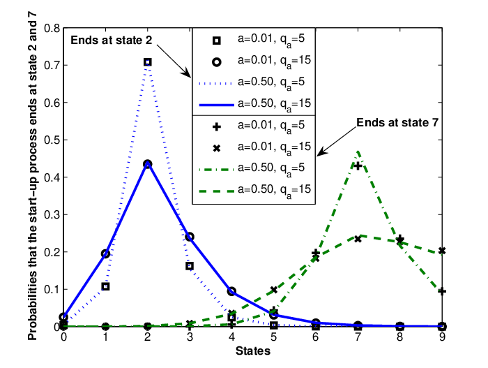
We first investigate how the playback variance influences the prefetching and the playback processes. Fig.11 shows the starvation probabilities when the start-up threshold and the variance change. When , the starvation probabilities computed from the VBR model are the same as those computed from the CBR model. While they differ greatly with . For the case , the jittering of playback rate influences the starvation probability more with than with . Fig.11 compares the probabilities that the prefetching process ends at the state 2 and 7 respectively. From this set of experiment, we can see that even does not obviously influence the prefetching.
Fig.14 compares the numerical results of VBR streaming with the model for CBR streaming. In our simulation, the mean frame size is 14400 bits. According to [19], the video frame size roughly follows Erlang distribution. If the Erlang distribution is the sum of i.i.d. exponentially distributed r.v.s., the mean of these r.v.s. is . We consider two cases in this set of experiments, (i.e. exponential r.v.) and . The resulting variances are (i.e. ) for and (i.e. ) for . The simulation time is playback slots. From Fig.14, we are surprised to see that the Erlang distributions of video frames do not obviously influence the starvation probabilities. The analytical framework for CBR streaming is good enough to model the starvation behavior for VBR streaming.
VI Extension to Fast Fading
This section models the starvation behavior of CBR streaming when users experience fast channel fading. We compute the first two moments of bit arrival process and show how these parameters can be feed into our analytical framework.
Network description. Due to the change of radio condition (e.g. user mobility, or a car passing by the user), the signal strength is no longer a constant at different scheduling slots. To explore the multiuser diversity gain, the base station adopts the normalized SNR scheduling algorithm for allocating time slots to coexisting flows.
We begin with the scenario with a fixed population of users (or flows) served by a single base station. In each slot, the users measure their channel qualities and feedback them to the BS. Based on the channel quality indications, the BS transmits to only one of the users every slot. Denote by the instantaneous signal to noise ratio (SNR) of user , (), at slot . As stated in most of previous work, we assume that all the users experience Rayleigh fast-fading. Denote by the average SNR of user . Then, the received SNR of user is an exponentially distributed random variable with the following probability density function The NSNR scheduler selects the user that has the highest relative SNR for transmission, where is the scheduled user at slot . In this section, we consider the case of homogeneous average SNRs (i.e. for all ). Therefore, the NSNR scheduler is equivalent to the maximum sum rate (MSR) scheduler that gives the largest per-user throughput.Since the SNRs of different users are independently distributed, the scheduled SNR, denoted by , has the following probability density function [24] Denote by the data rate of a user with the SNR . Here, can be a linear function in the low-SNR regime and a logarithmic function in the high SNR regime if the modulation scheme is continuous. For discrete modulations, is a step function of . Without loss of generality, we let .
Analysis of throughput process. The fast fading along with NSNR scheduling brings variation of bit arrivals to the receiver. The analytical framework for VBR streaming can be naturally extended to this scenario. The only modification lies in that the jittering of playback rate is substituted by that of bit arrivals. Therefore, we need the knowledge of the mean throughput and its variance measured in the duration of video contents. To achieve this goal, we must obtain the mean throughput and its variance measured in bits first.
Denote by the transmission rate of the user with the best SNR at a slot in each Hz when there are active flows in the cell. Denote by the transmission rate to one particular flow at a slot per Hz. Given the assumption that all the flows have the same average SNR, each flow has the equal probability of being scheduled. Hence, we can see
| (63) |
For the r.v. , its mean and variance are computed by
| (64) |
| (65) |
| (66) | |||||
| (67) | |||||
Denote by the duration of scheduling slot (usually 2ms), and by the width of wireless spectrum in Hz. Then, the mean and the variance of per-flow throughput measured in the duration of video contents are and respectively in one slot.
Let be the r.v. of per-flow throughput in one second that is measured by the duration of video contents. In one second, the total throughput of a flow at one Hz is the sum of throughput in slots. Therefore, the r.v. is the sum of i.i.d. r.v.s corresponding to the per-slot throughput. We can express the mean and the variance of as follows:
| (68) | |||||
| (69) | |||||
In general, the frequency width is 15 MHz, the bit-rate is usually greater than 200 Kbps, and equals to 0.002s. Then, is usually at the order of . If starvation happens at state , is usually less than 1, which means that needs to be small. However, the small results in the small variance . This is to say, if the variance of bit arrival process is large, there might not exist starvations. On the contrary, if the starvations appear, the variance is usually small so that its impact on the starvation is negligible. For this reason, we directly use the framework without diffusion approximation to model the streaming QoE in a fast fading channel.
Markov model of flow dynamics To analyze the interaction between NSNR scheduling and the flow dynamics, a fluid-level capacity model is required. When the average SNR of all active users are the same, the per-flow throughput in each slot is i.i.d. and only depends on the quantity of flows (see eq.(64)). Given the exponentially distributed video size, we can model the flow dynamics as a Markov process.
The Markov processes in Fig.2-4 contain transitions rates such as and . However, it is not direct to feed the parameters of this section into the above Markov processes. In Fig.2, state refers to the number of flows in the system. The departure rate is computed by for , recalling that is average per-user throughput in video duration per second. It is easy to obtain the stationary distribution of having flows by
(with the convention that over an empty set is 1). When a tagged user joins in the system and is also admitted, it observes other flows with the following stationary distribution
The Markov processes shown in Fig.3-4 are conditioned on the existence of the tagged flow. At state , the per-user throughput is because there are flows plus the tagged one. Hence, the transition rate is computed by for all . The transition rate is expressed as . Define as the total departure rate at state that has
| (70) |
in the presence of the tagged flow. The constants and are obtained by
| (71) |
Substituting the above parameters to the framework in section III, we can derive the approximated QoE metrics in a fast fading channel with flow dynamics.
Numerical Examples. Consider a wireless channel with frequency width of 1MHz. The average SNRs of users is 5dB. The base station allows at most 10 flows simultaneously, and schedules the transmission to one of them in every slot of duration 0.002s. The video duration is exponentially distributed with the mean of 90 seconds and the video bit rate is chosen to be 480Kbps. Then, the mean throughput are 3.5749, 2.3702, 1.7844, 1.4369, 1.2061, 1.0412, 0.9174, 0.8207, 0.7432, 0.6794 times the playback rate at states from 0 to 9. In other words, the mean throughput at states 69 are insufficient to support the continuous playback. The variances at all states are 0.0083, 0.0144, 0.0144, 0.0134, 0.0124, 0.0114, 0.0105, 0.0098, 0.0091, 0.0086, which are small enough. We consider two flow arrival rates, and . For , the traffic load is greater than 1 at states 05 and less than 1 at states 69. For the latter case, there have at all the states. Each set of simulation lasts time slots.
In Fig.14 we compare the starvation probabilities measured from a Rayleigh fading channel, and those computed from the model without considering throughput variation. The simulation matches the model quite well, which means that the flow-level dynamics have a dominant impact on the playback interruption, while the impact of throughput variation due to Rayleigh fading is negligible. In Fig.14 we examine the starvation probabilities when the playback process begins at different states. We test two start-up thresholds, , and two flow arrival rates, . One can observe that the starvation probabilities do not differ much in high states (e.g. 8 and 9). However, the starvation probabilities in the states with mean throughput around 1 are distinguishable, in which state 6 is an example. With , a tagged flow sees the congested network (more other flows) with a higher probability, and also encounters a higher probability of starvation afterwards.
VII Conclusions and Further Extensions
In this work, we developed an analytical framework to compute the QoE metrics of media streaming service in wireless data networks. Our framework takes into account the dynamics of playout buffer at three time scales, the scheduling duration, the video playback variation, as well as the flow arrivals or departures. We show that the proposed models can accurately predict the distribution of prefetching delay and the probability generating function of buffer starvations. The analytical results demonstrate that the flow dynamics have dominant influence on QoE metrics compared to the jittering in the throughput and the video playback rate.
Further Extensions: Our analytical framework can be adapted to the following scenarios: i) hyper-exponential video length distribution, ii) heterogeneous channel gains, and iii) mixed data and streaming flows. The heterogeneity of video durations, channel gains, and traffic types requires the classification of flows. The heterogeneous video duration is usually modeled by the hyper-exponential distribution. Users requesting the videos of the same exponential distribution fall in one class. The same argument holds in the case of heterogeneous SNRs among users. We can group the users with more or less the same average SNR in the same class (e.g. see [25]). The service times are still exponentially distributed, but with different parameters in different user classes. When classes are introduced, the Markov process are thus modified to contain multi-dimensional states, representing the number of (observed) flows in different classes. We can then construct the PDEs and the ODEs on top of them.
References
- [1] Allot MobileTrends. http://www.allot.com.
- [2] S. Borst and N. Hegde, “Integration of Streaming and Elastic Traffic in Wireless Networks”, Infocom 2007.
- [3] K. Stuhlmuller et al, “Analysis of video transmission over lossy channels”, IEEE JSAC, 2000.
- [4] R. Zhang, S. L. Regunathan, and K. Rose, “Video coding with optimal inter/intra-mode switching for packet loss resilience”, IEEE J. Sel. Areas Commun., 2000.
- [5] Z.H. He, et al, “Joint Source Channel Rate-Distortion Analysis for Adaptive Mode Selection and Rate Control in Wireless Video Coding”, IEEE JSAC 12(6)):511-523, 2002
- [6] L. Rong, S-E. Elayoubi and O. Ben Haddada, “Performance Evaluation of Cellular Networks Offering TV Services”, IEEE Transa. on Vehicular Tech., 2010.
- [7] M. K. Karray, “Analytical evaluation of QoS in the downlink of OFDMA wireless cellular networks serving streaming and elastic traffic” IEEE Trans. on Wireless Commun., 2010.
- [8] Y.D. Xu, E. Altman, et. al, “Probabilistic Analysis of Buffer Starvation in Markovian Queues”, IEEE Infocom 2012.
- [9] Y.D. Xu, E. Altman, et. al, “QoE Analysis of Media Streaming in Wireless Data Networks”, IFIP Networking 2012.
- [10] Hao Luan, Lin X. Cai, and Xuemin (Sherman) Shen, “Impact of network dynamics on users’ video quality: analytical framework and QoS provision” IEEE Trans. on Multimedia, Vol.12, No.1, pp:64-78, 2010.
- [11] G. Liang and B. Liang, “Effect of delay and buffering on jitter-free streaming over random VBR channels”, IEEE Trans. on Multimedia, Vol.10, No.6 pp:1128-1141, 2008.
- [12] A. ParandehGheibi et al, “Avoiding Interruptions a QoE Reliability Function for Streaming Media Applications”, IEEE J. Sel. Areas Commun., Vol.29, No.5, pp:1064-1074, 2011.
- [13] H. Sanneck, G. Carle, and R. Koodli, “ A framework model for packet loss metrics based on loss run length,” Proc. of ACM SIGMM 2000.
- [14] L. Takacs, “Ballot problems”, Prob. Theory Related Fields, Vol. 1, No.2, pp:154-158, 1962.
- [15] T. Bonald and A. Proutiere, “A Queueing Analysis of Data Networks”, Queueing Networks, Springer, 2011.
- [16] J.G. Choi and S. Bahk, “Cell-throughput analysis of the proportional fair scheduler in the single-cell environment,” IEEE Trans. Veh. Technol., Vol, 56, pp:766-778, 2007.
- [17] G. Song and Y. Li, “Asymptotic throughput analysis for channel-aware scheduling,” IEEE Trans. Commun., Vol.54, No.10, pp.1827-1834, 2006.
- [18] H.J. Kushner and P.A. Whiting, “Convergence of proportional-fair sharing algorithms under general conditions”, IEEE Trans. Wireless Commun., Vol.3, No.4, pp.1250-1259, 2004.
- [19] D. Masi, M. Fischer, D. Garbin, “Video Frame Size Distribution Analysis,” The Telecom. Rev., 19, 2008.
- [20] F. Dobrian, A. Awan, I. Stoica, et.al, “Understanding the Impact of Video Quality on User Engagement”, ACM SIGCOMM’2011.
- [21] S. Elayoubi and B. Fourestie, “Performance evaluation of admission control and adaptive modulation in OFDMA WiMax systems”, IEEE/ACM Trans. Networking, 16(5), 2008.
- [22] Y. Lu and C.L. Tsai, “The expected discounted penalty at ruin for a Markov-Modulated risk process perturbed by diffusion,” North Amer. Actuarial J. 11(2):136-152, 2008.
- [23] F. Dufresne, H.U. Gerber, “Risk theory for the compound Poisson process that is perturbed by diffusion”, Insurance: Mathematics and Economics, Vol.10, pp:51-59, 1991.
- [24] Y.J. Chang, F.T. Chien, and C.C. Kuo, “Cross-layer QoS Analysis of Opportunistic OFDM-TDMA and OFDMA Networks”, IEEE J. Sel. Areas Commun., Vol.25, 2007.
- [25] S. Borst, “User-Level Performance of Channel-Aware Scheduling Algorithms in Wireless Data Networks”, Proc. of IEEE Infocom 2003.
- [26] B. Wang, W. Wei, Z. Guo and D. Towsley, “Multimedia Streaming via TCP: An Analytic Performance Study”, ACM TOMCCAP, Vol.5, No.3, pp:1-23, 2004.
- [27] G.A. Geist, “Reduction of a general matrix to tridiagonal form”, SIAM. J. Matrix Anal. & Appl., Vol.12, No.2, pp:362-373, 1991.
- [28] G.H. Golub, and V.F. Van Loan, Matrix Computations, John Hopkins University Press, 3rd, pp:439-445, 1996.
- [29] X. Cheng, C. Dale, and J.C. Liu “Statistics and social networks of Youtube videos”, Proc. of IEEE IWQoS., pp:229-238, 2008.
- [30] F. Czachorski, “Diffusion approximation as a modelling tool in congestion control and performance evaluation”, Proc. of HET-NET., 2004.
Appendix
VII-A Solving PDEs
Suppose that is a function of variable where and are expressed as and . We take first-order derivative of over and obtain
| (72) |
We first solve the following homogeneous PDEs originated from Eq.(12)
| (73) |
Comparing Eqs.(72) with Eqs.(73), we have
| (74) |
The above simple differential equations give rise to
In general, is set to 0 such that there have
Then, is a function of the variable . Define to be a continuous and differentiable function in the range . is solved by
| (75) |
when the PDEs are homogeneous. We next proceed to consider the inhomogeneous parts at Eqs.(12) in the matrix form
| (76) |
Then, there has
| (77) | |||||
where denotes a column vector of for all . Due to the discontinuity of at the point , we propose to solve it using the known results in Brownian motion. The arrival rate of streaming packets at state is , measured in seconds. We add a very small variance to the arrival rate where the standard deviation is denoted by . We use Brownian motion to approximate the arrival rate of streaming packets. According to [10, 30], the solutions of the homogeneous PDEs are approximated by
| (78) |
given is small enough. Submitting Eq.(78) to Eq.(77), we solve the inhomegeneous PDEs by
| (79) | |||||
VII-B Proof of Lemma 1
Proof: Without loss of generality, we consider a tridiagonal matrix in the form
where are all real constants. Our claim is a natural conclusion of the following lemma.
Lemma 2
[27] Assume that the coefficients , are nonzero, and the products are positive. Then, the matrix is similar to a symmetric tridiagonal matrix. Therefore, its eigenvalues are all real.
Here, satisfies the conditions in the above lemma. Thus, is similar to a symmetric matrix, and is diagonizable. According to Gershgorin circle theorem [28], every eigenvalue of lies within at least one of the Gershgorin discs. Because the diagonal element is positive, and is larger than the sum of absolution values of non-diagonal elements in each line, every eigenvalue cannot be negative. This concludes the proof.